| Issue |
A&A
Volume 521, October 2010
|
|
|---|---|---|
| Article Number | A3 | |
| Number of page(s) | 12 | |
| Section | Interstellar and circumstellar matter | |
| DOI | https://doi.org/10.1051/0004-6361/201014911 | |
| Published online | 13 October 2010 | |
The population of planetary nebulae and H II regions in M 81
A study of radial metallicity gradients and chemical evolution![[*]](/icons/foot_motif.png)
L. Stanghellini1 - L. Magrini2 - E. Villaver3 - D. Galli2
1 -
National Optical Astronomy Observatories, Tucson, AZ 85719, USA
2 -
INAF-Osservatorio Astrofisico di Arcetri, Largo E. Fermi 5, 50125 Firenze, Italy
3 -
Universidad Autónoma de Madrid, Departamento de Física Teórica C-XI, 28049 Madrid, Spain
Received 1 May 2010 / Accepted 14 June 2010
Abstract
Context. M 81 is an ideal laboratory to investigate the
galactic chemical and dynamical evolution through the study of its
young and old stellar populations.
Aims. We analyze the chemical abundances of planetary nebulae and H II regions
in the M 81 disk for insight on galactic evolution, and compare it
with that of other galaxies, including the Milky Way.
Methods. We acquired Hectospec/MMT spectra of 39 PNe and 20 H II
regions, with 33 spectra viable for temperature and abundance analysis.
Our PN observations represent the first PN spectra in M 81 ever
published, while several H II region spectra have
been published before, although without a direct electron temperature
determination. We determine elemental abundances of helium, nitrogen,
oxygen, neon, sulfur, and argon in PNe and H II regions, and determine their averages and radial gradients.
Results. The average O/H ratio of PNe compared to that of the H II regions indicates a general oxygen enrichment in M 81 in the last ![]() 10 Gyr. The PN metallicity gradient in the disk of M 81 is
10 Gyr. The PN metallicity gradient in the disk of M 81 is
![]() dex/kpc.
Neon and sulfur in PNe have a radial distribution similar to that of
oxygen, with similar gradient slopes. If we combine our H II
sample with the one in the literature we find a possible mild evolution
of the gradient slope, with results consistent with gradient steepening
with time. Additional spectroscopy is needed to confirm this trend.
There are no type I PNe in our M 81 sample, consistently with
the observation of only the brightest bins of the PNLF, the galaxy
metallicity, and the evolution of post-AGB shells.
dex/kpc.
Neon and sulfur in PNe have a radial distribution similar to that of
oxygen, with similar gradient slopes. If we combine our H II
sample with the one in the literature we find a possible mild evolution
of the gradient slope, with results consistent with gradient steepening
with time. Additional spectroscopy is needed to confirm this trend.
There are no type I PNe in our M 81 sample, consistently with
the observation of only the brightest bins of the PNLF, the galaxy
metallicity, and the evolution of post-AGB shells.
Conclusions. Both the young and the old populations of M 81
disclose shallow but detectable negative radial metallicity gradient,
which could be slightly steeper for the young population, thus not
excluding a mild gradients steepening with the time since galaxy
formation. During its evolution M 81 has been producing oxygen;
its total oxygen enrichment exceeds that of other nearby galaxies.
Key words: ISM: abundances - H II regions - planetary nebulae: general - galaxies: abundances - galaxies: evolution - galaxies: clusters: individual: M 81
1 Introduction
The study of chemical evolution of galaxies hinges on the confrontation between sets of evolutionary chemical models and arrays of observational data. Comparison of models with reliable abundance determinations are needed to understand the framework of galaxy evolution, and to test star formation history, stellar nucleosynthesis, and the mechanisms of galaxy assembly and formation.
Galactic metallicity gradients, and especially their time evolution, are important probes of galaxy formation and evolution. Observationally, most studied galaxies display a radial metallicity gradient with a negative slope, indicative of higher metallicity toward the inner galaxy. Time variation of gradient slopes in galaxies is hard to come by, given the lack of reliable time-tagging metallicity probes. From the viewpoint of theory, different models predict opposite time evolution of the metallicity gradient, showing the sensitivity of this physical parameter to the adopted parameterization of the processes (e.g., Magrini et al. 2007). A key factor to forwarding our knowledge in this field is the acquisition of high quality spectra to obtain abundances for a variety of probes, in a wide selection of different galaxies, including our own, to cover as much as possible the parameter space of initial masses, metallicities, and galaxy type.
The planetary nebula (PN) abundances of elements that are invariant during the evolution of low-
and intermediate-mass stars (the so-called ![]() -elements)
probe the environment at the epoch of the formation of the PN
progenitors. Oxygen, neon, sulfur, and argon are, for the most part,
manufactured in high mass stars (
-elements)
probe the environment at the epoch of the formation of the PN
progenitors. Oxygen, neon, sulfur, and argon are, for the most part,
manufactured in high mass stars (
![]() ), thus their concentration in PNe across galactic
disks probe the metallicity gradient in remote epochs. The metallicity gradients of PNe, compared
to gradients of young stellar populations (such as those given by H II regions) allow the study of
the chemical evolution of galaxies. Galactic metallicity gradients are measured in terms of
), thus their concentration in PNe across galactic
disks probe the metallicity gradient in remote epochs. The metallicity gradients of PNe, compared
to gradients of young stellar populations (such as those given by H II regions) allow the study of
the chemical evolution of galaxies. Galactic metallicity gradients are measured in terms of
![]() log (X/H)/
log (X/H)/
![]() dex kpc-1, where X/H is the abundance of element X with respect to hydrogen and
dex kpc-1, where X/H is the abundance of element X with respect to hydrogen and ![]() is the galactocentric distance.
is the galactocentric distance.
Planetary nebula gradients in the Milky Way indicate that the
metallicity decreases inside out by 0.01 to 0.07 dex kpc-1 (e.g., Maciel & Quireza 1999; Henry et al. 2004; Stanghellini et al. 2006; Perinotto & Morbidelli 2006).
The most recent of these studies seem to agree that the PN metallicity
gradients are rather flat, i.e., their slope is not steeper than ![]() -0.02 dex kpc-1, and only slightly shallower than that derived from H II regions,
implying that the Galactic metallicity gradient does not vary very much
within the time frame of Galactic evolution. The metallicity gradients
based on Galactic PNe are hindered by the uncertainties in PN
distances, by the interstellar absorption in the direction of the
Galactic center, and by the paucity of PN observations in the direction
of the Galactic anti-center. These factors, together with the interest
of studying metallicity gradients of other spiral galaxies of different
morphological types and belonging to different groups, prompt us to
investigate the PN (and H II region) metallicity gradients in the M 81 disk.
-0.02 dex kpc-1, and only slightly shallower than that derived from H II regions,
implying that the Galactic metallicity gradient does not vary very much
within the time frame of Galactic evolution. The metallicity gradients
based on Galactic PNe are hindered by the uncertainties in PN
distances, by the interstellar absorption in the direction of the
Galactic center, and by the paucity of PN observations in the direction
of the Galactic anti-center. These factors, together with the interest
of studying metallicity gradients of other spiral galaxies of different
morphological types and belonging to different groups, prompt us to
investigate the PN (and H II region) metallicity gradients in the M 81 disk.
M 81 is the largest member of the nearest interacting group of galaxies at a distance of
![]() Mpc (Freedman et al. 2001).
Its two brightest companions, M 82 and NGC 3077, are located
within a projected distance of 60 kpc. The disturbed nature of the
system is evident from the observations in the 21 cm emission line
of H I, showing extended tidal streams and debris between the galaxies (Gottesman & Weliachew 1975; Yun et al. 1994). The simulation of Yun (1999) explains many of these tidal features as being the result of close encounters between M 81
and each of its neighbors
Mpc (Freedman et al. 2001).
Its two brightest companions, M 82 and NGC 3077, are located
within a projected distance of 60 kpc. The disturbed nature of the
system is evident from the observations in the 21 cm emission line
of H I, showing extended tidal streams and debris between the galaxies (Gottesman & Weliachew 1975; Yun et al. 1994). The simulation of Yun (1999) explains many of these tidal features as being the result of close encounters between M 81
and each of its neighbors ![]() 200-300 Myr ago. The most prominent debris
(e.g., Sabbi et al. 2008; Weisz et al. 2008) are considered tidal dwarf galaxies,
new stellar systems that formed in gas stripped from interacting galaxies.
200-300 Myr ago. The most prominent debris
(e.g., Sabbi et al. 2008; Weisz et al. 2008) are considered tidal dwarf galaxies,
new stellar systems that formed in gas stripped from interacting galaxies.
The ![]() -element abundances of PNe and H II regions in M 81 have remained elusive, with the exception of 17 H II regions (Garnett & Shields 1987, GS87). With the PNe (Jacoby et al. 1989; Magrini et al. 2001) and H II regions (Lin et al. 2003) locations, and their de-projected (PA = 157
-element abundances of PNe and H II regions in M 81 have remained elusive, with the exception of 17 H II regions (Garnett & Shields 1987, GS87). With the PNe (Jacoby et al. 1989; Magrini et al. 2001) and H II regions (Lin et al. 2003) locations, and their de-projected (PA = 157![]() and inclination = 59
and inclination = 59![]() ,
Kong et al. 2000)
galactocentric distances available we are in the position to push
forward a determination of abundance gradients from PNe and H II regions
in the M 81 disk. The location of M 81 within its group will
allow us to study the effect of galaxy interactions and mergers in the
evolution of a galaxy and of its abundance gradient.
,
Kong et al. 2000)
galactocentric distances available we are in the position to push
forward a determination of abundance gradients from PNe and H II regions
in the M 81 disk. The location of M 81 within its group will
allow us to study the effect of galaxy interactions and mergers in the
evolution of a galaxy and of its abundance gradient.
In order to sample the M 81 disk to the necessary S/N for abundance analysis we need spectroscopy with a 6-8 m class telescope. MMT/Hectospec medium-resolution spectroscopy offers the unique opportunity to study both the PNe and the H II region populations with the same setup, during the same night, and adopting the same analysis techniques, thus avoiding most biases that commonly affect the comparison of chemical abundances in population of different ages (e.g. Fe/H from old RGB stars is difficult to compare with O/H from the present time H II regions). We present here the results from the study of a sample of bright PNe in M 81, with the goal of obtaining the metallicity and explore their gradients within the M 81 disk. Their properties as a group are discussed, and compared with those of H II regions from both our MMT observations and from the literature. The combined properties of M 81 PNe and H II regions are also compared with their homologs in other nearby galaxies and in the Milky Way.
In Sect. 2 we describe the observation and analysis techniques, and give the measured fluxes and calculated abundances. Section 3 includes the analysis of the derived abundances and the determination of the metallicity gradients, Sect. 4 presents the discussion of our results, and the conclusions are in Sect. 5.
2 The MMT observations: data reduction and analysis
2.1 Observations
We obtained the spectra of PNe and H II regions in M 81 with the MMT Hectospec fiber-fed spectrograph (Fabricant et al. 2005). The spectrograph was equipped with an Atmospheric Dispersion Corrector and it was used with a single setup: 270 mm-1 grating at a dispersion of 1.2 Å pixel-1. The resulting total spectral coverage ranged from approximately 3600 Å to 9100 Å, thus including the basic emission-lines necessary for the determination of physical and chemical properties.
The PNe were selected among those observed with the Isaac Newton Telescope (INT) with [O III], H![]() ,
and Stromgren Y
filters (Magrini et al. 2001), which allowed us to cover the whole
field of M 81, and to identify a large number of disk PNe at large galactocentric distances.
An earlier survey by Jacoby et al. (1989) was limited to the M 81 bulge.
It is worth noting that the INT images allow us to have accurate positions (<0.5
,
and Stromgren Y
filters (Magrini et al. 2001), which allowed us to cover the whole
field of M 81, and to identify a large number of disk PNe at large galactocentric distances.
An earlier survey by Jacoby et al. (1989) was limited to the M 81 bulge.
It is worth noting that the INT images allow us to have accurate positions (<0.5
![]() )
and
finding charts for the selected PNe and H II regions, a crucial information given the crowding of
the inner and spiral arm fields of M 81.
)
and
finding charts for the selected PNe and H II regions, a crucial information given the crowding of
the inner and spiral arm fields of M 81.
The first target selection was performed by scaling the PN brightness in [O III]
with
those of M 33 PNe, whose medium-resolution spectra have been
observed by us using the identical technique (Magrini et al. 2009, 2010, hereafter M09, M10).
We also endeavored to have PN targets at several galactocentric distances, in order to characterize
the PN metallicity gradient. The instrument deploys 300 fibers
over a 1 degree diameter field of view and the fiber diameter is ![]() 1.5
1.5
![]() .
The projected size of M 81 on the sky is smaller than the whole
field of view of MTT/Hectospec, and we took advantage of this by placing some of
the fibers in the outermost periphery of M 81, where some H II regions and few PNe, both belonging to the outer disk and to the intra-group population, have been identified.
In addition, since the available catalog of H II regions by Lin et al. (2003) is based on H
.
The projected size of M 81 on the sky is smaller than the whole
field of view of MTT/Hectospec, and we took advantage of this by placing some of
the fibers in the outermost periphery of M 81, where some H II regions and few PNe, both belonging to the outer disk and to the intra-group population, have been identified.
In addition, since the available catalog of H II regions by Lin et al. (2003) is based on H![]() photometry, our INT [O III] observations have been useful to select [O III]-bright H II regions essential for chemical abundance determination. As stated by Magrini et al. (2001), we expect the misclassification of H II regions into PNe and vice-versa to be lower than
photometry, our INT [O III] observations have been useful to select [O III]-bright H II regions essential for chemical abundance determination. As stated by Magrini et al. (2001), we expect the misclassification of H II regions into PNe and vice-versa to be lower than ![]() 3
3![]() of the whole sample.
of the whole sample.
The observations were carried out in queue mode in four runs during the months of November and December 2008. Each of the observing runs consisted of 3 to 5 exposures of 1800 s each, for a total of 16 exposures (or 8 h of observation). We used the same fiber setup during all observing runs, and thus PNe and H II regions were observed within the same conditions, including the same exposure time. Priority was given to PNe when placing the fibers, since a set of H II region spectra already exists in the literature (GS87). A large number of fibers were devoted to sky measurements, to ensure that sky spectra were obtained in several positions around each target.
Cosmic rays were removed with the appropriate hectospec.hcosmic routine in the hectospec analysis package. Cosmic rays are detected via subtraction of multiple images, flagging the high or low pixels. The flagged pixels are interpolated over, and the resultant images are combined by average. This method avoids problems with clipping that other programs suffer from. In order to perform the sky subtraction we first inspected the sky spectra and eliminated those with unusual signals. Then we averaged the six spectra closer (in fiber location) to the targets, scaled the result to match the object spectrum, and subtracted.
The spectral calibration was achieved with the standard star Hilt600 (Massey et al. 1988), observed during the first night. This star was chosen by its excellent spectral coverage compared to the spectra of the PNe. It is worth noting that our analysis does not hinge on flux calibration, rather spectral calibration and flux ratios, thus this approach is sufficient to the science goals. Other stars were observed during the run nights, but the excellent spectral coverage of Hilt600 makes it the ideal choice for this type of calibration. Variations in sky conditions are taken into account since sky subtraction was performed before flux calibration.
In Table 1 we give the IDs, equatorial coordinates, and equivalent [O III] magnitude of the planetary nebulae and H II regions observed with MMT medium-resolution spectroscopy. All PN IDs are from Magrini et al. (2001), except for PN4 and PN5, which are identified PNe with unpublished positions (Magrini, private communication). There are 39 PNe and 20 H II regions whose spectra have been acquired and analyzed. With the exception of PN 49m and PN 79m, whose spectral lines are below the detection limit, we detect at least the major spectral lines in each target.
Table 1: Observing log.
In Table 2, available
online in its completeness, we give for each target the ion and
wavelength (Cols. 1 and 2) of the observed emission line,
then the relative observed flux
(Col. 3), its uncertainty (Col. 4), and the line intensity
(Col. 5) obtained with the extinction correction given as a header
for each target. All fluxes and intensities are normalized for
![]() and
and
![]() .
Both PNe and H II regions are listed in Table 2.
Target names are given for each target at the head of the corresponding flux list.
The emission-line fluxes were measured with the package SPLOT of IRAF
.
Both PNe and H II regions are listed in Table 2.
Target names are given for each target at the head of the corresponding flux list.
The emission-line fluxes were measured with the package SPLOT of IRAF![]() . Errors in the fluxes
were calculated taking into account the statistical error in the
measurement of the fluxes, as well as systematic errors of the flux
calibrations, background determination, and sky subtraction. Observations of same
objects during different runs were stacked together and the resulting spectra have
been used for the analysis.
. Errors in the fluxes
were calculated taking into account the statistical error in the
measurement of the fluxes, as well as systematic errors of the flux
calibrations, background determination, and sky subtraction. Observations of same
objects during different runs were stacked together and the resulting spectra have
been used for the analysis.
![\begin{figure}
\par\includegraphics[width=16.5cm,clip]{14911fg1-NEW.eps}
\end{figure}](/articles/aa/full_html/2010/13/aa14911-10/img19.png)
|
Figure 1: Sample of medium-resolution spectra of M 81 PNe. |
| Open with DEXTER | |
We derived c(H![]() ) from the H
) from the H![]() /H
/H![]() flux ratios, as described in M09, and used the Galactic extinction curve by Mathis (1990) to correct the observed flux for interstellar extinction.
In a few PNe the derived intensity of the H
flux ratios, as described in M09, and used the Galactic extinction curve by Mathis (1990) to correct the observed flux for interstellar extinction.
In a few PNe the derived intensity of the H![]() line is more than 30
line is more than 30![]() off the theoretical prediction (
I4340=0.466 for
off the theoretical prediction (
I4340=0.466 for
![]() K, case B, Oserbrock & Ferland 2006).
The reason for this offset could be an uncertain c(H
K, case B, Oserbrock & Ferland 2006).
The reason for this offset could be an uncertain c(H![]() ). The average c(H
). The average c(H![]() )
calculated for our PNe is
)
calculated for our PNe is
![]() ,
a reasonable value if we consider the average c(H
,
a reasonable value if we consider the average c(H![]() )
of Galactic PNe (from Cahn et al. 1992,
)
of Galactic PNe (from Cahn et al. 1992, ![]() c(H
c(H![]() )
)
![]() )
and the relative metallicities of the Galaxy to M 81. We will
recall these outliers later in the discussion and indicate them with
different symbols in the figures.
)
and the relative metallicities of the Galaxy to M 81. We will
recall these outliers later in the discussion and indicate them with
different symbols in the figures.
To our knowledge, this is the first attempt in the literature to detect PN emission line fluxes in M 81 thus we cannot extend our discussion to comparison with previous work. The spectral quality is excellent. In Fig. 1 we show a few examples of our M 81 PN spectra, where the plasma and abundance diagnostic lines are well evident, and the S/N obtained with our observations makes us confident on the data quality.
Several H II regions have been already observed by GS87, where the Authors refer to the catalog by Hodge & Kennicutt (1983) for coordinates. Since the latter are given in image coordinates rather than Galactic coordinates, it has been hard to eliminate from our sample of H II regions those that have been already analyzed by GS87 or comparing targets from the two sets. But by comparing the position visually, we did not find any obvious overlap between the two samples, thus cannot compare the results.
2.2 Plasma diagnostics
We perform plasma diagnostics by using the 5-level atom model included in the nebular
analysis package in IRAF/STSDAS (Shaw & Dufour 1994), consistently with our work in M 33 (M09, M10). To calculate densities we use the doublet of the sulfur lines
[S II]
![]() 6716, 6731, while for the electron temperatures we
use the ratios [O III]
6716, 6731, while for the electron temperatures we
use the ratios [O III]![]() 4363/(
4363/(![]() 5007 +
5007 + ![]() 4959), [N II]
4959), [N II]![]() 5755/(
5755/(![]() 6548 +
6548 + ![]() 6584), and [S III]
6584), and [S III]![]() 6312/(
6312/(![]() 9059 +
9059 + ![]() 9532). In some cases, even if the sulfur lines are available,
their ratio is outside the diagnostic ranges for density calculation (e.g., Stanghellini & Kaler 1989), and we assumed a density of 103 cm-3.
We calculate the medium- and low-excitation temperatures
respectively from the [O III] and [S III], and from the [N II] line ratios, respectively (see also
Osterbrock & Ferland 2006, Sect. 5.2).
9532). In some cases, even if the sulfur lines are available,
their ratio is outside the diagnostic ranges for density calculation (e.g., Stanghellini & Kaler 1989), and we assumed a density of 103 cm-3.
We calculate the medium- and low-excitation temperatures
respectively from the [O III] and [S III], and from the [N II] line ratios, respectively (see also
Osterbrock & Ferland 2006, Sect. 5.2).
Table 2: Observed fluxes and line intensities.
2.3 Abundance analysis
Of the 39 PNe with emission line spectra, [O III] and [N II] temperature diagnostics are available respectively for 10 and 12 PNe, with only 3 PNe in common. In the analysis of the M 33 PNe (M09) we were able to infer the electron temperature for targets whose plasma diagnostics were not available by using the correlation between the electron temperature and the He II line intensity. In the case of M 81 none of the PNe show the He II emission; as a consequence, abundance analysis was possible only for the 19 PNe where electron temperature was diagnosed directly. There are also 14 H II regions whose temperature analysis was based on auroral lines, and their plasma and abundance analysis was performed in a similar way than for the PNe. Electron temperature diagnostics for more than one excitation state was available for 5 of the 14 regions.
The plasma diagnostics are given in Table 3, available online, together with the ionic abundances of the PNe and H II regions. Column (1) gives the diagnostics, and Col. (2) the value as determined from our analysis. The targets are listed sequentially, as in Table 1, and the first line for each target gives the target name.
Table 3: Plasma analysis and abundances.
The abundance analysis of the PNe and the H II regions was performed following the prescription given by M09, M10; abundances of all elements except helium where
calculated with the ionization correction factors (ICFs) given in Kingsburgh & Barlow (1994) for the case were only optical lines are detected. Where both ![]() [O III] and
[O III] and ![]() [N II] were available we used
[N II] were available we used ![]() [O III] to derive the abundances of medium and high excitation
ions, and
[O III] to derive the abundances of medium and high excitation
ions, and ![]() [N II] for the low excitation ones. In several H II
regions the temperature from the auroral line of [SIII] were also
available, corresponding to transition of intermediate excitation. If
only one of the electron temperature diagnostics was available we use
that temperature to derive abundances for all ions. Helium abundances
were calculated with the formulation of Benjamin et al. (1999) in two density regimes, and taking into account Clegg's (1987) collisional populations, as in M09.
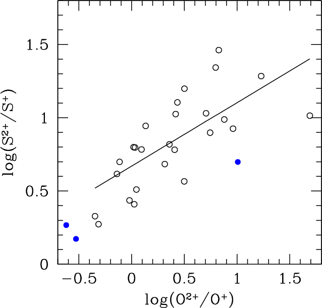
The sulfur abundances for our PNe are mostly based on [S II] lines, thus highly unreliable. We used the interpolation to the Galactic PN data by Kingsburgh & Barlow to infer [S III]/[S II] from the [O III]/[O II] ratios, where possible, and obtained an estimate of [S III], which is observed only in three PNe. In order to check whether the sulfur correction is sensible, in Fig. 2 we plot log
[N II] for the low excitation ones. In several H II
regions the temperature from the auroral line of [SIII] were also
available, corresponding to transition of intermediate excitation. If
only one of the electron temperature diagnostics was available we use
that temperature to derive abundances for all ions. Helium abundances
were calculated with the formulation of Benjamin et al. (1999) in two density regimes, and taking into account Clegg's (1987) collisional populations, as in M09.
The sulfur abundances for our PNe are mostly based on [S II] lines, thus highly unreliable. We used the interpolation to the Galactic PN data by Kingsburgh & Barlow to infer [S III]/[S II] from the [O III]/[O II] ratios, where possible, and obtained an estimate of [S III], which is observed only in three PNe. In order to check whether the sulfur correction is sensible, in Fig. 2 we plot log
![]() versus log
versus log
![]() for the Kingsburgh & Barlow
sample. On the same plot we locate our M 81 PNe with measured [S III].
The solid line, representing
for the Kingsburgh & Barlow
sample. On the same plot we locate our M 81 PNe with measured [S III].
The solid line, representing
![]() ,
has the correct slope for both the Galactic and M 81 data, but it overcorrect slightly for [S III]. Since the [S III] lines we observe in M 81 are quite faint, the
relation by Kingsburgh & Barlow (1994) seems reasonable.
,
has the correct slope for both the Galactic and M 81 data, but it overcorrect slightly for [S III]. Since the [S III] lines we observe in M 81 are quite faint, the
relation by Kingsburgh & Barlow (1994) seems reasonable.
|
Figure 2: The log(S2+/log(S+) versus log(O2+/log(O+) correlation (solid line), based on the Galactic PNe from Kingsburgh & Barlow (1994, open circles). Our targets are shown with filled circles. |
| Open with DEXTER | |
Table 4: Temperatures and abundances uncertainties.
Table 5: Galactocentric distances and elemental abundances.
The formal errors in the ionic and total abundances were
computed taking into account the uncertainties in (i) the observed
fluxes; (ii) the electron temperatures and densities; and (iii) c(H![]() ).
We performed complete formal error propagation for a subsample of
target, representing a spread of flux error and magnitudes, and
realized that the errors in the electron temperature
completely dominate the errors in the ionic abundances for all elements
except helium. In particular, the flux uncertainty of the weaker of the
diagnostic lines
in the electron temperatures,
).
We performed complete formal error propagation for a subsample of
target, representing a spread of flux error and magnitudes, and
realized that the errors in the electron temperature
completely dominate the errors in the ionic abundances for all elements
except helium. In particular, the flux uncertainty of the weaker of the
diagnostic lines
in the electron temperatures, ![]() 5755 for
5755 for ![]() [N II] and
[N II] and ![]() 4363 for
4363 for ![]() [O III], determine the errors in the abundances. In Table 4
we give the error analysis for the PN subsample, including the ones
with the minimum and maximum flux errors; Col. (1) gives the PN
name,
Col. (2) gives the relative flux error for the weaker line in the
temperature diagnostics (in PN 9m we could calculate both
[O III], determine the errors in the abundances. In Table 4
we give the error analysis for the PN subsample, including the ones
with the minimum and maximum flux errors; Col. (1) gives the PN
name,
Col. (2) gives the relative flux error for the weaker line in the
temperature diagnostics (in PN 9m we could calculate both ![]() [N II] and
[N II] and ![]() [O III], thus we give the two errors), Cols. (3) and (4) give the relative errors in
[O III], thus we give the two errors), Cols. (3) and (4) give the relative errors in ![]() [N II] and
[N II] and ![]() [O III] respectively, and finally Cols. (5) through (7)
give the abundance errors, in dex. We derived the errors for all other targets by interpolation of the
[O III] respectively, and finally Cols. (5) through (7)
give the abundance errors, in dex. We derived the errors for all other targets by interpolation of the
![]() (X) curves. In the case of the helium abundances we run the error analysis by using the formulae by Benjamin et al. (1999), and found that the factor determining the uncertainties is the relative error on the helium flux lines.
The abundances, their uncertainties, together with the galactocentric distances (see Sect. 3.1) are given in Table 5.
(X) curves. In the case of the helium abundances we run the error analysis by using the formulae by Benjamin et al. (1999), and found that the factor determining the uncertainties is the relative error on the helium flux lines.
The abundances, their uncertainties, together with the galactocentric distances (see Sect. 3.1) are given in Table 5.
It is worth noting that another source of error that we could not
estimate explicitly is intrinsic to the ICF method. The uncertainties
due to the ICF are very moderate for oxygen, but can be quite large for
the other atoms, especially sulfur, thus these abundance uncertainties
should be considered as formal errors, but might underestimate the real
uncertainties.
Another source of abundance uncertainties is the use of a single
electron temperature for both low- and high-ionization ions. This
regards the 16 PNe and 9 H II
regions where only one choice of the electron temperature was
available. We have analyzed the sample of targets where two electron
temperatures were available, and found that the average difference
between electron temperatures of the order of 20![]() .
We tested that the resulting atomic abundance uncertainties are lower than those due to flux errors on the auroral lines.
.
We tested that the resulting atomic abundance uncertainties are lower than those due to flux errors on the auroral lines.
The sets where we have oxygen and neon in common is limited to 6 PNe and 7 H II regions.
There is a clear correlation between these two ![]() -elements in both sets, with correlation coefficients
-elements in both sets, with correlation coefficients
![]() and 0.9 respectively for PNe and H II
regions. This high correlation is expected, since both elements are
produced in the type II SN environment. The large uncertainties in
the sulfur abundances make the comparison between oxygen and sulfur
less meaningful, although the two sets have higher overlap than the
previously described pair (16 PNe and 14 H II regions in common), the correlation coefficient is only 0.4 and 0.3 for the two sets.
and 0.9 respectively for PNe and H II
regions. This high correlation is expected, since both elements are
produced in the type II SN environment. The large uncertainties in
the sulfur abundances make the comparison between oxygen and sulfur
less meaningful, although the two sets have higher overlap than the
previously described pair (16 PNe and 14 H II regions in common), the correlation coefficient is only 0.4 and 0.3 for the two sets.
|
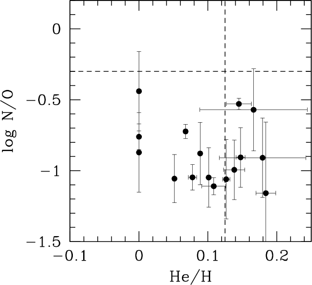
Figure 3: log (N/O) vs. He/H; broken lines show He/H = .125 and log(N/O) = -0.3. Type I PNe would be located in the upper-right quadrant. |
| Open with DEXTER | |
Figure 3 shows the log(N/O) vs. helium plot, to classify Type I PNe. These are the nitrogen and helium-enriched PNe, whose progenitors have likely undergo the third dredge-up and hot bottom-burning, and thus are likely to have higher progenitor masses (Peimbert & Torres-Peimbert 1983; Marigo 2001). The top right portion of the plot, where He/H > 0.125 and log(N/O) > -0.3, is the locus of type I PNe as determined for the Milky Way by Perinotto et al. (2004). Since the metallicity of M 81 is similar to that of the Milky Way, we can use the same diagnostic plot for M 81 PNe. Clearly, there are no type I PNe among those observed by us in M 81. In the next section we discuss the population of the observed PNe and its implications for gradients and evolutionary studies, and show that indeed we do not expect an observed population of type I PNe among our targets.
In Table 5, at the
bottom of each set of targets, we give the average abundances, relative
to hydrogen (linear for helium, and in logarithmic format for the other
elements. Uncertainties represent ranges of abundances). The average
oxygen abundance of M 81 PNe (
![]() )
is lower that what has been inferred for the Galactic disk PNe (
)
is lower that what has been inferred for the Galactic disk PNe (
![]() for type II PNe, Stanghellini & Haywood 2010) and about 1.6 higher than the average oxygen abundance of type II I PNe in M 33 (M09).
for type II PNe, Stanghellini & Haywood 2010) and about 1.6 higher than the average oxygen abundance of type II I PNe in M 33 (M09).
The H II regions observed by us span
a small fraction of the galaxy radius (5.8 to 9.8 kpc from galaxy
center). The average O/H value for these regions,
![]() ,
should be compared to the oxygen abundance of PNe in the same radial range, which is
,
should be compared to the oxygen abundance of PNe in the same radial range, which is
![]() ,
showing a 0.25 dex oxygen enrichment in this area of the
galaxy. The comparison between PNe and H II
region average abundances of other elements is very limited, since the
sets have 2 or 3 objects in common in the 5.8-9.8 kpc region.
,
showing a 0.25 dex oxygen enrichment in this area of the
galaxy. The comparison between PNe and H II
region average abundances of other elements is very limited, since the
sets have 2 or 3 objects in common in the 5.8-9.8 kpc region.
2.4 The population of M 81 PNe
The PNe whose medium-resolution spectra are presented here are selected
form the bright end of the planetary nebula luminosity function (PNLF)
of the M 81 disk. They have two peculiarities, as a group: first,
we do not detect the He II ![]() 4686 emission lines
in any of them; this is a signature of moderately low central star temperature (less than
4686 emission lines
in any of them; this is a signature of moderately low central star temperature (less than ![]() 100 000 K).
Second, none of the PNe whose abundance analysis was performed (i.e.,
whose electron temperature has been measured from the emission lines)
is of type I, thus they must be the progeny of stars with turnoff
masses (
100 000 K).
Second, none of the PNe whose abundance analysis was performed (i.e.,
whose electron temperature has been measured from the emission lines)
is of type I, thus they must be the progeny of stars with turnoff
masses (
![]() )
in the
)
in the ![]() 1-2
1-2 ![]() range.
range.
The properties of the M 81 PN sample are important to
define their nature when we compare the population of M 81 PNe to
those of other galaxies.
M 81 has similar metallicity to that of the Milky Way (Davidge 2009).
In M 81, as in most external galaxies, the observed PN population
belong to the brightest few magnitude bins. The nature of the brightest
PNe varies notably with the metallicity of the host galaxy. In their
runaway evolution from the AGB, the PN central stars (CS) reach hot
temperature while keeping very bright; later, both brightness and
temperature decline. A PN is visible only when the CS temperature is
high enough to ionize hydrogen, and the nebula is optically thin to the
H![]() radiation (e.g., Stanghellini & Renzini 2000).
At relatively high metallicities such as those of M 81 or the
Galaxy, the brightest PNe are not those with the hottest CSs (e.g.,
Villaver et al. 2002). In fact, the post-AGB shells with very hot CSs are statistically still enshrouded
in dust at early phases or their evolution, thus still thick to the H
radiation (e.g., Stanghellini & Renzini 2000).
At relatively high metallicities such as those of M 81 or the
Galaxy, the brightest PNe are not those with the hottest CSs (e.g.,
Villaver et al. 2002). In fact, the post-AGB shells with very hot CSs are statistically still enshrouded
in dust at early phases or their evolution, thus still thick to the H![]() radiation. A lower metallicity implies a shorter thinning time (Käufl et al. 1993).
Plenty of type I PNe have been observed within the bright end of
the PNLF of low metallicity galaxies such as M 33, the LMC, and
the SMC; this is not the case in M 81, where the high metallicity
prevents massive progenitor PNe (i.e., the type I) to populate the
bright end of the PNLF.
radiation. A lower metallicity implies a shorter thinning time (Käufl et al. 1993).
Plenty of type I PNe have been observed within the bright end of
the PNLF of low metallicity galaxies such as M 33, the LMC, and
the SMC; this is not the case in M 81, where the high metallicity
prevents massive progenitor PNe (i.e., the type I) to populate the
bright end of the PNLF.
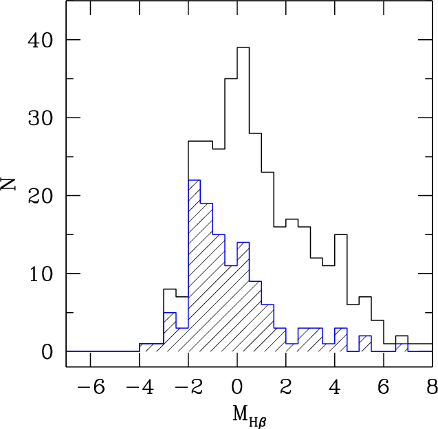
To illustrate this point, in Fig. 4 we show the luminosity function (PNLF) of Galactic PNe
in the H![]() -equivalent absolute magnitude. The H
-equivalent absolute magnitude. The H![]() fluxes are from Cahn et al. (1992), and the PN distances from Stanghellini et al. (2008; see also Stanghellini & Haywood 2010). The solid histogram represents the homogeneous Galactic sample of 331 PNe where both distance and H
fluxes are from Cahn et al. (1992), and the PN distances from Stanghellini et al. (2008; see also Stanghellini & Haywood 2010). The solid histogram represents the homogeneous Galactic sample of 331 PNe where both distance and H![]() flux are known, and where spectroscopy has been performed and a lower limit or a detection of the He II
flux are known, and where spectroscopy has been performed and a lower limit or a detection of the He II ![]() 4686 line has been acquired. The shaded histogram is the subsample
of Galactic PNe with
4686 line has been acquired. The shaded histogram is the subsample
of Galactic PNe with
![]() .
It is clear that at least 80-90
.
It is clear that at least 80-90![]() of the bright Galactic PNe do not show the He II lines, in qualitative agreement with not finding this emission line in the M 81 PN sample.
of the bright Galactic PNe do not show the He II lines, in qualitative agreement with not finding this emission line in the M 81 PN sample.
|
Figure 4:
The Galactic PNLF in the light of H |
| Open with DEXTER | |
In order to quantify the expectation of detecting the He II emission line in a given PN population of a certain metallicity we use Käufl et al.'s (1993) models to derive PN opacity, where the non-evolving term of the opacity,
![]() ,
scales directly with
the dust-to-gas ratio (see their Eq. (10)). We also express this ratio as expected at different metallicities,
,
scales directly with
the dust-to-gas ratio (see their Eq. (10)). We also express this ratio as expected at different metallicities,
![]() (O/H)/(O/H)
(O/H)/(O/H)![]() (Draine 2009),
where the right hand side term refers to the ratio of the oxygen vs.
hydrogen abundance in a given galaxy compared to that of the Milky Way.
To obtain the ratio for M 81 scaled to that of the Galaxy we use
the H II region oxygen abundances in M 81 (
(Draine 2009),
where the right hand side term refers to the ratio of the oxygen vs.
hydrogen abundance in a given galaxy compared to that of the Milky Way.
To obtain the ratio for M 81 scaled to that of the Galaxy we use
the H II region oxygen abundances in M 81 (
![]() )
and in the Galaxy (
)
and in the Galaxy (
![]() ,
Deharveng et al. 2000) to find
,
Deharveng et al. 2000) to find
![]() ,
thus for a given type of M 81 PN the thinning time would be
similar to that of the Galactic homologous. We conclude that the lack
of He II-emitting PNe in M 81 is totally expected, given the Galactic PNLF for both He II-emitting and non-emitting PNe (Fig. 4).
,
thus for a given type of M 81 PN the thinning time would be
similar to that of the Galactic homologous. We conclude that the lack
of He II-emitting PNe in M 81 is totally expected, given the Galactic PNLF for both He II-emitting and non-emitting PNe (Fig. 4).
It is interesting to compare the PN population of M 81 with that of M 33 as well. Magrini et al. (2010) obtained an average oxygen abundance of
![]() for H II regions in the M 33 disk, corresponding to a dust-to-mass ratio of
for H II regions in the M 33 disk, corresponding to a dust-to-mass ratio of ![]()
![]() ,
or, less than half that of M 81. By running the Käufl
et al.'s models for M 33 we obtain (Balmer line) thinning
times
,
or, less than half that of M 81. By running the Käufl
et al.'s models for M 33 we obtain (Balmer line) thinning
times ![]() 1.5 times shorter than in M 81 or the Galaxy, which can account for the relatively higher frequency of He II-emitting, bright PNe that where observed in M 33
by M09.
1.5 times shorter than in M 81 or the Galaxy, which can account for the relatively higher frequency of He II-emitting, bright PNe that where observed in M 33
by M09.
We know that the brightest PNe in a given population excludes the progeny of the
massive AGB stars, i.e., those with
![]() (Stanghellini & Renzini 2000).
The sample of M 81 PNe under study here thus does not include the
progeny of the more massive AGB stars. This agrees very well with the
observational fact that we do not
observe any type I PNe in our M 81 sample.
(Stanghellini & Renzini 2000).
The sample of M 81 PNe under study here thus does not include the
progeny of the more massive AGB stars. This agrees very well with the
observational fact that we do not
observe any type I PNe in our M 81 sample.
3 Radial metallicity gradients in M 81
3.1 The planetary nebula gradients
The metallicity gradient of a disk galaxy is generally intended as
the metallicity variation between the galactic center and the
periphery, measured radially. These gradients are essential constraints
for the chemical evolution models, and, depending on the probe, can
constrain the galactic composition at different times in evolution.
Planetary nebulae with low-mass progenitors, such as
non-type I PNe, probe the early stages of disk metallicity. We
could derive the metallicity gradients in M 81 from oxygen
abundances, thus probing the ![]() -element
evolution through the galactic disk. We estimate the distances of our
target PNe from the center of M 81 by using a rotation angle of 157
-element
evolution through the galactic disk. We estimate the distances of our
target PNe from the center of M 81 by using a rotation angle of 157![]() and an inclination of 59
and an inclination of 59![]() .
The error in the target coordinates is very low, and the major source of error in the distance calculation is the
uncertainty in the galaxy inclination, which we take as in Connolly et al. (1972),
.
The error in the target coordinates is very low, and the major source of error in the distance calculation is the
uncertainty in the galaxy inclination, which we take as in Connolly et al. (1972),
![]() ,
and we propagate to estimate the galactocentric distance uncertainties.
,
and we propagate to estimate the galactocentric distance uncertainties.
Table 6: Metallicity gradients.
|
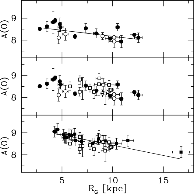
Figure 5: Oxygen abundances vs. galactocentric distances for M 81 targets. Top panel: the observed sample of PNe, with formal error bars and least square fit represented by solid line. Open symbols represent those PNe whose extinction constant might be overestimated. Middle panel: the H II region sample from MMT spectra (open squares) superimposed to the PN population of the top panel. Bottom panel: the H II regions from GS87 (filled squares) superimposed to the MMT H II regions of the middle panel (open squares). The line represents the least square fit for the combined sample, as given in Table 6. |
| Open with DEXTER | |
In Table 6, Cols. (3)
and (4), we give the metallicity gradients calculated for oxygen,
neon, and sulfur. Slopes are in dex kpc-1, while
intercepts are in dex, with the usual notation of A(X) = log(X/H) + 12.
In Fig. 5
(top panel) we show the oxygen gradient from the M 81 PNe, where
the line represent the linear fit. Only PNe are plotted in this top
panel, with filled symbols representing the general PN population, and
the open symbols indicating those PNe whose extinction correction from
the H![]() /H
/H![]() ratio does not well reproduce the line
intensity expected for the H
ratio does not well reproduce the line
intensity expected for the H![]() emission line. These open data points might thus have larger uncertainties than inferred from the formal
error analysis.
emission line. These open data points might thus have larger uncertainties than inferred from the formal
error analysis.
We perform the fits with the routine fitexy (see Numerical Recipes, Press et al. 1992) and
obtain
![]() dex kpc-1. Should we exclude the open symbols in the fit we would obtain a very similar result (
dex kpc-1. Should we exclude the open symbols in the fit we would obtain a very similar result (
![]() dex kpc-1).
dex kpc-1).
In Fig. 6 we show the metallicity gradients for sulfur (top) and neon (bottom), where the PNe are plotted with filled symbols. The solid lines represent the fits obtained with the fitexy routines that consider the formal errors both in abundances and distances (see Table 6). Fits obtained with the least square method are very similar.
3.2 H II regions in the A(X)-R plots
plots
The bottom panel of Fig. 5 shows the H II region analysis of oxygen abundances from this paper (open symbols) and from GS87 (filled symbols). Formal errorbars have
been applied to the data obtained in this paper, while in the case of the
GS87 sample we assume a 0.05![]() relative uncertainty in the distances, and a 0.25 dex uncertainty
in the oxygen abundances. It is worth noting that we have recalculated
the galactocentric distances for the GS87 targets by assuming the same
distance to M 81 than we use thorough this paper (d=3.63 Mpc) for homogeneity, although this does not affect the resulting gradient significantly.
The composite data sample has been fitted including the distance and abundances uncertainties with the fitexy routine, to give a gradient (
relative uncertainty in the distances, and a 0.25 dex uncertainty
in the oxygen abundances. It is worth noting that we have recalculated
the galactocentric distances for the GS87 targets by assuming the same
distance to M 81 than we use thorough this paper (d=3.63 Mpc) for homogeneity, although this does not affect the resulting gradient significantly.
The composite data sample has been fitted including the distance and abundances uncertainties with the fitexy routine, to give a gradient (
![]() dex kpc-1) not too dissimilar, yet steeper, from that of PNe. A direct least square fit would give a slightly milder gradient (
dex kpc-1) not too dissimilar, yet steeper, from that of PNe. A direct least square fit would give a slightly milder gradient (
![]() dex kpc-1). It is worth noting that both the average O/H abundance in H II regions
and the intercept of the linear metallicity gradient are consistently
higher that the respective values for PNe, as shown in Table 6, with PNe under abundant with respect to H II regions by almost a factor of 2, on average. This is well seen in the middle panel of Fig. 5, where PNe and H II regions from MMT observations are plotted together.
dex kpc-1). It is worth noting that both the average O/H abundance in H II regions
and the intercept of the linear metallicity gradient are consistently
higher that the respective values for PNe, as shown in Table 6, with PNe under abundant with respect to H II regions by almost a factor of 2, on average. This is well seen in the middle panel of Fig. 5, where PNe and H II regions from MMT observations are plotted together.
|
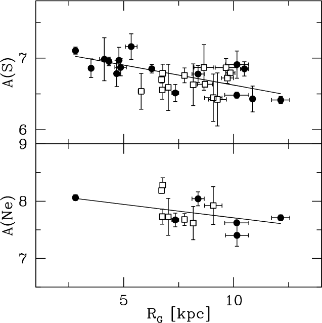
Figure 6: Sulfur (top panel) and neon (bottom panel) abundances from MMT observations vs. galactocentric distances for M 81 PNe (filled circles) and H II regions (open squares). The lines represent the linear fits to the PNe as discussed in the text. |
| Open with DEXTER | |
In Fig. 6 we show the sulfur (top) and neon (bottom) abundances in H II
regions versus their galactocentric distances (open symbols), plotted
together with the PN data (filled symbols). Since the H II regions
observed with the MMT span a small fraction of the galaxy radius,
metallicity gradients derived form these species would not be very
meaningful. Within the distance ranges populated by our H II region data we find
![]() ,
and
,
and
![]() .
Any further comparison is not sensible given the limited data at hand,
and we prefer to postpone a complete discussion of the sulfur and neon
abundances in PNe as compared to the H II regions of M 81 when more H II region spectral data with diagnostic lines relative to these atoms will be available.
.
Any further comparison is not sensible given the limited data at hand,
and we prefer to postpone a complete discussion of the sulfur and neon
abundances in PNe as compared to the H II regions of M 81 when more H II region spectral data with diagnostic lines relative to these atoms will be available.
4 Discussion
4.1 Galaxy evolution through oxygen abundances
The O/H abundances are among the most reliable in emission-line targets when only optical spectra are available. In the case of M 81, PNe and H II regions provide a meaningful comparison between young and old stellar objects, since the techniques of data acquisition, analysis, and abundance calculation are the same for both classes of objects. In particular, for several H II regions presented here, those observed with the MMT, the actual data acquisition is identical that that of the PNe, thus the comparison among data set is even more compelling.
It is worth emphasizing that the H II
region gradient is not based exclusively on our MMT data, which cover a
limited radial range, but also on the results by GS87. The
spectroscopic observations of GS87 did not allow a direct measurement
of the electron temperature. They derived ![]() by applying an indirect calibration made through the photoionization models by Pagel et al. (1979). The errors on the electron temperature are estimated of the order of
by applying an indirect calibration made through the photoionization models by Pagel et al. (1979). The errors on the electron temperature are estimated of the order of ![]() 1200 K, mainly due to the scatter of the measurements on which Pagel et al. (1979) based their calibrations. We have estimated, using the IRAF ionic task, that an uncertainty of
1200 K, mainly due to the scatter of the measurements on which Pagel et al. (1979) based their calibrations. We have estimated, using the IRAF ionic task, that an uncertainty of ![]() 1200 K in
1200 K in ![]() translates in
translates in ![]() 0.2 dex
in the ionic abundances. Thus, the chemical abundances of GS87 result
less accurate than ours, and may introduce biases in the determination
of the gradient. We conservatively have assumed uncertainties of
0.25 dex for the oxygen abundances from GS87.
0.2 dex
in the ionic abundances. Thus, the chemical abundances of GS87 result
less accurate than ours, and may introduce biases in the determination
of the gradient. We conservatively have assumed uncertainties of
0.25 dex for the oxygen abundances from GS87.
As shown in Fig. 5, the radial oxygen gradient slope of H II
regions is mildly steeper than that of PNe, with differences compatible
with the slope uncertainties. Since there are no type I PNe
in our sample it is sensible to assume that the PN progenitor (turnoff)
masses are smaller than ![]() 2
2 ![]() ,
implying a population older than
,
implying a population older than ![]() 1 Gyr (Maraston 1998). The lower limit for PN progenitor mass is around 1
1 Gyr (Maraston 1998). The lower limit for PN progenitor mass is around 1 ![]() ,
corresponding
to a galactic age of
,
corresponding
to a galactic age of ![]() 10 Gyr.
10 Gyr.
In Fig. 7 we plot the slope of the oxygen radial gradients in M 81 (squares) for PNe and H II regions, against the mean age of the population considered. H II regions are placed at t=0, while PN ages are inferred from the presumed mass of progenitors (see Stanghellini & Haywood 2010, for a detailed discussion of the different PN types). The horizontal error bar for PNe indicates the age range of the population, while all vertical error bars indicate the uncertainties in the slopes. It appears that the slope of the M 81 metallicity gradient did not vary very much during the past 10 Gyr. A flattening with time, as predicted by many chemical evolution models, is not supported by our observations. On the contrary, a constant slope, or a mild steepening of gradient slopes with time is inferred.

|
Figure 7: The slope of the oxygen gradients, in dex kpc-1, versus the age of the stellar population considered, for the Galaxy (filled circles, adapted from Stanghellini & Haywood 2010), M 33 (starred symbols, adapted from M09 and M10) and M 81 (squares, this paper). The zero-age populations represent the slopes of the gradients estimated though H II region oxygen abundances, while all other points are slopes of PN gradients, see text. Error-bars in the x direction represent the approximate age span of the populations, and in the y direction are the estimated metallicity uncertainties. The zero-age data point for M 81 is uncertain, as it is based on the combination of of the H II regions observed with the MMT and the GS87 sample. |
| Open with DEXTER | |
While uncertainties in the actual slopes are high, it is worth comparing the results of M 81 with what found in M 33 PNe and H II regions (M09 and M10, starred symbols), and the Milky Way (PNe from Stanghellini & Haywood 2010; H II regions from Deharveng et al. 2000, filled circles). The metallicity gradients are generally steeper in M 81 than in either the Milky Way and M 33, but in all three galaxies we observe mild flattening with the age of the population, going from steeper for H II regions to flatter for non-type I PNe. It is worth noting that in the Galaxy the PN types I, II, and III were independently selected to calculate the oxygen radial gradients, while in M 33 we were able to distinguish between type I and non-type I.
Since the gradient slopes seem to flatten with the age of the population considered, there is an indication that the gradients themselves are steepening with the galaxy age in all the three galaxies considered. It is a mild steepening, and with large uncertainties, but it is consistently found in all three galaxies, so it is worth exploring it.
Let us recall that the slope of the H II gradient in M 33 excluded the central kpc, as explained by M 10. If we were including H II regions in the central kpc we would obtain nearly no gradient evolution between H II
regions and type I PNe in M 33. There is thus some evolution
of the oxygen gradients with time, where the slopes vary by
![]() to
to ![]()
![]() dex per radial kpc in
dex per radial kpc in ![]() 10 Gyr. Stanghellini & Haywood (2010)
offer the hypothesis that portions of the Milky Way at different radial
distances might have evolved at different rates. The model by Schönrich
& Binney (2009) illustrates this type of evolution,
which could hold as well for the other spiral galaxies and for M 81.
10 Gyr. Stanghellini & Haywood (2010)
offer the hypothesis that portions of the Milky Way at different radial
distances might have evolved at different rates. The model by Schönrich
& Binney (2009) illustrates this type of evolution,
which could hold as well for the other spiral galaxies and for M 81.
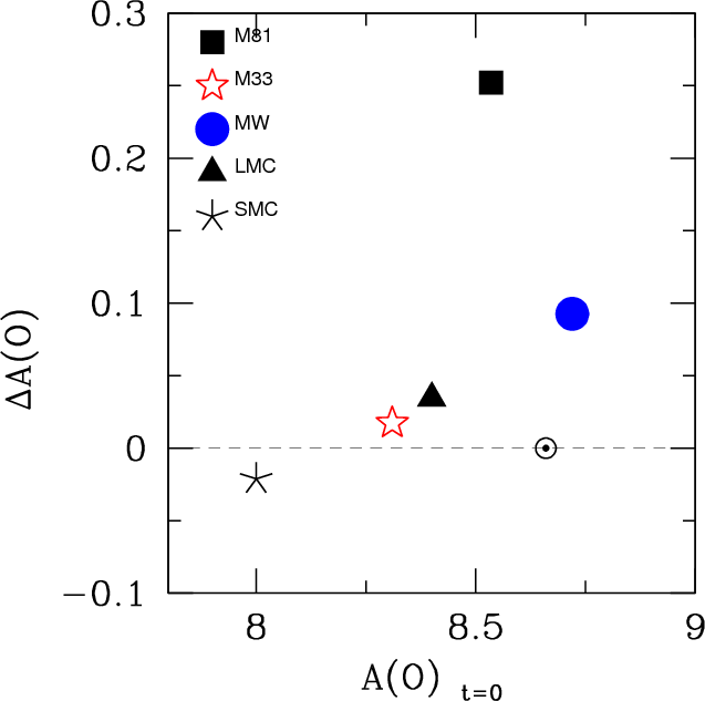
In Fig. 8 we show the global oxygen evolution in different galaxies, where average oxygen abundances in H II regions are plotted against the same quantities in non-type I PNe. In the case of the disk galaxies, both populations cover a reasonable radial range and are representative of the whole disks. The SMC and LMC oxygen abundance are from Leisy & Dennefeld (2006), and the H II regions in the Magellanic Clouds are from Dennefeld (1989). The samples of PNe and H II regions considered in the Galaxy and M 33 are as described earlier in this section. M 81 PN and H II regions abundances are from this paper, both selected consistently within the galactocentric distance domain where both sets of targets coexist. The solar point is from Asplund et al. (2005). In this plot M 81 stands out as the galaxy with most chemical enrichment in the group considered. M 33, as found by M10, shows almost no enrichment, and the other galaxies show either low enrichment (the Galaxy and the LMC) or slight depletion of oxygen in the SMC, where the cause could be extremely efficient ON cycle at very low metallicity (Karakas & Lattanzio 2007). The average enrichment of M 81 is 0.25 dex.
|
Figure 8: Difference between average oxygen abundance of H II regions and non-type I PNe vs. zero-age average oxygen abundance for M 81 (square, this paper), compared to that of M 33 (starred symbol, M09 and M10), the Magellanic Clouds (LMC: triangle, SMC: diamond; Garnett 1999; M09), and the Milky Way (filled circle, Stanghellini & Haywood 2010; Peimbert 1999). The solar value represented is from Asplund et al. (2005). The M 81 datum is derived from PN and H II regions in the 5.8-9.8 kpc range, and does not include the GS87 data. The M 81 galaxy shows considerable metal enrichment. |
| Open with DEXTER | |
The M 81 galaxy disk shows indication of chemical enrichment through oxygen abundances. It also shows generally steeper metallicity gradients than both M 33 and the Galaxy. The non-type I PNe gradients in M 81 is - 0.055 dex kpc-1, while homologous slopes are -0.03 and -0.02 dex kpc-1 respectively in M 33 and the Galaxy, indicating that whatever process produces the metallicity gradients in spiral galaxies, it is more efficient in M 81 and the overall galaxy metallicity is not a factor. Similarly for H II regions, the M 81 gradient slope is -0.09 dex kpc-1, to be compared with -0.044 and -0.04 dex kpc-1 for M 33 and the Milky Way respectively. Indication of steeper gradients, and sizable chemical evolution, are thus the defining characteristics of M 81 compared with other spirals. The oxygen enrichment indicates that this galaxy has suffered outflow to a lesser extent than the comparison galaxies, and steeper oxygen gradients are compatible with this explanation.
Table 7: Properties of M 81 and the Galaxy.
4.2 The chemical evolution of M 81: comparison with the Milky Way
It is evident from the above analysis that the metallicity gradient slopes in the galaxies examined do not depend on the average galactic metallicity: M 33 is metal poor (its metallicity is similar to that of the LMC, Leisy & Dennefeld 2006) and M 81 is closer in metal contents to the Galaxy. Since M 81 is also closer to the Galaxy in stellar mass content (see Table 7 for a direct comparison of the main properties of these two galaxies), it makes sense to compare these two galaxies directly, to explore the relations of the metallicity gradients to the characteristics of the galaxy disks and to their evolution. The observations of PNe tell us that the gradient of M 81 is steeper than that of our Galaxy in old stellar populations; the trend seems to persist in the young stellar population, but this needs further confirmation.
From a theoretical point of view, there are two main reasons that could influence the gradient slopes, (1) the rotational velocity of the galaxy and (2) the different situation of these two galaxies within their environment.
Mollá & Diaz (2005) noted that metallicity gradients depend on the rotational velocity of the galaxy (thus presumably on its total mass), and on its morphological type: more massive galaxies tend to evolve faster and have flatter gradients than lower mass galaxies; for a given rotation velocity, gradients are steeper for late type than for early type galaxies. Both effects would imply a steeper gradient for the Galaxy than for M 81, contrary to the observations. Some other factor must be at play.
It is likely that the situation of M 81 within its group of galaxies influences its metallicity gradient. The tidal H I features near M 81 are consistent with a large-scale redistribution of gas in this galaxy. M 81 is the only massive galaxy of its group, surrounded by several small galaxies. The interaction of M 81 with the dwarf galaxies of its group probably steepens the gradient of the major member due to the effect of stripping gas from the external regions of the major companion, while interaction of galaxies with more or less the same mass would redistribute the gas in both galaxies, and thus flatten the gradient.
The chemical evolution models of Valle et al. (2005) consider the
effects of gas stripping due to galaxy encounters on the star formation
rate and the evolution of the metallicity. They found that, for a
stripping occurring 1-3 Gyr after the formation of the galaxy and
removing 97![]() of the gas, the region affected by the gas removal has
a SFR almost a factor of 10 lower than in the model without stripping
and the relative metallicity is then reduced by about 40
of the gas, the region affected by the gas removal has
a SFR almost a factor of 10 lower than in the model without stripping
and the relative metallicity is then reduced by about 40![]() .
The
metallicity reduction is not strongly dependent on the time and
duration of the stripping episode, but is quite sensitive to the
relative amount of gas removed from the region. This effect should be
more pronounced in the outer than the inner galactic regions, due to
the proximity of the interacting galaxies, and it might explain why M 81
has steeper metallicity gradients than the Galaxy. Unfortunately, the
models by Valle et al. (2005) are limited to a single radial region,
thus this conclusion is of qualitative nature. A radially-resolved
chemical evolution modeling taking into account the effects of
stripping would be necessary to determine the effect of tidal
interaction on the gradient, and also to compare with other results.
.
The
metallicity reduction is not strongly dependent on the time and
duration of the stripping episode, but is quite sensitive to the
relative amount of gas removed from the region. This effect should be
more pronounced in the outer than the inner galactic regions, due to
the proximity of the interacting galaxies, and it might explain why M 81
has steeper metallicity gradients than the Galaxy. Unfortunately, the
models by Valle et al. (2005) are limited to a single radial region,
thus this conclusion is of qualitative nature. A radially-resolved
chemical evolution modeling taking into account the effects of
stripping would be necessary to determine the effect of tidal
interaction on the gradient, and also to compare with other results.
5 Conclusions
Hectospec/MMT spectroscopy of a sizable sample of PN and H II
regions in the nearby M 81 galaxy has proven very efficient to
find chemistry of the young and old stellar populations, and to pin
point the radial metallicity gradients. We were able to detect the
diagnostic lines for plasma and abundance analysis in 19 PNe and
14 H II regions. Their analysis indicates that the galaxy is clearly chemically enriched, with
![]() /
/
![]() ,
from MMT spectra where PNe and H II regions were simultaneously acquired.
We also found that there is a noticeable PN metallicity gradient in oxygen, with
,
from MMT spectra where PNe and H II regions were simultaneously acquired.
We also found that there is a noticeable PN metallicity gradient in oxygen, with
![]() dex kpc-1, and that
neon and sulfur gradient slopes are within 15
dex kpc-1, and that
neon and sulfur gradient slopes are within 15![]() of the oxygen one. The MMT sample of H II
regions have limited galactocentric distribution, thus they are
insufficient probes of the metallicity gradient. The gradient slope
from the combined MMT and GS87 H II region samples
is steeper (-0.093 dex kpc-1)
than that of the PNe, possibly indicating an evolution of the radial
metallicity gradients with time: older stellar population
show shallower gradients, thus gradients are steepening with the time
since galaxy formation. These results have been compared to their
homologous
for the Milky Way and M 33, where similar (yet less marked)
gradient steepening is inferred.
We plan to increase the size of the H II region
sample, and to extend their gradient study to other atoms such as neon
and sulfur in the near future, for
a more complete comparison with the PNe, with the goal of obtaining
firmer observational constraints for the chemical evolutionary models.
of the oxygen one. The MMT sample of H II
regions have limited galactocentric distribution, thus they are
insufficient probes of the metallicity gradient. The gradient slope
from the combined MMT and GS87 H II region samples
is steeper (-0.093 dex kpc-1)
than that of the PNe, possibly indicating an evolution of the radial
metallicity gradients with time: older stellar population
show shallower gradients, thus gradients are steepening with the time
since galaxy formation. These results have been compared to their
homologous
for the Milky Way and M 33, where similar (yet less marked)
gradient steepening is inferred.
We plan to increase the size of the H II region
sample, and to extend their gradient study to other atoms such as neon
and sulfur in the near future, for
a more complete comparison with the PNe, with the goal of obtaining
firmer observational constraints for the chemical evolutionary models.
The observations reported here were obtained at the MMT Observatory, a facility operated jointly by the Smithsonian Institution and the University of Arizona. MMT telescope time was granted by NOAO, through the Telescope System Instrumentation Program (TSIP). TSIP is funded by NSF. We warmly thank D. Fabricant for making Hectospec available to the community, and the Hectospec instrument team and MMT staff for their expert help in preparing and carrying out the Hectospec observing runs. We thank N. Caldwell, D. Ming, and their team for the help during the data reduction. L.S. acknowledges the Observatoire de Paris and the Osservatorio Astrofisico di Arcetri for their hospitality during different stages of this project.
References
- Appleton, P. N., Davies, R. D., & Stephenson, R. J. 1981, MNRAS, 195, 327 [NASA ADS] [CrossRef] [Google Scholar]
- Asplund, M., Grevesse, N., & Sauval, A. J. 2005, Cosmic Abundances as Records of Stellar Evolution and Nucleosynthesis, 336, 25 [NASA ADS] [Google Scholar]
- Benjamin, R. A., Skillman, E. D., & Smits, D. P. 1999, ApJ, 514, 307 [NASA ADS] [CrossRef] [Google Scholar]
- Cahn, J. H., Kaler, J. B., & Stanghellini, L. 1992, A&AS, 94, 399 [NASA ADS] [Google Scholar]
- Clegg, R. E. S. 1987, MNRAS, 229, 31 [NASA ADS] [CrossRef] [Google Scholar]
- Connolly, L. P., Mantarakis, P. Z., & Thompson, L. A. 1972, PASP, 84, 61 [NASA ADS] [CrossRef] [Google Scholar]
- Davidge, T. J. 2009, ApJ, 697, 1439 [NASA ADS] [CrossRef] [Google Scholar]
- Deharveng, L., Pena, M., Caplan, J., & Costero, R. 2000, MNRAS, 311, 329 [NASA ADS] [CrossRef] [Google Scholar]
- Dennefeld, M. 1989, Recent Developments of Magellanic Cloud Research, 107 [Google Scholar]
- Dors, O. L., Jr., & Copetti, M. V. F. 2006, A&A, 452, 473 [Google Scholar]
- Draine, B. T. 2009, EAS Publications Series, 35, 245 [CrossRef] [EDP Sciences] [Google Scholar]
- Fabricant, D., Fata, R., Roll, J., et al. 2005, PASP, 117, 1411 [NASA ADS] [CrossRef] [Google Scholar]
- Freedman, W. L., Madore, B. F., Gibson, B. K., et al. 2001, ApJ, 553, 47 [NASA ADS] [CrossRef] [Google Scholar]
- Garnett, D. R. 1999, New Views of the Magellanic Clouds, 190, 266 [NASA ADS] [Google Scholar]
- Garnett, D. R., & Shields, G. A. 1987, ApJ, 317, 82 (GS87) [NASA ADS] [CrossRef] [Google Scholar]
- Gordon, K. D., Pérez-González, P. G., Misselt, K. A., et al. 2004, ApJS, 154, 215 [NASA ADS] [CrossRef] [Google Scholar]
- Gottesman, S. T., & Weliachew, L. 1975, ApJ, 195, 23 [NASA ADS] [CrossRef] [Google Scholar]
- Henry, R. B. C., Kwitter, K. B., & Balick, B. 2004, AJ, 127, 2284 [NASA ADS] [CrossRef] [Google Scholar]
- Hodge, P., & Miller, B. 1992, BAAS, 24, 1201 [NASA ADS] [Google Scholar]
- Hodge, P. W., & Kennicutt, R. C., Jr. 1983, AJ, 88, 296 [NASA ADS] [CrossRef] [Google Scholar]
- Jacoby, G. H., Ciardullo, R., Booth, J., & Ford, H. C. 1989, ApJ, 344, 704 [NASA ADS] [CrossRef] [Google Scholar]
- Käufl, H. U., Renzini, A., & Stanghellini, L. 1993, ApJ, 410, 251 [NASA ADS] [CrossRef] [Google Scholar]
- Karakas, A., & Lattanzio, J. C. 2007, Publications of the Astronomical Society of Australia, 24, 103 [Google Scholar]
- Karachentsev, I. D., & Kashibadze, O. G. 2006, Astrophysics, 49, 3 [NASA ADS] [CrossRef] [Google Scholar]
- Kingsburgh, R. L., & Barlow, M. J. 1994, MNRAS, 271, 257 [NASA ADS] [CrossRef] [Google Scholar]
- Kong, X., Zhou, X., Chen, J., et al. 2000, AJ, 119, 2745 [NASA ADS] [CrossRef] [Google Scholar]
- Leisy, P., & Dennefeld, M. 2006, A&A, 456, 451 [NASA ADS] [CrossRef] [EDP Sciences] [Google Scholar]
- Lin, W., Zhou, X., Burstein, D., et al. 2003, AJ, 126, 1286 [NASA ADS] [CrossRef] [Google Scholar]
- Maciel, W. J., & Quireza, C. 1999, A&A, 345, 629 [NASA ADS] [Google Scholar]
- Magrini, L., Perinotto, M., Corradi, R. L. M., & Mampaso, A. 2001, A&A, 379, 90 [NASA ADS] [CrossRef] [EDP Sciences] [Google Scholar]
- Magrini, L., Corbelli, E., & Galli, D. 2007, A&A, 470, 843 [NASA ADS] [CrossRef] [EDP Sciences] [Google Scholar]
- Magrini, L., Stanghellini, L., & Villaver, E. 2009, ApJ, 696, 729 (M09) [NASA ADS] [CrossRef] [Google Scholar]
- Magrini, L., Stanghellini, L., Corbelli, E., Galli, D., & Villaver, E. 2010, A&A, 512, A63 (M10) [NASA ADS] [CrossRef] [EDP Sciences] [Google Scholar]
- Marigo, P. 2001, A&A, 370, 194 [NASA ADS] [CrossRef] [EDP Sciences] [Google Scholar]
- Massey, P., Strobel, K., Barnes, J. V., & Anderson, E. 1988, ApJ, 328, 315 [NASA ADS] [CrossRef] [Google Scholar]
- Mathis, J. S. 1990, ARA&A, 28, 37 [NASA ADS] [CrossRef] [Google Scholar]
- Maraston, C. 1998, MNRAS, 300, 872 [NASA ADS] [CrossRef] [Google Scholar]
- Mollá, M., & Díaz, A. I. 2005, MNRAS, 358, 521 (MD05) [NASA ADS] [CrossRef] [Google Scholar]
- Osterbrock, D. E., & Ferland, G. J. 2006, Astrophysics of gaseous nebulae and active galactic nuclei, 2nd. edn., ed. D.E. Osterbrock, & G.J. Ferland (Sausalito, CA: University Science Books) [Google Scholar]
- Pagel, B. E. J., Edmunds, M. G., Blackwell, D. E., Chun, M. S., & Smith, G. 1979, MNRAS, 189, 95 [NASA ADS] [CrossRef] [Google Scholar]
- Peimbert, M. 1999, Chemical Evolution from Zero to High Redshift, 30 [Google Scholar]
- Peimbert, M., & Torres-Peimbert, S. 1983, in Proc. Symp. (Dordrecht: D. Reidel Publishing Co.), 233 [Google Scholar]
- Perinotto, M., & Morbidelli, L. 2006, MNRAS, 372, 45 [NASA ADS] [CrossRef] [Google Scholar]
- Perinotto, M., Morbidelli, L., & Scatarzi, A. 2004, MNRAS, 349, 793 [NASA ADS] [CrossRef] [Google Scholar]
- Press, W. H., Teukolsky, S. A., Vetterling, W. T., & Flannery, B. P. 1992, (Cambridge: University Press), 2nd edn. [Google Scholar]
- Rohlfs, K., & Kreitschmann, J. 1980, A&A, 87, 175 [NASA ADS] [Google Scholar]
- Sabbi, E., Gallagher, J. S., Smith, L. J., de Mello, D. F., & Mountain, M. 2008, ApJL, 676, L113 [NASA ADS] [CrossRef] [Google Scholar]
- Shaw, R. A., & Dufour, R. J. 1994, ASPC, 61, 327 [Google Scholar]
- Schönrich, R., & Binney, J. 2009, MNRAS, 396, 203 [NASA ADS] [CrossRef] [Google Scholar]
- Stanghellini, L., & Kaler, J. B. 1989, ApJ, 343, 811 [NASA ADS] [CrossRef] [Google Scholar]
- Stanghellini, L., & Renzini, A. 2000, ApJ, 542, 308 [NASA ADS] [CrossRef] [Google Scholar]
- Stanghellini, L., & Haywood, M. 2010, ApJ, 714, 1096 [NASA ADS] [CrossRef] [Google Scholar]
- Stanghellini, L., Guerrero, M. A., Cunha, K., Manchado, A., & Villaver, E. 2006, ApJ, 651, 898 [NASA ADS] [CrossRef] [Google Scholar]
- Stanghellini, L., Shaw, R. A., & Villaver, E. 2008, ApJ, 689, 194 [NASA ADS] [CrossRef] [EDP Sciences] [Google Scholar]
- Valle, G., Shore, S. N., & Galli, D. 2005, A&A, 435, 551 [NASA ADS] [CrossRef] [EDP Sciences] [Google Scholar]
- van der Kruit, P. C. 1990, The Milky Way as a Galaxy, 331 [Google Scholar]
- Walterbos, R. A. M., & Braun, R. 1994, ApJ, 431, 156 [NASA ADS] [CrossRef] [Google Scholar]
- Villaver, E., Manchado, A., & García-Segura, G. 2002, ApJ, 581, 1204 [NASA ADS] [CrossRef] [Google Scholar]
- Weisz, D. R., Skillman, E. D., Cannon, J. M., et al. 2008, ApJ, 689, 160 [NASA ADS] [CrossRef] [Google Scholar]
- Yun, M. S., Ho, P. T. P., & Lo, K. Y. 1994, Nature, 372, 530 [NASA ADS] [CrossRef] [PubMed] [Google Scholar]
- Yun, M. S. 1999, Galaxy Interactions at Low and High Redshift, 186, 81 [Google Scholar]
- Zaritsky, D., Kennicutt, R. C., Jr., & Huchra, J. P. 1994, ApJ, 420, 87 [NASA ADS] [CrossRef] [Google Scholar]
Footnotes
- ... evolution
- Full Tables 2 and 3 are only available in electronic form at the CDS via anonymous ftp to cdsarc.u-strasbg.fr (130.79.128.5) or via http://cdsarc.u-strasbg.fr/viz-bin/qcat?J/A+A/521/A3
- ... IRAF
- IRAF is distributed by the National Optical Astronomy Observatory, which is operated by the Association of Universities for Research in Astronomy (AURA) under cooperative agreement with the National Science Foundation.
All Tables
Table 1: Observing log.
Table 2: Observed fluxes and line intensities.
Table 3: Plasma analysis and abundances.
Table 4: Temperatures and abundances uncertainties.
Table 5: Galactocentric distances and elemental abundances.
Table 6: Metallicity gradients.
Table 7: Properties of M 81 and the Galaxy.
All Figures
|
|
Figure 1: Sample of medium-resolution spectra of M 81 PNe. |
| Open with DEXTER | |
| In the text | |
|
|
Figure 2: The log(S2+/log(S+) versus log(O2+/log(O+) correlation (solid line), based on the Galactic PNe from Kingsburgh & Barlow (1994, open circles). Our targets are shown with filled circles. |
| Open with DEXTER | |
| In the text | |
|
|
Figure 3: log (N/O) vs. He/H; broken lines show He/H = .125 and log(N/O) = -0.3. Type I PNe would be located in the upper-right quadrant. |
| Open with DEXTER | |
| In the text | |
|
|
Figure 4:
The Galactic PNLF in the light of H |
| Open with DEXTER | |
| In the text | |
|
|
Figure 5: Oxygen abundances vs. galactocentric distances for M 81 targets. Top panel: the observed sample of PNe, with formal error bars and least square fit represented by solid line. Open symbols represent those PNe whose extinction constant might be overestimated. Middle panel: the H II region sample from MMT spectra (open squares) superimposed to the PN population of the top panel. Bottom panel: the H II regions from GS87 (filled squares) superimposed to the MMT H II regions of the middle panel (open squares). The line represents the least square fit for the combined sample, as given in Table 6. |
| Open with DEXTER | |
| In the text | |
|
|
Figure 6: Sulfur (top panel) and neon (bottom panel) abundances from MMT observations vs. galactocentric distances for M 81 PNe (filled circles) and H II regions (open squares). The lines represent the linear fits to the PNe as discussed in the text. |
| Open with DEXTER | |
| In the text | |
|
|
Figure 7: The slope of the oxygen gradients, in dex kpc-1, versus the age of the stellar population considered, for the Galaxy (filled circles, adapted from Stanghellini & Haywood 2010), M 33 (starred symbols, adapted from M09 and M10) and M 81 (squares, this paper). The zero-age populations represent the slopes of the gradients estimated though H II region oxygen abundances, while all other points are slopes of PN gradients, see text. Error-bars in the x direction represent the approximate age span of the populations, and in the y direction are the estimated metallicity uncertainties. The zero-age data point for M 81 is uncertain, as it is based on the combination of of the H II regions observed with the MMT and the GS87 sample. |
| Open with DEXTER | |
| In the text | |
|
|
Figure 8: Difference between average oxygen abundance of H II regions and non-type I PNe vs. zero-age average oxygen abundance for M 81 (square, this paper), compared to that of M 33 (starred symbol, M09 and M10), the Magellanic Clouds (LMC: triangle, SMC: diamond; Garnett 1999; M09), and the Milky Way (filled circle, Stanghellini & Haywood 2010; Peimbert 1999). The solar value represented is from Asplund et al. (2005). The M 81 datum is derived from PN and H II regions in the 5.8-9.8 kpc range, and does not include the GS87 data. The M 81 galaxy shows considerable metal enrichment. |
| Open with DEXTER | |
| In the text | |
Copyright ESO 2010
Current usage metrics show cumulative count of Article Views (full-text article views including HTML views, PDF and ePub downloads, according to the available data) and Abstracts Views on Vision4Press platform.
Data correspond to usage on the plateform after 2015. The current usage metrics is available 48-96 hours after online publication and is updated daily on week days.
Initial download of the metrics may take a while.