| Issue |
A&A
Volume 521, October 2010
|
|
|---|---|---|
| Article Number | A17 | |
| Number of page(s) | 12 | |
| Section | Catalogs and data | |
| DOI | https://doi.org/10.1051/0004-6361/200913979 | |
| Published online | 14 October 2010 | |
GASS: the Parkes Galactic all-sky survey
II. Stray-radiation correction and second data release
P. M. W. Kalberla1 -
N. M. McClure-Griffiths2 -
D. J. Pisano3,10,![]() -
M. R. Calabretta2 -
H. Alyson Ford2,5,9 -
F. J. Lockman4 -
L. Staveley-Smith6 -
J. Kerp1 -
B. Winkel1 -
T. Murphy7,8 -
K. Newton-McGee2,8
-
M. R. Calabretta2 -
H. Alyson Ford2,5,9 -
F. J. Lockman4 -
L. Staveley-Smith6 -
J. Kerp1 -
B. Winkel1 -
T. Murphy7,8 -
K. Newton-McGee2,8
1 - Argelander-Institut für Astronomie, Universität Bonn, Auf dem Hügel 71, 53121 Bonn, Germany
2 -
Australia Telescope National Facility, CSIRO, Marsfield NSW 2122, Australia
3 -
Department of Physics, West Virginia University, PO Box 6315, Morgantown, WV 26506, USA
4 -
National Radio Astronomy Observatory, Green Bank, WV 24944, USA
5 -
Centre for Astrophysics and Supercomputing, Swinburne University of Technology, Hawthorn VIC 3122, Australia
6 -
International Centre for Radio Astronomy Research, M468, University of Western Australia, Crawley, WA 6009, Australia
7 -
School of Physics, The University of Sydney, NSW 2006, Australia
8 -
School of Information Technologies, The University of Sydney, NSW 2006, Australia
9 -
Department of Astronomy, University of Michigan, Ann Arbor, MI 48109, USA
Received 28 December 2009 / Accepted 1 July 2010
Abstract
Context. The Parkes Galactic all-sky survey (GASS) is a survey of Galactic atomic hydrogen (H I)
emission in the southern sky observed with the Parkes 64-m Radio
Telescope. The first data release was published by McClure-Griffiths
et al. (2009).
Aims. We remove instrumental effects that affect the GASS and present the second data release.
Methods. We calculate the stray-radiation by convolving the
all-sky response of the Parkes antenna with the brightness temperature
distribution from the Leiden/Argentine/Bonn (LAB) all sky 21-cm line
survey, with major contributions from the 30-m dish of the Instituto
Argentino de Radioastronomía (IAR) in the southern sky. Remaining
instrumental baselines are corrected using the LAB data for a first
guess of emission-free baseline regions. Radio frequency interference
is removed by median filtering.
Results. After applying these corrections to the GASS we find an
excellent agreement with the Leiden/Argentine/Bonn (LAB) survey. The
GASS is the highest spatial resolution, most sensitive, and is
currently the most accurate H I survey of the Galactic H I emission in the southern sky. We provide a web interface for generation and download of FITS cubes.
Key words: surveys - ISM: general - radio lines: ISM - Galaxy: structure
1 Introduction
Atomic hydrogen (H I) is ubiquitous, it traces the interstellar medium (ISM) in disk galaxies over a broad range of physical conditions. Its 21-cm emission line is a key probe of the structure and dynamics of galaxies over a broad range of different densities and temperatures. H I is the key element to understand the evolution of the ISM in general (Kalberla & Kerp 2009). 21-cm line observations of the Milky Way are of particular interest because small scale structures are observable which can not be resolved with observations of any other galaxy. A number of notable items have been detailed by McClure-Griffiths et al. (2009, hereafter Paper I), this includes the impact of massive stars on the ISM, the disk-halo interaction, the ISM life-cycle and the formation of cold clouds. H I is a perfect tracer of the Galactic structure and there is a good correlation between gas and dust (Schlegel et al. 1998).
Table 1: Survey parameters for major single dish surveys of the Galactic 21-cm line emission. GALFA-HI and EBHIS are still in progress.
Galactic H I data are important for an exploration of the early universe
because of the photoelectric absorption caused by the ISM in the soft X-ray
energy range below 1 keV. The attenuation of the X-rays by the Galactic
interstellar medium increases with decreasing X-ray energy
(Kerp 2003). The emission of active Galactic nuclei at high redshifts (![]() )
or the faint emission of clusters of galaxies at moderate redshifts
(
)
or the faint emission of clusters of galaxies at moderate redshifts
(
![]() )
is shifted to this soft X-ray band. It is not possible to
analyze the X-ray data quantitatively without knowing in detail the
distribution of the Galactic interstellar medium across the target.
)
is shifted to this soft X-ray band. It is not possible to
analyze the X-ray data quantitatively without knowing in detail the
distribution of the Galactic interstellar medium across the target.
High resolution single dish data are needed but neither the H I Parkes All Sky Survey (HIPASS) by Barnes et al. (2001) nor the reprocessed version (HIPASS-HVC) by Putman et al. (2002) provide accurate column densities for the Galactic emission in the southern sky. The GASS provides such data. For the northern sky the Galactic Arecibo L-Band Feed H I (GALFA-HI) survey (Peek & Heiles 2008) and the Effelsberg-Bonn H I Survey (EBHIS) are still in progress (Winkel et al. 2010). Major parameters for these surveys are compared in Table 1. Currently the LAB and the GASS are the only surveys that are easily accessible for data mining.
The Galactic All-Sky Survey (GASS) is a 21-cm line survey covering the
southern sky for all declinations
![]() .
The observations were
made with the multibeam system on the 64-m Parkes Radio Telescope. The
intrinsic angular resolution of the data is
.
The observations were
made with the multibeam system on the 64-m Parkes Radio Telescope. The
intrinsic angular resolution of the data is
![]() (FWHM). The velocity
resolution is 1.0 km s-1 and the useful bandpass covers a velocity range
(FWHM). The velocity
resolution is 1.0 km s-1 and the useful bandpass covers a velocity range
![]() km s-1 for all of the observations; some data cover up to
km s-1 for all of the observations; some data cover up to
![]() km s-1. The GASS is the most sensitive, highest
angular resolution large-scale survey of Galactic H I emission ever made in
the southern sky. The first data release is available at
http://www.atnf.csiro.au/research/GASS.
km s-1. The GASS is the most sensitive, highest
angular resolution large-scale survey of Galactic H I emission ever made in
the southern sky. The first data release is available at
http://www.atnf.csiro.au/research/GASS.
A detailed description of the GASS project, focusing on the survey goals and techniques has been given by Naomi2009. In Paper I all of the initial data reduction and imaging is described in detail. Here we focus on the post-processing, in particular on corrections for stray-radiation, instrumental baselines, and radio frequency interference (RFI). We will note where our data reduction differs from that described in Naomi2009.
For 21-cm line observations there are a few unavoidable instrumental issues that can potentially degrade the data. The first is that a radio telescope does not have a perfect beam, so some radiation enters through the sidelobes of the antenna, causing spurious emission features. The second effect is that the receiver gain may drift, and it can suffer from instrumental spectral structure (the instrumental baseline) that may be time-dependent. These influences need to be minimized, but the raw observations do not allow a clear identification and separation of individual instrumental problems. For example, spurious profile wings may be caused by stray-radiation but also by instrumental baseline defects. Temporal fluctuations in the line emission may be due to gain variations but may also be caused by spurious emission from the sidelobes.
A strategy is needed to disentangle these instrumental issues. For the
stray-radiation correction a basic prerequisite is the knowledge of the H I
brightness temperature distribution provided by the Leiden/Argentine/Bonn
(LAB) 21-cm line survey (Kalberla et al. 2005); most important in the context of
the GASS survey is the contribution from the 30-m dish of the Instituto
Argentino de Radioastronomía (IAR) in the southern sky
(Bajaja et al. 2005). These surveys provide clean data with an angular
resolution of ![]()
![]() and allow us to solve the Fredholm integral
equation which describes the deconvolution of the raw observations (antenna
temperatures) with respect to the influences of the antenna
response. Bootstrapping from the LAB survey we use a model of the antenna
response for the 13-beam receiver based on the known feed patterns and the
telescope geometry. Section 2 describes how spurious features from the
sidelobes are removed.
and allow us to solve the Fredholm integral
equation which describes the deconvolution of the raw observations (antenna
temperatures) with respect to the influences of the antenna
response. Bootstrapping from the LAB survey we use a model of the antenna
response for the 13-beam receiver based on the known feed patterns and the
telescope geometry. Section 2 describes how spurious features from the
sidelobes are removed.
Next we remove baseline defects. For this the LAB survey is used for initial estimates of velocity ranges that do not contain line emission. In Sect. 3 we describe how baselines are refined in an iterative way. A gain calibration requires some preliminary baseline corrections but such a calibration also affects the accuracy of the corrections for stray-radiation. The calibration is described in Sect. 4. All corrections discussed in Sects. 2 to 4 need to be iterated several times.
RFI is increasingly a problem for sensitive observations, and post-processing mitigation strategies are essential. We use flags which were set in the first stage of the data processing by Livedata described in Naomi2009 and iteratively remove the remaining interference as discussed in Sect. 5. Throughout the reduction we take care that the corrections described in Sects. 2 to 4 are not affected by RFI.
In comparison with the LAB survey, the GASS represents an improvement in velocity resolution and sensitivity, but most important is the enhanced spatial resolution (Table 1). The generation of FITS images with user-definable parameters is described in Sect. 6. We discuss some examples of the newly corrected data in Sect. 7 and complete the paper with a description of a web interface for download (Sect. 8).
2 The stray-radiation correction
A major problem when observing 21-cm emission lines is caused by the fact that Galactic emission is seen in all directions. Most prominent is the bright Galactic plane which extends across the whole sky. It is unavoidable that stray 21-cm emission from the plane will get picked up by sidelobes of the antenna. The main sidelobes are the result of reflections from the feed legs that carry the prime focus cabin. Also radiation originating from regions outside the rim of the reflector, the spillover region, is received. Stray-radiation varies with time (van Woerden 1962) and for positions with very low H I the spurious emission features may amount to 50% of the total received signal (Hartmann et al. 1996; Kalberla et al. 1980a; Lockman et al. 1986). In some GASS spectra stray-radiation was found to comprise 35% of the observed emission.
Stray-radiation may not be neglected if we are interested in low-intensity profile wings that may originate from lines with large velocity dispersion, or in deriving accurate H I column densities from 21-cm observations. Observed lines may originate either from the main beam, the ``real'' signal, or may have been picked up from other directions, the ``stray'' signal. Without prior knowledge of instrumental issues it is also very difficult to distinguish between faint line emission and instrumental baseline defects.
One way to minimize stray-radiation is by minimizing scattering surfaces in
the telescope aperture. The optimal case appears to be a telescope constructed
with a clean unblocked aperture (Dickey & Lockman 1990). Prime examples are the
Bell Labs horn reflector antenna (Stark et al. 1992) and the Green Bank
Telescope (GBT; Prestage et al. 2009). A typical parabolic reflector antenna
has a main beam efficiency of 70%, for unblocked apertures this improves to
![]() 90%. Sidelobe contributions are thus reduced from 30% to 10% but are
still recognizable (Lockman & Condon 2005). Depending on the observed position,
emission from the spillover region may cause severe contaminations in the case
of an unblocked aperture with a receiver in the secondary focus
(Robishaw & Heiles 2009).
90%. Sidelobe contributions are thus reduced from 30% to 10% but are
still recognizable (Lockman & Condon 2005). Depending on the observed position,
emission from the spillover region may cause severe contaminations in the case
of an unblocked aperture with a receiver in the secondary focus
(Robishaw & Heiles 2009).
A numerical solution of the stray-radiation problem was proposed by van Woerden (1962). He demonstrated convincingly that the stray component can be determined by convolving the antenna pattern with the brightness temperature distribution on the sky. Yet, neither the knowledge about sidelobe structures, nor the computing power was sufficient enough for accurate calculations in 1962. The first reliable calculations became available for the Effelsberg telescope (Kalberla et al. 1980b,a), and later for the resurfaced Dwingeloo dish (Hartmann et al. 1996), the 26-m Telescope at the Dominion Radio Astrophysical Observatory (Higgs & Tapping 2000), and the 30-m telescope at Villa Elisa (Bajaja et al. 2005). A refined correction of the Leiden/Dwingeloo survey (Hartmann & Burton 1997) in combination with the Villa Elisa observations led to the LAB survey (Kalberla et al. 2005). Currently the LAB is considered to be the most accurate Galactic all-sky survey.
2.1 Basics
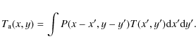
We use a correction algorithm developed by Kalberla et al. (1980a). Antenna
temperatures ![]() observed by radio telescopes can be approximated in
Cartesian coordinates as a convolution of the true temperature distribution
T on the sky with the beam pattern P of the antenna
observed by radio telescopes can be approximated in
Cartesian coordinates as a convolution of the true temperature distribution
T on the sky with the beam pattern P of the antenna
|
(1) |
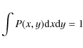
This is an approximation, but is sufficient to demonstrate the basics. In general,
For the pattern P of the antenna we use the normalization
|
(2) |
in addition, we split the pattern into the main beam area (MB) and the stray-pattern (SP)
| |
= | ||
| (3) |
Defining the main beam efficiency
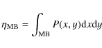
|
(4) |
we may rewrite Eq. (3) as
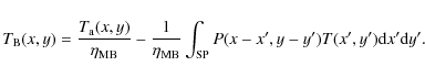
Replacing
![\begin{figure}
\par\includegraphics[angle=-90,width=5cm]{13979fig1a.ps} \include...
...979fig1c.ps} \includegraphics[angle=-90,width=6.cm]{13979fig1d.ps}
\end{figure}](/articles/aa/full_html/2010/13/aa13979-09/img38.png)
|
Figure 1:
Feed configuration for the receiver (top) and antenna patterns
within a radius of 6 |
| Open with DEXTER | |
2.2 The correction algorithm
The numerical correction algorithm is based on Kalberla et al. (1980a). It was
originally developed for the Effelsberg 100-m telescope, with some
improvements it was then applied to the LAB survey (Kalberla et al. 2005). We
modified this procedure for use with multi-beam systems, allowing individual
corrections for each of the beams. Due to the rotation of the offset receivers
with respect to the telescope structure, we take into account the variation of
each receiver's beam pattern on the sky with time. To improve the accuracy of
the calculations we also changed the convolution algorithm for the inner part
of the antenna response pattern (within 6![]() of the main beam). From the
LAB survey, a new and more accurate input sky for the convolution
(Eq. (5)) was generated.
of the main beam). From the
LAB survey, a new and more accurate input sky for the convolution
(Eq. (5)) was generated.
2.3 The multi-beam antenna pattern - near sidelobes
To solve Eq. (5) it is necessary to know the complete antenna response P for each of the 13 beams of the Parkes multi-feed system. In practice there are severe limitations in measuring the sidelobes to the required accuracy. We have therefore chosen to model the sidelobes. In general, the far-field pattern of an antenna is the autocorrelation of the aperture plane distribution. Using the measured feed response pattern and the telescope geometry, including shadowing caused by the focus cabin and the feed support legs, we derive the complex aperture distribution function for each feed. The pattern can then be calculated by Fourier transformation.
For the 13 beams we distinguished three characteristic cases, the central beam
and one feed from the inner and outer ring of feeds (Fig. 1
top). The feed horns are equipped with two pairs of orthogonal-linear probes,
which, while in parallactic tracking, rotate relative to the feed support
legs. In turn the complex aperture distribution function changes with time. We
approximate this rotation with an accuracy of
![]() .
The fact that the
three feed support legs cause a global six-fold symmetry for the antenna
pattern simplifies the situation considerably. We need only to calculate 5
individual patterns for each of the rings with radial feed offsets of
29
.
The fact that the
three feed support legs cause a global six-fold symmetry for the antenna
pattern simplifies the situation considerably. We need only to calculate 5
individual patterns for each of the rings with radial feed offsets of
29
![]() 1 and 50
1 and 50
![]() 8, respectively.
8, respectively.
Figure 1 shows the feed configuration for the multibeam
system![]() and displays the antenna response pattern within a radius of 6
and displays the antenna response pattern within a radius of 6![]() for feeds
1, 2, and 8. We see characteristic changes due to the beam displacements. The
main beam develops a coma lobe that increases in strength with feed
offset. Sidelobe structures become asymmetric and have a more pronounced
ringing with increasing feed offset. An important feature of the multi-feed
system is that the azimuthal asymmetries in the antenna pattern due to the
feed offsets decrease on average with increasing distance from the main
beam. Extrapolating this property to far sidelobes, offset from the main beam
by tens of degrees, implies that differences between individual feeds should
vanish. Indeed we verified this behavior as described in Sect. 2.4.
for feeds
1, 2, and 8. We see characteristic changes due to the beam displacements. The
main beam develops a coma lobe that increases in strength with feed
offset. Sidelobe structures become asymmetric and have a more pronounced
ringing with increasing feed offset. An important feature of the multi-feed
system is that the azimuthal asymmetries in the antenna pattern due to the
feed offsets decrease on average with increasing distance from the main
beam. Extrapolating this property to far sidelobes, offset from the main beam
by tens of degrees, implies that differences between individual feeds should
vanish. Indeed we verified this behavior as described in Sect. 2.4.
In the correction algorithm it is not necessary to use a pattern with all the
details shown in Fig. 1 as the LAB data were measured on a
grid of only
![]() .
We have therefore modeled the inner
6
.
We have therefore modeled the inner
6
![]() 0 of the antenna patterns on a grid containing 468 cells in cylindrical
coordinates. The cells have an azimuthal extent of 10
0 of the antenna patterns on a grid containing 468 cells in cylindrical
coordinates. The cells have an azimuthal extent of 10![]() and a radial extent
of 0
and a radial extent
of 0
![]() 2 out to 2
2 out to 2
![]() 2 from the main beam, a radial extent of 0
2 from the main beam, a radial extent of 0
![]() 3 out to
2
3 out to
2
![]() 5, and of 0
5, and of 0
![]() 5 thereafter.
5 thereafter.
2.4 The far sidelobes
The far sidelobes arise predominantly by reflections from the feed support legs, causing the so-called stray-cones, and at the rim of the telescope, the spillover. The location of these structures on the sky was determined from the telescope geometry and verified by numerous tests made with a transmitter. The sidelobe levels from the spillover lobes were estimated from the edge taper of the receiver feed. For the stray-cones we used estimates from the the aperture blocking by the feed legs. These estimates were also based on sidelobe levels found previously for the telescopes at Effelsberg, Dwingeloo and Villa Elisa (Kalberla et al. 2005; Hartmann et al. 1996; Kalberla et al. 1980a; Bajaja et al. 2005). The far sidelobe components were adjusted individually in a way similar to that described by Kalberla et al. (2005), searching for a consistent solution of Eq. (5).
2.5 Ground reflections
Sidelobes that touch the ground receive broad-band thermal noise, but to first order no line radiation is expected. However, depending on the ground cover, reflections may happen. While scrub acts as an absorber, low grass and soil can reflect 21-cm line radiation. We determine this contribution by surveying the ground around the telescope, and then using ray-tracing methods to estimate the effective sidelobe response. We used an albedo of 0.2.
3 Removal of instrumental baselines
3.1 Preliminary considerations
In many cases, stray-radiation produces extended profile wings that mistakenly may be interpreted as instrumental baseline structure. A correction for stray-radiation could cause negative intensities if applied after the baseline correction. It is therefore essential to apply baseline corrections only after the stray-radiation is eliminated. For this reason we had to deviate from the processing described in Naomi2009; for the first data release no correction for stray-radiation was applied. We used Livedata as described in their Sect. 2.3 for the bandpass correction, but without the post processing for baselines according to Sect. 2.3.3 in Naomi2009. The algorithm described below is in lieu of the post-processing described in Naomi2009.
After scaling the reduced data to antenna temperatures corrected for atmospheric absorption (Sect. 4) the stray-radiation was subtracted and afterwards the instrumental baseline was corrected. Flags set by Livedata or our own software to indicate the presence of RFI were taken into account, and affected channels were disregarded for all of the baseline fits described below.
3.2 The algorithm
For each spectrum of the stray-radiation-corrected GASS database we used the
LAB survey for an initial estimate of the velocity extent of the expected H I
emission. After smoothing the interpolated LAB profile to an effective
resolution of
![]() km s-1, we used velocities where
km s-1, we used velocities where
![]() K as the range for an initial fit of the instrumental GASS baseline. In
addition we folded the LAB profile in frequency to mimic the second spectrum
used by Livedata to determine the instrumental bandpass
[][Fig. 3]Naomi2009. Flags were transferred accordingly.
K as the range for an initial fit of the instrumental GASS baseline. In
addition we folded the LAB profile in frequency to mimic the second spectrum
used by Livedata to determine the instrumental bandpass
[][Fig. 3]Naomi2009. Flags were transferred accordingly.
GASS spectra from both polarizations were averaged and smoothed to
![]() km s-1 for each of the individual 5 s dumps. Using the initial
estimate for the emission-free part of the profile we determined the
instrumental baseline by fitting a 9th order polynomial. Any channel
with signal exceeding four times the rms noise over the fitted region was
considered to contain possible H I emission and was then excluded from the
baseline region. The baseline fit was repeated with an 11th order
polynomial, again searching for potential emission that needed to be excluded
from the fit. As a measure of the fit quality we determined the residual rms
scatter within the baseline region. For a few percent of the data we found
that a 9th order polynomial provided a better fit. Accordingly we used
this fit. Finally we took into account that weak profile wings with
intensities below the automatic
km s-1 for each of the individual 5 s dumps. Using the initial
estimate for the emission-free part of the profile we determined the
instrumental baseline by fitting a 9th order polynomial. Any channel
with signal exceeding four times the rms noise over the fitted region was
considered to contain possible H I emission and was then excluded from the
baseline region. The baseline fit was repeated with an 11th order
polynomial, again searching for potential emission that needed to be excluded
from the fit. As a measure of the fit quality we determined the residual rms
scatter within the baseline region. For a few percent of the data we found
that a 9th order polynomial provided a better fit. Accordingly we used
this fit. Finally we took into account that weak profile wings with
intensities below the automatic ![]() cut-off level could affect the fit
parameters. To avoid such a bias we excluded 6 more channels on each side of
the H I emission from the baseline region that was fitted.
cut-off level could affect the fit
parameters. To avoid such a bias we excluded 6 more channels on each side of
the H I emission from the baseline region that was fitted.
After these initial steps we considered both spectra for each polarization individually. The spectra were smoothed and fitted with the parameters determined previously to find out whether some more features needed to be excluded from the baseline region. After that the final baseline fit was applied to the original observations.
The algorithm and the parameters described above were tested and optimized by varying the polynomial order and trying other functional forms. We particularly tried to avoid high order polynomials. As described in Naomi2009, the average quotient spectrum for each of the scans (visible as patches in Fig. 9, bottom) was fitted with a 15th order polynomial. Figure 3 of Naomi2009 demonstrates that emission features are not affected by this fit. After this global bandpass fit there remain some time dependent fluctuations that need to be corrected independently for each spectrum with 5 s integration time. A first guess would be that a similar polynomial is needed to get rid of such fluctuations. This is fortunately not the case. In the initial Livedata reduction for the first data release a 10th order fit for post-processing of individual spectra was sufficient. Our results confirm this finding with minor modifications for our procedure. We tested lower order polynomials. These led for many regions to obvious baseline defects. We found spurious features in emission free regions that could only be avoided by allowing higher orders.
Assuming that some parts of the residual baseline ripples could be caused by standing waves, we also tested sine wave fits in addition to polynomials. Sinusoid solutions were found to be insignificant and were discarded. We carefully checked whether errors in the LAB data might affect the GASS baseline correction, but the iterative refinements that were applied successfully avoided any biases. We tested also whether the high order polynomial fits might have affected weak emission features. We found no indications for such problems. In particular the RFI feature observed in March 2006, appearing similar to a HVC (Sect. 5.5), remained unaffected by the fit. Also testing whether profile wings in data that remained uncorrected for stray-radiation could be removed by baseline fitting did not indicate an unwanted overcorrection by the baseline fit (see Sect. 7).
Some residual systematical baseline problems remain in a few regions, on average typically at a level of ![]() 40 mK but occasionally up to 100 mK. This is close to the rms uncertainties of
40 mK but occasionally up to 100 mK. This is close to the rms uncertainties of ![]() 60 mK for individual maps as discussed in Sect. 7.
We were unable to identify the reason for such systematic baseline
errors. They may be caused by RFI or bad fits but also by uncertainties
in the stray-radiation correction.
60 mK for individual maps as discussed in Sect. 7.
We were unable to identify the reason for such systematic baseline
errors. They may be caused by RFI or bad fits but also by uncertainties
in the stray-radiation correction.
![\begin{figure}
\par\mbox{\includegraphics[angle=-90,width=9cm]{13979fig2a.eps} \includegraphics[angle=-90,width=9cm]{13979fig2b.eps} }
\end{figure}](/articles/aa/full_html/2010/13/aa13979-09/img46.png)
|
Figure 2: Left: gain factors applied to the initial calibration (blue stars and purple squares) and cross check after the final data reduction (red plus signs and green X's). Right: rms scatter in gain calibration for individual feeds, before and after correction for stray-radiation (same symbols as in left panel). |
| Open with DEXTER | |
4 Calibration
An accurate correction for stray-radiation demands a careful
calibration. Errors in the antenna temperature scale cause a mismatch with the
stray-radiation correction term in Eq. (5). The sidelobe
response is frequency dependent; calibration errors, therefore, cause not only
an increased scale error but also affect the profile shape. We used regular
observations at the standard positions S8, S9, and S6 (Williams 1973) and
determined average calibration factors for each of the observing sessions. An
initial temporary calibration was determined from uncorrected data
Naomi2009. After correcting the data for stray-radiation we
redetermined the ![]() calibration factors and applied these new factors for
the following calculations.
calibration factors and applied these new factors for
the following calculations.
Table 2 lists the final calibration data; the brightness temperature scale is matched to a common temperature scale first established by Williams (1973). The brightness temperature for most of the major surveys are matched through this reference; this includes the Hat Creek surveys (Heiles & Habing 1974; Weaver & Williams 1973), the Leiden-Green Bank survey (Burton 1985), southern sky surveys by Kerr et al. (1981), the Bell Labs survey (Stark et al. 1992), the LAB survey, and Effelsberg and Arecibo data (Winkel et al. 2010; Peek & Heiles 2008).
A few calibration regions have been mapped by Kalberla et al. (1982). They
calculated the beam response in detail and provided also calibration factors
as a function of the beam shape. We use factors appropriate for a 14.4![]() beam.
beam.
The easiest way to determine the calibration factors is to use peak temperatures, but line integrals over a limited velocity range are more accurate (Williams 1973) and we preferred this method. Please note that velocities listed in Table 2 are integration limits while velocities given by Williams (1973) are center velocities for the edge channels (see Kalberla et al. 1982). Figure 2 (left) compares overall gain factors applied to the initial calibrations (blue) with those after completing the final corrections (red and green). The overall calibration uncertainties (right) for most of the feeds could be reduced to typically 1.7%. Only two receivers were less stable with an rms scatter of 3% and 3.5%. The uncertainties are of statistical nature. Combining observations with several beams at different seasons we expect average temperature scale uncertainties well below 1% in the final data. We note that interference can cause a loss of calibration in some spectra that would be difficult to detect as it would appear as a scale factor over an entire spectrum. We believe that this effect is small in the overall survey but may be present in some final spectra.
Table 2:
![]() calibration positions and parameters.
calibration positions and parameters.
![\begin{figure}
\par\mbox{\includegraphics[angle=-90,width=9.cm]{13979fig3a.eps} \includegraphics[angle=-90,width=9.cm]{13979fig3b.eps} }
\end{figure}](/articles/aa/full_html/2010/13/aa13979-09/img47.png)
|
Figure 3: Typical example for extended interference patterns that were flagged by Livedata in the first stage of the data reduction. Left: as observed, right: after RFI removal using LAB data as described in Sect. 5.1. The intensity scale is linear for -0.2 < T < 0.5 K. Some weak structures remain but are mostly at |T| < 40 mK. |
| Open with DEXTER | |
5 RFI mitigation
5.1 Replacement of data flagged by Livedata
Narrow-line interference was flagged during the basic data reduction with Livedata [][Sect. 2.3.2]Naomi2009. Most of this type of RFI
occurs at a fixed topocentric frequency, so as the telescope scans across the
sky the RFI moves in successive channels in the LSRK frame. We use the
kinematical (radio) standard of rest definition with a velocity of 20 km s-1 in
direction Ra, Dec = [270![]() , +30
, +30![]() ]
(epoch 1900.0). Most of the features are
observed to stretch over large angular distances and affect fields that have
been observed independently at different seasons (Fig. 3). This
behavior implies that the RFI remained approximately constant for long periods
in time, affecting most of the data.
]
(epoch 1900.0). Most of the features are
observed to stretch over large angular distances and affect fields that have
been observed independently at different seasons (Fig. 3). This
behavior implies that the RFI remained approximately constant for long periods
in time, affecting most of the data.
Profiles with more then 30 flagged channels were completely discarded during imaging; for less serious contaminations the flagged data were replaced. After correcting profiles for stray-radiation and instrumental baseline, we interpolated LAB survey data to replace the flagged channels. Alternatively we have tried to replace data by interpolating the GASS spectra using the nearest ten good data points. Using LAB data resulted in all cases in much cleaner maps. Still, some weak stripy features remain that appear to move across the sky in successive velocity channels but mostly these artifacts remain within the noise (Fig. 3). About 0.1% of all data have been flagged by Livedata and were replaced by interpolated data in this first step. We kept the Livedata flags to avoid such interpolated data getting propagated by the RFI mitigation described in the following sections.
5.2 Median filter RFI rejection
Even after removal of the channels flagged in the initial data reduction, numerous instances of RFI remain in the data. Some appear as point sources, but the most obvious show ``footprints'' of the 13-beam system that move on the sky in scanning direction (Fig. 4). As before, the motion in successive velocity channels is caused by changing LSR projections of the fixed Topocentric RFI frequencies. Features of this kind were found previously in the HIPASS and are described in detail by Barnes et al. (2001, Fig. 7). For the first data release the remaining RFI was removed by median gridding when calculating FITS images [][Sect. 2.3.5]Naomi2009.
![\begin{figure}
\par\mbox{\includegraphics[angle=-90,width=9.cm]{13979fig4a.eps} \includegraphics[angle=-90,width=9.cm]{13979fig4b.eps} }
\end{figure}](/articles/aa/full_html/2010/13/aa13979-09/img48.png)
|
Figure 4:
HI emission at
|
| Open with DEXTER | |
Here we follow a different strategy, taking advantage of the fact that in GASS
typically 40 individual spectra contribute to the final data in every
resolution element. First, for any observed position in the sky we selected
all observed profiles within an angle ![]() of typically a few
arc-minutes. From these data we calculate the mean for each channel, the
corresponding standard deviation, and the median, disregarding data flagged
either by Livedata or our own post-processing. The average rms noise
level
of typically a few
arc-minutes. From these data we calculate the mean for each channel, the
corresponding standard deviation, and the median, disregarding data flagged
either by Livedata or our own post-processing. The average rms noise
level
![]() and its one sigma deviation
and its one sigma deviation
![]() from the average was determined for the low level emission part of the profile
(
from the average was determined for the low level emission part of the profile
(
![]() K).
K).
We have two tests for RFI. In the first, channels with rms deviations
![]() were considered as highly suspicious for RFI
contamination and investigated in more detail. We use as a second indication
of RFI circumstances where the mean and median differ from each other by more
than one standard deviation.
were considered as highly suspicious for RFI
contamination and investigated in more detail. We use as a second indication
of RFI circumstances where the mean and median differ from each other by more
than one standard deviation.
To eliminate outliers for the channels that were selected in both of the two tests we determined if individually observed brightness temperatures deviate from the median by more than two times the standard deviation. In the case of a purely random distribution this would exclude 5% of the good data, and we consider this an acceptable cost to eliminate true RFI. We flag outliers and repeat, calculating new mean and median estimators and once more excluding any outliers.
Our two sigma limit may be compared with the more rigorous method for the
elimination of suspect data proposed by Peirce (1852) which is based on
probability theory. Accordingly a rejection of a data point that deviates from
the mean at a two sigma level is justified if there are 13 independent
observed data values. For
![]() (see below) we have on average
40 individual profiles and a two sigma limit is appropriate if about 10% of
the data are suspect. This condition is valid for many cases but we find also
situations where 20% of the measurements are outliers. In this case a cutoff
at
(see below) we have on average
40 individual profiles and a two sigma limit is appropriate if about 10% of
the data are suspect. This condition is valid for many cases but we find also
situations where 20% of the measurements are outliers. In this case a cutoff
at
![]() would be more appropriate according to
Peirce (1852). We deviate from Peirce's criterion in two ways; to
simplify the calculations we use a fixed
would be more appropriate according to
Peirce (1852). We deviate from Peirce's criterion in two ways; to
simplify the calculations we use a fixed
![]() cutoff and we
define outliers by their deviations from the median and not, as originally
proposed by Peirce, from the mean. The latter is essential since outliers
caused by RFI can be found at ten to hundred times the standard deviation, a
circumstance that was not considered by Peirce; in such cases the mean is
usually seriously affected.
cutoff and we
define outliers by their deviations from the median and not, as originally
proposed by Peirce, from the mean. The latter is essential since outliers
caused by RFI can be found at ten to hundred times the standard deviation, a
circumstance that was not considered by Peirce; in such cases the mean is
usually seriously affected.
To replace values outside the two sigma range, the best available estimate is
the median value scaled by the proper beam weighting function, for details we
refer to the extended discussion by Barnes et al. (2001, Sect. 4.2.2). We
replace the previously selected data points by the weighted median and set a
flag to distinguish medians from observed values. A fraction ![]()
![]() of the data is affected by RFI and replaced by the weighted median.
of the data is affected by RFI and replaced by the weighted median.
One of the criteria that we used to detect RFI was the fact that mean and median should not differ by more than one standard deviation. We applied this criterion also to test whether the median estimator is consistent with the mean of all data after exclusion of the outliers. Both methods were found to produce nearly identical results. An example of RFI in scanning direction and the result after application of our median filer is given in Fig. 4.
Figure 5 shows spectral details for one position in this
field. Displayed are the mean (red), the rms scatter (green), and the median
(blue) derived for all profiles that are closer than
![]() to
the position
to
the position
![]() ,
,
![]() .
Data in the left plot suffer from
strong interference at
.
Data in the left plot suffer from
strong interference at
![]() km s-1,
km s-1,
![]() km s-1, and at
km s-1, and at
![]() km s-1. Only a part of the data
was flagged by Livedata and replaced by values from the LAB. Despite all
defects the median (blue) is essentially unaffected by RFI. The data after RFI
elimination are shown in the plot at the right side. Profiles for mean and
median are within the noise identical, the rms is close to the expected value
of 0.4 K and shows no strong enhancements. We find some fluctuations close to
the line emission at
km s-1. Only a part of the data
was flagged by Livedata and replaced by values from the LAB. Despite all
defects the median (blue) is essentially unaffected by RFI. The data after RFI
elimination are shown in the plot at the right side. Profiles for mean and
median are within the noise identical, the rms is close to the expected value
of 0.4 K and shows no strong enhancements. We find some fluctuations close to
the line emission at
![]() km s-1. This may have been caused by
genuine fluctuations in the H I line emission. To avoid a possible
degradation of such fluctuations no automatic RFI cleaning was applied for
km s-1. This may have been caused by
genuine fluctuations in the H I line emission. To avoid a possible
degradation of such fluctuations no automatic RFI cleaning was applied for
![]() K. These two plots demonstrate how greatly the rms is affected by
RFI, and how deviations between median and mean are obvious. Our RFI filter is
triggered by such deviations.
K. These two plots demonstrate how greatly the rms is affected by
RFI, and how deviations between median and mean are obvious. Our RFI filter is
triggered by such deviations.
5.3 The beam-specific parameter 
A critical parameter for RFI filtering is the radius ![]() for a
comparison of the data at adjacent positions. A large value provides a large
statistical sample but at the same time point sources or steep gradients in
the brightness distribution may be affected by the filter. We found in tests
that
for a
comparison of the data at adjacent positions. A large value provides a large
statistical sample but at the same time point sources or steep gradients in
the brightness distribution may be affected by the filter. We found in tests
that
![]() is sufficiently robust. Tests with H I
point-sources have shown that larger values could degrade the source
distribution. Our result is in excellent agreement with
Barnes et al. (2001), and our median estimator is
identical with the parameter
is sufficiently robust. Tests with H I
point-sources have shown that larger values could degrade the source
distribution. Our result is in excellent agreement with
Barnes et al. (2001), and our median estimator is
identical with the parameter
![]() that was used for HIPASS.
that was used for HIPASS.
![\begin{figure}
\par\mbox{ \includegraphics[angle=-90,width=9.cm]{13979fig5a.eps} \includegraphics[angle=-90,width=9.cm]{13979fig5b.eps} }
\end{figure}](/articles/aa/full_html/2010/13/aa13979-09/img65.png)
|
Figure 5:
Data at the position
|
| Open with DEXTER | |
5.4 RFI in emission line regions
RFI that falls in channels containing H I emission was usually removed successfully by the above procedure, except in regions with strong spectral gradients. Examples of such critical cases are positions with strong absorption lines. Sources with a continuum flux exceeding 200 mJy were excluded from RFI rejection.
To avoid any possible degradation of the signal due to an automatic RFI
filtering, the median filters described in Sect. 5.2 were restricted
to data with low brightness temperatures. We used a limit of
![]() K. The remaining data were checked visually. Only a few cases showed some
residual RFI. For these we increased the filter limits such that only channels
with sufficient large rms deviation
K. The remaining data were checked visually. Only a few cases showed some
residual RFI. For these we increased the filter limits such that only channels
with sufficient large rms deviation
![]() were affected. We
verified that the remaining data were unaffected by the median filter. As a
general rule we tried to avoid as far as possible any modification of the H I
emission lines through the RFI filtering process. This implies, however, that
some RFI may remain undetected and be present in the final data.
were affected. We
verified that the remaining data were unaffected by the median filter. As a
general rule we tried to avoid as far as possible any modification of the H I
emission lines through the RFI filtering process. This implies, however, that
some RFI may remain undetected and be present in the final data.
Some of the spectra were affected so severely by RFI that they needed to be removed completely. We eliminated all profiles whose mean rms within the baseline region exceeded the average noise level at its position by a factor of three. About 0.3% of the observed profiles were rejected for this reason.
5.5 RFI in March 2006
For a short period between 18 and 21 March 2006 observations were degraded by broadband RFI with quite different characteristics than any of the narrow band RFI described above. The weak spurious lines had approximately Gaussian shapes with center velocities in the range 270 to 310 km s-1 and velocity dispersions of about 15 km s-1. None of the RFI rejection methods described above applied to this case. These spurious lines were identified by fitting Gaussians; all affected channels were then flagged. Baseline corrections were repeated, finally all flagged data were replaced by medians as described before. This way we recovered data that were discarded in the first data release.
5.6 Removal of bandpass ghosts
To maximize sensitivity and recover all the extended H I emission, the GASS
was made using in-band frequency-switching with an offset of 3.125 MHz
corresponding to 660 km s-1. The Livedata bandpass correction causes for
every real emission line feature an associated, spurious, negative image
(``ghost'') in the other band, displaced by ![]() km s-1. Most of these
negative images fall outside the velocity coverage of the survey but high
velocity clouds (HVCs) with emission lines at
km s-1. Most of these
negative images fall outside the velocity coverage of the survey but high
velocity clouds (HVCs) with emission lines at
![]() km s-1 cause ghosts. In particular, the Magellanic System causes a strong and
extended bandpass ghost at negative velocities.
km s-1 cause ghosts. In particular, the Magellanic System causes a strong and
extended bandpass ghost at negative velocities.
As Fig. 3 of Naomi2009 shows, ghosts appear only in one of the
two IFs; the other band is unaffected. It is possible to produce maps without
ghost features if one uses only one IF for
![]() km s-1. A
second possibility is to flag ghosts and eliminate them with a treatment
analogous to one of the the RFI mitigation strategies discussed above.
Accordingly the ghosts were replaced by medians determined from the alternate
ghost-free IF band. Such maps have the advantage that they provide a better
sensitivity for most of the field but remaining biases can not be excluded.
We determined for both bands all HVC emission features with
km s-1. A
second possibility is to flag ghosts and eliminate them with a treatment
analogous to one of the the RFI mitigation strategies discussed above.
Accordingly the ghosts were replaced by medians determined from the alternate
ghost-free IF band. Such maps have the advantage that they provide a better
sensitivity for most of the field but remaining biases can not be excluded.
We determined for both bands all HVC emission features with
![]() km s-1 and
km s-1 and
![]() K (corresponding to
K (corresponding to
![]() for
for
![]() )
and flagged ghosts in the other band. These features
were treated analogously to the broadband RFI discussed in the previous
section.
)
and flagged ghosts in the other band. These features
were treated analogously to the broadband RFI discussed in the previous
section.
6 Imaging
For HIPASS, as well as for the first data release of the GASS, imaging was
performed by Gridzilla using weighted median estimation which is robust
against RFI and other artifacts. For the second data release, we use separate
and independent procedures for RFI rejection and imaging. As described in the
previous section, our median filter is largely consistent with the HIPASS
median filter algorithm for a radius
![]() .
However, the major
difference is that we apply this filter only to individual channels if two
conditions apply: 1) an exceedingly large scatter is observed with a 3 times
larger dispersion than the mean dispersion caused by thermal noise and 2) mean
and median differ by more than one standard deviation. Only data that deviate
from the median by
.
However, the major
difference is that we apply this filter only to individual channels if two
conditions apply: 1) an exceedingly large scatter is observed with a 3 times
larger dispersion than the mean dispersion caused by thermal noise and 2) mean
and median differ by more than one standard deviation. Only data that deviate
from the median by
![]() are replaced by
the median estimate.
are replaced by
the median estimate.
![\begin{figure}
\par\includegraphics[angle=-90,width=8cm]{13979fig6.eps}
\end{figure}](/articles/aa/full_html/2010/13/aa13979-09/img73.png)
|
Figure 6:
Effective FWHM resolution W of GASS images as a function of the
user-definable Gaussian interpolation kernel |
| Open with DEXTER | |
For the data release described here the gridding was performed using a
two-dimensional Gaussian with a user-definable dispersion. For computational
reasons we disregard data outside a three sigma cutoff radius. The
interpolated value for that pixel is the weighted mean over all available
input data. Except for the irregular distribution on the sky of the input
data, this interpolation is equivalent to a linear convolution of the observed
brightness temperature distribution with the kernel function of the
gridder. The resulting effective beam is approximately Gaussian. For a source
width ![]() ,
an effective average telescope beam width of
,
an effective average telescope beam width of ![]() ,
and a width
,
and a width
![]() of the user defined kernel we expect a resulting FWHM width
of the user defined kernel we expect a resulting FWHM width
|
(6) |
We tested this relation by generating a series of images of the ultra-compact high-velocity cloud HVC289+33+251 (Brüns & Westmeier 2004; Putman et al. 2002). We used a grid spacing of
Next we deconvolve the observed and fitted FWHM width
![]() of the image
for the finite width
of the image
for the finite width
![]() of the source,
of the source,
![]() .
In Fig. 6 we plot W as a function of the convolving
kernel width
.
In Fig. 6 we plot W as a function of the convolving
kernel width ![]() .
To a good approximation we find for
.
To a good approximation we find for
![]() the simple relation
the simple relation
![]() .
For a kernel
.
For a kernel
![]() we obtain
we obtain
![]() ,
identical with the resolution of the
images calculated from weighted median estimators as presented in
Naomi2009.
,
identical with the resolution of the
images calculated from weighted median estimators as presented in
Naomi2009.
![\begin{figure}
\par\includegraphics[angle=-90,width=8cm]{13979fig7.eps}
\end{figure}](/articles/aa/full_html/2010/13/aa13979-09/img89.png)
|
Figure 7: Effective rms uncertainties of GASS channel maps with 1 km s-1 velocity resolution as a function of the user-definable Gaussian interpolation kernel. Crosses indicate fitted values determined at high Galactic latitudes, the solid black line represents upper limits of the noise, valid for most of the positions in the Galactic plane. For comparison we show the effective noise at high latitudes obtained by median gridding and by Bessel interpolation (horizontal lines). |
| Open with DEXTER | |
![\begin{figure}
\par\includegraphics[angle=-90,width=14.5cm]{13979fig8a.eps}
\i...
...8b.eps}
\includegraphics[angle=-90,width=14.5cm]{13979fig8c.eps}
\end{figure}](/articles/aa/full_html/2010/13/aa13979-09/img90.png)
|
Figure 8:
HI emission at
|
| Open with DEXTER | |
![\begin{figure}
\par\includegraphics[angle=-90,width=14.5cm]{13979fig9a.eps}
\includegraphics[angle=-90,width=14.5cm]{13979fig9b.eps}
\end{figure}](/articles/aa/full_html/2010/13/aa13979-09/img91.png)
|
Figure 9:
Top: stray-radiation contribution removed from the GASS at
|
| Open with DEXTER | |
The noise level of the output map depends on the user defined smoothing
kernel. We measured the noise in the same FITS cubes that we used to fit
beamwidths, at a velocity of 240 km s-1 where neither H I emission nor RFI is
visible. Figure 7 gives the results. The noise strongly depends
on the smoothing kernel; for
![]() we obtain an rms brightness
temperature noise of 57 mK, comparable to the results in
Naomi2009. The corresponding effective resolution is
we obtain an rms brightness
temperature noise of 57 mK, comparable to the results in
Naomi2009. The corresponding effective resolution is
![]() .
.
The noise level depends on the strength of the line emission. Within the
Galactic plane for
![]() we find a typical increase by a factor of
1.75. This approximate upper limit is plotted in Fig. 7. For a
detailed map of the uncertainties we refer to the bottom map in
Fig. 9. In this case
we find a typical increase by a factor of
1.75. This approximate upper limit is plotted in Fig. 7. For a
detailed map of the uncertainties we refer to the bottom map in
Fig. 9. In this case
![]() was chosen, resulting in a
typical noise level of 35 mK. It is obvious that the noise in the final maps
is affected by RFI mitigation and observational setup. Overlap regions for the
raster chosen are clearly visible.
was chosen, resulting in a
typical noise level of 35 mK. It is obvious that the noise in the final maps
is affected by RFI mitigation and observational setup. Overlap regions for the
raster chosen are clearly visible.
We tested also the optimal gridding of single dish on-the-fly observations as
proposed by Mangum et al. (2007) with the function
J1 is the Bessel function, a = 1.55, and b = 2.52 for a grid of 1/3 FWHM. This is the default for the AIPS task SDGRD (Greisen 1998). The resulting resolution and noise are plotted as horizontal lines in Figs. 6 and 7. Both median gridding according to Naomi2009 and optimal Bessel filtering are consistent with a Gaussian gridding for a kernel of
7 Quality of the data
To aid in the discussion of this release of the GASS data we have chosen a
channel map at
![]() km s-1 (Fig. 8). At this
velocity stray-radiation effects are strong and residual problems easily
visible. In the top panel of Fig. 8, we show a map that was
generated without a stray-radiation correction but with the instrumental
baselines removed as described in Sect. 3. In the middle panel,
we plot the map from the final GASS database, corrected for stray-radiation
and instrumental baseline. We have chosen a FWHM kernel
km s-1 (Fig. 8). At this
velocity stray-radiation effects are strong and residual problems easily
visible. In the top panel of Fig. 8, we show a map that was
generated without a stray-radiation correction but with the instrumental
baselines removed as described in Sect. 3. In the middle panel,
we plot the map from the final GASS database, corrected for stray-radiation
and instrumental baseline. We have chosen a FWHM kernel
![]() ,
resulting in rms uncertainties of
,
resulting in rms uncertainties of ![]() 35 mK at intermediate Galactic
latitudes. In the bottom panel of Fig. 8, we show the same
channel from the LAB database for comparison. Figure 9 (top)
contains the stray-radiation contribution removed from the middle map in
Fig. 8.
35 mK at intermediate Galactic
latitudes. In the bottom panel of Fig. 8, we show the same
channel from the LAB database for comparison. Figure 9 (top)
contains the stray-radiation contribution removed from the middle map in
Fig. 8.
The bottom panel of Fig. 9 displays a compilation of the residual
![]() rms uncertainties for a FITS cube generated with FWHM kernel
rms uncertainties for a FITS cube generated with FWHM kernel
![]() These uncertainties depend on the integration time and on the system
noise. Enhanced noise is caused by low elevation observations, by continuum
emission from the Galactic plane, or by RFI mitigation (rejecting data).
These uncertainties depend on the integration time and on the system
noise. Enhanced noise is caused by low elevation observations, by continuum
emission from the Galactic plane, or by RFI mitigation (rejecting data).
The final GASS map, Fig. 8 middle, shows no obvious evidence of
residual stray-radiation problems. Time dependence of stray-radiation would
cause a correlation with the observational grid that is easily visible in
Fig. 9 (bottom). Such residual problems can be seen in the LAB
channel map (Fig. 8 bottom). Individual blocks, corresponding to
a grid of
![]() positions, show up at latitudes of
positions, show up at latitudes of
![]() ,
a
problem already mentioned by Kalberla et al. (2005). Similar block structures
existed also in the first version of the Leiden/Dwingeloo Survey
(Hartmann et al. 1996; Hartmann & Burton 1997) but could be removed by an improved
stray-radiation correction in the second data release of the LAB
(Kalberla et al. 2005). Time variability is caused predominantly by a seasonal
variation of the stray-radiation and needs to be minimized by the correction
(Kalberla et al. 1980b,a). The final GASS database is much less
affected by residual instrumental problems than the LAB survey. This implies
in particular that there was no error propagation from the LAB to the GASS. We
conclude that our corrections successfully removed most of the sidelobe
influences, remaining systematical errors are probably below 1%. The
performance of the survey is equivalent to observations with a telescope
having
,
a
problem already mentioned by Kalberla et al. (2005). Similar block structures
existed also in the first version of the Leiden/Dwingeloo Survey
(Hartmann et al. 1996; Hartmann & Burton 1997) but could be removed by an improved
stray-radiation correction in the second data release of the LAB
(Kalberla et al. 2005). Time variability is caused predominantly by a seasonal
variation of the stray-radiation and needs to be minimized by the correction
(Kalberla et al. 1980b,a). The final GASS database is much less
affected by residual instrumental problems than the LAB survey. This implies
in particular that there was no error propagation from the LAB to the GASS. We
conclude that our corrections successfully removed most of the sidelobe
influences, remaining systematical errors are probably below 1%. The
performance of the survey is equivalent to observations with a telescope
having ![]() 99% main beam efficiency. Scale uncertainties, caused by gain
fluctuations, are also probably below 1% (Sect. 4).
99% main beam efficiency. Scale uncertainties, caused by gain
fluctuations, are also probably below 1% (Sect. 4).
The top panel of Fig. 8, shows that stray-radiation can not be removed with only our baseline correction algorithm as most of the stray-radiation remains in the map. This also demonstrates that our baselining algorithm is safe in the sense that it does not noticeably affect extended profile wings.
We searched for remaining systematical uncertainties in the instrumental baseline. Some residual uncertainties caused by RFI are visible in individual channel maps. In most cases such defects remain on average below 40 mK but there are a few more serious cases. In critical cases we recommend comparing GASS data with the LAB database. Also a comparison of the cleaned database with the dirty data, offered by the web interface, may be helpful.
8 Data products
Data from the first release are accessible at http://www.atnf.csiro.au/research/GASS/Data.html. We provide a web interface at http://www.astro.uni-bonn.de/hisurvey for the second release to retrieve spectra and column densities for individual positions or complete FITS cubes. The user can specify Galactic or Equatorial coordinates, the velocity range, and the FWHM of the smoothing kernel for the optimal resolution. Default values for the gridding are provided as well. Some restrictions to the sizes of the FITS cubes apply, and we currently provide maps only in Cartesian projection.
The user can check the data for residual contaminations by RFI or
stray-radiation by downloading FITS cubes with dirty data (corrected for
baseline and stray-radiation but no RFI filtering applied) or stray-radiation
corrections that were subtracted as described in Sect. 2. Data at high
velocities
![]() km s-1 can be generated alternatively from
both IFs or from single ``ghost-free'' IFs only (see Sect. 5.6). In
the latter case the rms noise for channels at velocities
km s-1 can be generated alternatively from
both IFs or from single ``ghost-free'' IFs only (see Sect. 5.6). In
the latter case the rms noise for channels at velocities
![]() km s-1 increases by a factor of
km s-1 increases by a factor of ![]() .
.
Despite all efforts some instrumental problems may still exist in the second data release. Our web based policy for the on-the-fly generation of FITS cubes allows appropriate corrections. We ask users of the GASS data to report problems. Information on updates of the database will be provided on the web page.
9 Summary
The Parkes Galactic All-Sky Survey (GASS) measured the H I emission in the
Southern sky with complete sampling at all declinations
![]() using the Parkes Radioe Telescope. The survey has an effective angular
resolution of
using the Parkes Radioe Telescope. The survey has an effective angular
resolution of
![]() at a velocity resolution of 1.0 km s-1, and the data
were obtained in a way that is sensitive to extended diffuse emission as well
as compact sources. The GASS database contains
at a velocity resolution of 1.0 km s-1, and the data
were obtained in a way that is sensitive to extended diffuse emission as well
as compact sources. The GASS database contains
![]() individual
spectra with 5 s integration time observed by on-the-fly mapping. The
first data release together with a detailed description of the survey goals
and techniques was given in Naomi2009. Here we focus on the post
processing to correct instrumental effects including stray-radiation, radio
frequency interference, and residual instrumental spectral baselines.
individual
spectra with 5 s integration time observed by on-the-fly mapping. The
first data release together with a detailed description of the survey goals
and techniques was given in Naomi2009. Here we focus on the post
processing to correct instrumental effects including stray-radiation, radio
frequency interference, and residual instrumental spectral baselines.
The GASS is the most sensitive, highest angular resolution survey of Galactic
H I emission ever made of the Southern sky. After correcting for instrumental
effects and RFI the GASS data are in excellent agreement with the LAB
survey. This is impressively demonstrated with Fig. 8. FITS data
cubes are available on request from http://www.astro.uni-bonn.de/hisurvey.
Our software allows a flexible generation of FITS datacubes with effective
resolutions
![]() (Fig. 6). The
corresponding rms noise fluctuations at high Galactic latitudes are in the
range
(Fig. 6). The
corresponding rms noise fluctuations at high Galactic latitudes are in the
range
![]() mK (Fig. 7). We provide clean
maps as the final product from our data processing but also maps without RFI
elimination. To allow estimates on possible residual stray-radiation effects
it is also possible to extract the corrections which were applied.
mK (Fig. 7). We provide clean
maps as the final product from our data processing but also maps without RFI
elimination. To allow estimates on possible residual stray-radiation effects
it is also possible to extract the corrections which were applied.
We thank Butler Burton for a very thorough refereeing of this paper with constructive criticism and many valuable suggestions. The GASS would have not been possible without support from the ATNF staff at Parkes and Sydney. We greatly acknowledge assistance in determining the propertiesof the antenna pattern from M. Kesteven, M. Price, J. Reynolds, and W. Wilson. P. Müller (MPIfR Bonn) provided software for baseline fitting. This project was supported by Deutsche Forschungsgemeinschaft, DFG grant KA1265/5-2. P.K. acknowledges also support during a productive stay in Sydney as a distinguished visitor of the ATNF. The Parkes Radio Telescope is part of the Australia Telescope which is funded by the Commonwealth of Australia for operation as a National Facility managed by CSIRO. D.J.P. acknowledges partial support for this project from NSF grant AST0104439 and from an international faculty development grant from West Virginia University. He thanks the ATNF for its generosity and hospitality during his visit in November 2009 to work on this paper. The National Radio Astronomy Observatory is operated by Associated Universities, Inc., under a cooperative agreement with the National Science Foundation.
References
- Bajaja, E., Arnal, E. M., Larrarte, J. J., et al. 2005, A&A, 440, 767 [NASA ADS] [CrossRef] [EDP Sciences] [Google Scholar]
- Barnes, D. G., Staveley-Smith, L., de Blok, W. J. G., et al. 2001, MNRAS, 322, 486 [NASA ADS] [CrossRef] [Google Scholar]
- Brüns, C., & Westmeier, T. 2004, A&A, 426, L9 [NASA ADS] [CrossRef] [EDP Sciences] [Google Scholar]
- Brüns, C., Kerp, J., Staveley-Smith, L., et al. 2005, A&A, 432, 45 [NASA ADS] [CrossRef] [EDP Sciences] [Google Scholar]
- Burton, W. B. 1985, A&AS, 62, 365 [Google Scholar]
- Dickey, J. M., & Lockman, F. J. 1990, ARA&A, 28, 215 [NASA ADS] [CrossRef] [MathSciNet] [Google Scholar]
- Greisen, E.W. 1998, AIPS CookBook, NRAO Socorro, NM [Google Scholar]
- Hartmann, D., & Burton, W. B. 1997, Atlas of Galactic Neutral Hydrogen (Cambridge: Cambridge University Press) [Google Scholar]
- Hartmann, D., Kalberla, P. M. W., Burton, W. B., & Mebold, U. 1996, A&AS, 119, 115 [Google Scholar]
- Heiles, C., & Habing, H. J. 1974, A&AS, 14, 1 [Google Scholar]
- Higgs, L. A., & Tapping, K. F. 2000, AJ, 120, 2471 [NASA ADS] [CrossRef] [Google Scholar]
- Kalberla, P. M. W., & Kerp, J. 2009, ARA&A, 47, 27 [NASA ADS] [CrossRef] [Google Scholar]
- Kalberla, P. M. W., Mebold, U., & Reich, W. 1980a, A&A, 82, 275 [NASA ADS] [Google Scholar]
- Kalberla, P. M. W., Mebold, U., & Velden, L. 1980b, A&AS, 39, 337 [Google Scholar]
- Kalberla, P. M. W., Mebold, U., & Reif, K. 1982, A&A, 106, 190 [NASA ADS] [Google Scholar]
- Kalberla, P. M. W., Burton, W. B., Hartmann, D., et al. 2005, A&A, 440, 775 [NASA ADS] [CrossRef] [EDP Sciences] [Google Scholar]
- Kerp, J. 2003, Astron. Nachr., 324, 69 [NASA ADS] [CrossRef] [Google Scholar]
- Kerr, F. J., Bowers, P. F., & Henderson, A. P. 1981, A&AS, 44, 63 [Google Scholar]
- Lockman, F. J. 2002, in Single-Dish Radio Astronomy: Techniques and Applications, ed. S. Stanimirovic, D. Altschuler, P. Goldsmith, & C. Salter, ASP Conf. Proc., 278, 397 [Google Scholar]
- Lockman F. J., & Condon, J. J. 2005, AJ, 129, 1968 [NASA ADS] [CrossRef] [Google Scholar]
- Lockman, F. J., Jahoda, K., & McCammon, D. 1986, ApJ, 302, 432 [NASA ADS] [CrossRef] [Google Scholar]
- Mangum, J. G., Emerson, D. T., & Greisen, E. W. 2007, A&A, 474, 679 [NASA ADS] [CrossRef] [EDP Sciences] [Google Scholar]
- McClure-Griffiths, N. M., Pisano, D. J., Calabretta, M. R., et al. 2009, ApJS, 181, 398 (Paper I) [NASA ADS] [CrossRef] [Google Scholar]
- Peek, J. E. G., & Heiles, C. 2008, [arXiv:0810.1283] [Google Scholar]
- Peirce, B. 1852, AJ, 2, 161 [NASA ADS] [CrossRef] [Google Scholar]
- Prestage, R. M., Constantikes, K. T., Hunter, T. R., et al. 2009, IEEE Proc., 97, 1382 [NASA ADS] [CrossRef] [Google Scholar]
- Putman, M. E., de Heij, V., Staveley-Smith, L., et al. 2002, AJ, 123, 873 [NASA ADS] [CrossRef] [Google Scholar]
- Robishaw, T., & Heiles, C. 2009, PASP, 121, 272 [NASA ADS] [CrossRef] [Google Scholar]
- Schlegel, D. J., Finkbeiner, D. P., & Davis, M. 1998, ApJ, 500, 525 [NASA ADS] [CrossRef] [Google Scholar]
- Stark, A. A., Gammie, C. F., Wilson, R. W., et al. 1992, ApJS, 79, 77 [NASA ADS] [CrossRef] [Google Scholar]
- van Woerden, H. 1962, De neutrale waterstof in Orion, Ph.D. Thesis, Groningen, Rijksuniversiteit [Google Scholar]
- Weaver, H., & Williams, D. R. W. 1973, A&AS, 8, 1 [Google Scholar]
- Williams, D. R. W. 1973, A&AS, 8, 505 [Google Scholar]
- Winkel, B., Kalberla, P., Kerp, J., & Flöer, L. 2010, ApJS, 188, 488 [NASA ADS] [CrossRef] [Google Scholar]
Footnotes
- ...
![[*]](/icons/foot_motif.png)
- Adjunct Assistant Astronomer at the National Radio Astronomy Observatory.
- ...
system
- http://www.atnf.csiro.au/research/multibeam/.overview.html
All Tables
Table 1: Survey parameters for major single dish surveys of the Galactic 21-cm line emission. GALFA-HI and EBHIS are still in progress.
Table 2:
![]() calibration positions and parameters.
calibration positions and parameters.
All Figures
|
|
Figure 1:
Feed configuration for the receiver (top) and antenna patterns
within a radius of 6 |
| Open with DEXTER | |
| In the text | |
|
|
Figure 2: Left: gain factors applied to the initial calibration (blue stars and purple squares) and cross check after the final data reduction (red plus signs and green X's). Right: rms scatter in gain calibration for individual feeds, before and after correction for stray-radiation (same symbols as in left panel). |
| Open with DEXTER | |
| In the text | |
|
|
Figure 3: Typical example for extended interference patterns that were flagged by Livedata in the first stage of the data reduction. Left: as observed, right: after RFI removal using LAB data as described in Sect. 5.1. The intensity scale is linear for -0.2 < T < 0.5 K. Some weak structures remain but are mostly at |T| < 40 mK. |
| Open with DEXTER | |
| In the text | |
|
|
Figure 4:
HI emission at
|
| Open with DEXTER | |
| In the text | |
|
|
Figure 5:
Data at the position
|
| Open with DEXTER | |
| In the text | |
|
|
Figure 6:
Effective FWHM resolution W of GASS images as a function of the
user-definable Gaussian interpolation kernel |
| Open with DEXTER | |
| In the text | |
|
|
Figure 7: Effective rms uncertainties of GASS channel maps with 1 km s-1 velocity resolution as a function of the user-definable Gaussian interpolation kernel. Crosses indicate fitted values determined at high Galactic latitudes, the solid black line represents upper limits of the noise, valid for most of the positions in the Galactic plane. For comparison we show the effective noise at high latitudes obtained by median gridding and by Bessel interpolation (horizontal lines). |
| Open with DEXTER | |
| In the text | |
|
|
Figure 8:
HI emission at
|
| Open with DEXTER | |
| In the text | |
|
|
Figure 9:
Top: stray-radiation contribution removed from the GASS at
|
| Open with DEXTER | |
| In the text | |
Copyright ESO 2010
Current usage metrics show cumulative count of Article Views (full-text article views including HTML views, PDF and ePub downloads, according to the available data) and Abstracts Views on Vision4Press platform.
Data correspond to usage on the plateform after 2015. The current usage metrics is available 48-96 hours after online publication and is updated daily on week days.
Initial download of the metrics may take a while.