| Issue |
A&A
Volume 521, October 2010
|
|
|---|---|---|
| Article Number | A20 | |
| Number of page(s) | 10 | |
| Section | Extragalactic astronomy | |
| DOI | https://doi.org/10.1051/0004-6361/200913518 | |
| Published online | 15 October 2010 | |
VLT observations of NGC 1097's ``dog-leg'' tidal stream![[*]](/icons/foot_motif.png)
Dwarf spheroidals and tidal streams
P. Galianni1 - F. Patat2 - J. L. Higdon3 - S. Mieske4 - P. Kroupa5
1 - Undergraduate student, Universita del Salento, via per Arnesano 1, 73100 Lecce, Italy
2 - ESO European Southern Observatory, Karl
Schwarzschild str. 2, 85748 Garching bei Muenchen, Germany
3 - Department of Physics, Georgia Southern University, Statesboro, GA 30458, USA
4 - ESO European Southern Observatory, Alonso de Cordova, 3107 Vitacura, Santiago, Chile
5 - Argelander Institut für Astronomie, Auf dem Hügel 71, 53121 Bonn, Germany
Received 21 October 2009 / Accepted 1 June 2010
Abstract
Aims. We investigate the structure and stellar population of
two large stellar condensations (knots A & B) along one of the
faint optical ``jet-like'' tidal streams associated with the spiral
NGC 1097, with the goal of establishing their physical association
with the galaxy and their origin.
Methods. We use the VLT/FORS2 to get deep V-band imaging
and low-resolution optical spectra of two knots along NGC 1097's
northeast ``dog-leg'' tidal stream. With this data, we explore their
morphology and stellar populations.
Results. Spectra were obtained for eleven sources in the field
surrounding the tidal stream. The great majority of them turned out to
be background or foreground sources, but the redshift of knot A (and
perhaps of knot B) is consistent with that of NGC 1097. Using
the V-band image of the ``dog-leg'' tidal feature we find that the two
knots match the photometric scaling relations of canonical dwarf
spheroidal galaxies (dSph) very well. Spectral analysis shows that knot
A is mainly composed of stars near G-type, with no signs of ongoing
star formation. Comparing its spectrum with a library of high
resolution spectra of galactic globular clusters (GCs), we find that
the stellar population of this dSph-like object is most similar to
intermediate to metal rich galactic GCs. We find moreover, that the
tidal stream shows an ``S'' shaped inflection as well as a pronounced
stellar overdensity at knot A's position. This suggests that
knot A is being tidally stripped, and populating the stellar
stream with its stars.
Conclusions. We have discovered that two knots along
NGC 1097's northeast tidal stream share most of their spectral and
photometric properties with ordinary dwarf spheroidal galaxies (dSph).
Moreover, we find strong indications that the ``dog-leg'' tidal stream
arises from the tidal disruption of knot A. Since it has been
demonstrated that tidally stripping dSph galaxies need to loose most of
their dark matter before starting to loose stars, we suggest that
knot A is at present a CDM-poor object.
Key words: galaxies: dwarf - galaxies: interactions - galaxies: individual: NGC 1097 - galaxies : jets - globular clusters: individual: 47 Tucanae
1 Introduction
|
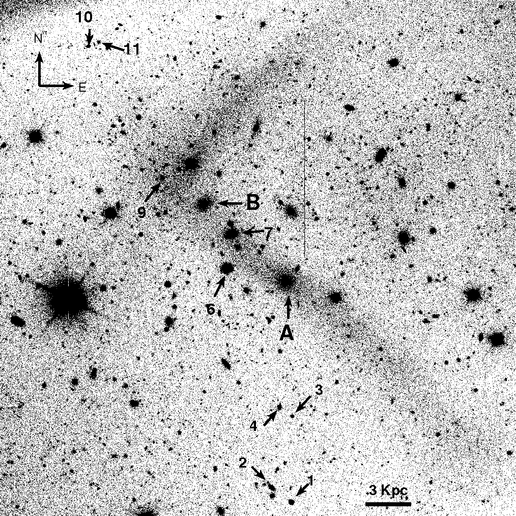
Figure 1:
FORS2/UT2 400 s Bessel V-band image of NGC 1097's northeast optical jet and ``dog-leg''.
The targets observed spectoscopically with FORS2 are labeled as in Table 1. The figure covers
|
| Open with DEXTER | |
1.1 The nature of NGC 1097's optical ``jet-like'' tidal streams
NGC 1097's network of faint optical ``jets'' have puzzled astronomers
since their discovery in the mid-1970s (Wolstencroft & Zealey 1975;
Arp 1976; Lorre 1978). These early observations established their
blue optical colors and lack of optical emission lines. The fact that
all four appear to radiate from NGC 1097's Seyfert 1 nucleus (see
Fig. 1 in Lorre 1978 and Fig. 1) led quite naturally to
explanations involving AGN phenomena. However, the sensitive
upper flux limits at 1.4 GHz set by Wolstencroft et al. (1984) with the
Very Large Array (VLA) showed that the ``jets'' optical emission did
not arise through the synchrotron process. Their observations could
not exclude the possibility that the ``jets'' were dominated by
thermal Bremsstrahlung emission from a ![]() 106 K plasma (the
high temperature is required to explain the absence of H
106 K plasma (the
high temperature is required to explain the absence of H![]() emission set by Arp 1976). The same year, Carter et al. (1984, hereafter CAM) proposed a very different interpretation based
on optical and near-infrared surface photometry of the two northern
jets and the most prominent of several optical knots in the northeast
jet first noted by Arp (1976) and Lorre (1978). The colors of the diffuse
light in the northern jets (e.g.,
emission set by Arp 1976). The same year, Carter et al. (1984, hereafter CAM) proposed a very different interpretation based
on optical and near-infrared surface photometry of the two northern
jets and the most prominent of several optical knots in the northeast
jet first noted by Arp (1976) and Lorre (1978). The colors of the diffuse
light in the northern jets (e.g.,
![]() and
and
![]() )
are inconsistent with both thermal Bremsstrahlung and
synchrotron emission. Instead, CAM proposed that the ``jet-like''
features are in fact composed of stars, similar to ordinary disk
populations (
)
are inconsistent with both thermal Bremsstrahlung and
synchrotron emission. Instead, CAM proposed that the ``jet-like''
features are in fact composed of stars, similar to ordinary disk
populations (![]() G-type). These stars either: formed in
situ from the cooling plasma of an ancient radio jet, were drawn out
of NGC 1097's disk through a tidal interaction with its companion
NGC 1097A, or represented the remains of a dwarf irregular or small
spiral galaxy cannibalized by the much larger NGC 1097 (i.e., a minor
merger). CAM went so far as to propose that the prominent optical knot
near the northeast jet's abrupt right-angle bend (called the
``dog-leg'') might be what is left of the dwarf's tidally-stripped
nucleus, given that its color (
G-type). These stars either: formed in
situ from the cooling plasma of an ancient radio jet, were drawn out
of NGC 1097's disk through a tidal interaction with its companion
NGC 1097A, or represented the remains of a dwarf irregular or small
spiral galaxy cannibalized by the much larger NGC 1097 (i.e., a minor
merger). CAM went so far as to propose that the prominent optical knot
near the northeast jet's abrupt right-angle bend (called the
``dog-leg'') might be what is left of the dwarf's tidally-stripped
nucleus, given that its color (
![]() )
is similar to
that of late-type spiral nuclei. Wehrle et al. (1997) used VLA
observations at 327 MHz to conclusively rule out the ``jet-like''
features being a network of ancient radio jets, and they concluded
that NGC 1097's jets are nothing more than a set of unusual tidal
streams created through multiple encounters with the small elliptical
companion NGC 1097A. Since tidal streams, and especially blue
tidal streams, are typically rich in neutral atomic hydrogen gas (HI),
this opened the interesting possibility of using HI kinematics to
explore their origin and evolution.
)
is similar to
that of late-type spiral nuclei. Wehrle et al. (1997) used VLA
observations at 327 MHz to conclusively rule out the ``jet-like''
features being a network of ancient radio jets, and they concluded
that NGC 1097's jets are nothing more than a set of unusual tidal
streams created through multiple encounters with the small elliptical
companion NGC 1097A. Since tidal streams, and especially blue
tidal streams, are typically rich in neutral atomic hydrogen gas (HI),
this opened the interesting possibility of using HI kinematics to
explore their origin and evolution.
Higdon & Wallin (2003, hereafter HW) revived the ``minor merger'' interpretation
for the tidal streams. Using the VLA in its most compact
configuration, they found that all four tidal streams are extremely
gas poor (
![]()
![]() pc-2, 3
pc-2, 3![]() ). Given their blue color, they are unlike any tidal stream in
the literature (cf. Hibbard et al. 2000; Higdon et al. 2006).
The total lack of HI had additional implications: the stars could not
have originated from the
HI rich disk of NGC 1097, nor could they have been formed in
situ from a cooling radio jet without unrealistic star formation
efficiencies. HW proposed a scenario in which the
tidal streams were formed by multiple passes of a gas rich dwarf
galaxy through the center of the much more massive NGC 1097. Their n-body
simulations of such a capture produced features that strikingly
resembled the four optical tidal streams, including the abrupt 90
). Given their blue color, they are unlike any tidal stream in
the literature (cf. Hibbard et al. 2000; Higdon et al. 2006).
The total lack of HI had additional implications: the stars could not
have originated from the
HI rich disk of NGC 1097, nor could they have been formed in
situ from a cooling radio jet without unrealistic star formation
efficiencies. HW proposed a scenario in which the
tidal streams were formed by multiple passes of a gas rich dwarf
galaxy through the center of the much more massive NGC 1097. Their n-body
simulations of such a capture produced features that strikingly
resembled the four optical tidal streams, including the abrupt 90![]() bend of the dog-leg region (see their Figs. 12-14). The
dwarf galaxy's ISM is swept out by ram pressure stripping during its
initial pass through NGC 1097's disk, resulting in the creation of
essentially gas free ``jet-like'' stellar streams. Within the HW picture,
NGC 1097's optical tidal streams represents the late stages
in the cannibalization of a small disk galaxy by a much larger spiral.
bend of the dog-leg region (see their Figs. 12-14). The
dwarf galaxy's ISM is swept out by ram pressure stripping during its
initial pass through NGC 1097's disk, resulting in the creation of
essentially gas free ``jet-like'' stellar streams. Within the HW picture,
NGC 1097's optical tidal streams represents the late stages
in the cannibalization of a small disk galaxy by a much larger spiral.
1.2 Structures in NGC 1097's northeast tidal stream
Arp (1976) and Lorre (1978) noted the presence of several optical
knots near the northeast tidal feature's dog-leg region (see
Figs. 1 and 3) that appeared too blue for
background ellipticals, though with no redshifts available the possibility that
they were background objects could not be ruled out. Wehrle et al. (1997) obtained 4000-7000 Å spectra of the two brightest knots
using 1-2 h exposures with the CTIO 4 m Blanco telescope, and
detected only weak continuum (after averaging over large wavelength
bins) and no measurable line emission (e.g.,
![]() Å and
Å and
![]() ,
,
![]() Å). Because of
detector instabilities, the quality of their spectra was not sufficient
to determine the nature of knots A & B. While it had yet to be
established that the knots were in fact part of the northeast tidal
stream, it was clear from their apparent lack of strong emission lines
that neither were star forming dwarf galaxies or distant AGN. The
existence of multiple knots are of particular interest, as they
might represent ongoing structure formation in the tidal streams.
Å). Because of
detector instabilities, the quality of their spectra was not sufficient
to determine the nature of knots A & B. While it had yet to be
established that the knots were in fact part of the northeast tidal
stream, it was clear from their apparent lack of strong emission lines
that neither were star forming dwarf galaxies or distant AGN. The
existence of multiple knots are of particular interest, as they
might represent ongoing structure formation in the tidal streams.
|
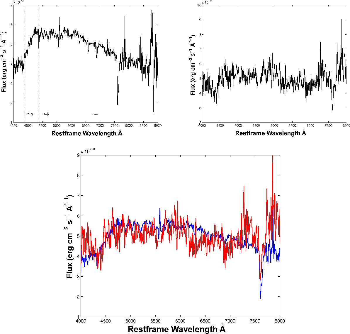
Figure 2: Up left: FORS2 spectrum of knot A. Up right: FORS2 spectrum of knot B. Bottom: comparison of knot A's spectrum (blue line) vs. knot B's (red line). |
| Open with DEXTER | |
In this paper we analyze VLT/FORS2 spectra of
five of the brightest optical knots in the northeast tidal stream. We
show that the most prominent condensation, knot A, has the same
redshift as the spiral NGC 1097, and argue that it is physically
associated with the tidal stream. A second condensation, knot B, is
also plausibly associated with the tidal feature![]() .
.
The VLT observations are described in Sect. 2. In
Sect. 3 we
present the photometric and spectroscopic measurements of knots A
& B, and discuss these findings and their implications in
Sect. 4. Finally, we summarize our results in Sect. 5.
Throughout this
paper we have adopted the standard WMAP cosmology (
![]() km s-1 Mpc-1; Spergel et al. 2003), which for NGC 1097's redshift (
km s-1 Mpc-1; Spergel et al. 2003), which for NGC 1097's redshift (
![]() ,
e.g., Koribalski et al. 2004; Mathewson & Ford 1996) results
in a luminosity distance
,
e.g., Koribalski et al. 2004; Mathewson & Ford 1996) results
in a luminosity distance ![]() of
of ![]() Mpc and a linear scale of
84 pc/
Mpc and a linear scale of
84 pc/
![]() .
.
2 VLT observations and data reduction
The observations were made at ESO-Paranal by
G. Rupprecht and H. Arp (observing program 66.B-0481) on several runs: 7 October 2000 (ID 101443),
17 November 2000 (ID 103791), and 4 December 2000 (ID 103790).
The data were kindly provided by Arp and Rupprecht.
Optical spectra were obtained with the FORS2 imaging-spectrograph
(1998), situated at the Cassegrain focus of the 8.2 m VLT Kueyen
(UT2). The detector was a 2048 ![]() 2048 TK2048EB4-1 thinned, backside illuminated CCD.
The standard resolution collimator was used, providing an angular
scale of 0.2
2048 TK2048EB4-1 thinned, backside illuminated CCD.
The standard resolution collimator was used, providing an angular
scale of 0.2
![]() /pix and a field of view of 6
/pix and a field of view of 6
![]() 8
8 ![]() 6
6
![]() 8.
Grism GRIS_150I+27 was used, which provides a linear dispersion of 230 Å/mm
and
8.
Grism GRIS_150I+27 was used, which provides a linear dispersion of 230 Å/mm
and
![]() (if coupled with a 1
(if coupled with a 1
![]() slit).
Spectra covering the full 3300-1000 Å wavelength range
were obtained in two stages: red spectra (6000-10 000 Å) using the
OG590+32 filter as an order blocker, and blue spectra
(3300-6600 Å)
with no filter.
slit).
Spectra covering the full 3300-1000 Å wavelength range
were obtained in two stages: red spectra (6000-10 000 Å) using the
OG590+32 filter as an order blocker, and blue spectra
(3300-6600 Å)
with no filter.
The observations were carried out in multi-object (MXU) mode, with
twelve slits of varying widths (1
![]() to 2.5
to 2.5
![]() )
placed on the
sky. One large slit was situated across the northeast tidal stream, one slit
each was placed on knots A & B, six on field objects, and three on
empty fields to measure sky emission. The integration time for the spectra was 30 min.
Data reduction was routine,
and standard procedures in IRAF
)
placed on the
sky. One large slit was situated across the northeast tidal stream, one slit
each was placed on knots A & B, six on field objects, and three on
empty fields to measure sky emission. The integration time for the spectra was 30 min.
Data reduction was routine,
and standard procedures in IRAF![]() were used to extract (apall),
calibrate (identify, calibrate), and join (scombine)
the red and blue spectrum for each slit.
See Table 1 for the coordinates,
photometry and a short description of the observed objects.
were used to extract (apall),
calibrate (identify, calibrate), and join (scombine)
the red and blue spectrum for each slit.
See Table 1 for the coordinates,
photometry and a short description of the observed objects.
The spectrum of the northeast tidal stream was too faint to be
successfully extracted with apall. Despite using the largest
available slit and the lowest dispersion grism available, the tidal stream proved too faint
for useful spectroscopy in 30 min of integration. We
obtained, however, well exposed spectra for nine other objects, including
knot A, and a less exposed but still useful spectrum of knot B (see Fig. 2).
FORS2 was also used to obtain a 400 s Bessel V-band exposure
centered on the northeast dog-leg tidal stream (see Fig. 1). The
night's seeing (FWHM of unsaturated stars measured on the image)
was ![]()
![]() .
.
3 Results
3.1 Spectroscopy of the condensations in the ``dog-leg'' tidal stream
The five optical condensations in the northeast tidal stream that were observed
spectroscopically with FORS2 are indicated in Fig. 1 and listed in
Table 1. Of these, one is a foreground star (Object 9) and two are background galaxies
(Objects 6 and 7), with
![]() .
We will not discuss these sources further.
.
We will not discuss these sources further.
A high quality spectrum was extracted for knot A, and is shown in
Fig. 2. The spectrum is notable for a total lack of emission lines
ordinarily found in star forming systems like [O III]
![]() 4959, 5007 Å, H
4959, 5007 Å, H![]() or H
or H![]() ,
in agreement with Arp (1976) and
Wehrle et al. (1997). However, these new observations set more
stringent limits on H
,
in agreement with Arp (1976) and
Wehrle et al. (1997). However, these new observations set more
stringent limits on H![]() emission, with
emission, with
![]() Å . Several narrow hydrogen Balmer absorption lines (H
Å . Several narrow hydrogen Balmer absorption lines (H![]() ,
H
,
H![]() ,
and H
,
and H![]() )
are clearly detected, with equivalent widths
(measured with IRAF's splot tool) of 2.9, 3.8 and 2.3 Å
respectively (see Table 2).
There is also evidence for a weak G-band (
)
are clearly detected, with equivalent widths
(measured with IRAF's splot tool) of 2.9, 3.8 and 2.3 Å
respectively (see Table 2).
There is also evidence for a weak G-band (![]() 4303 Å)
absorption. The most prominent feature in Fig. 2 is a strong break in the
continuum level at
4303 Å)
absorption. The most prominent feature in Fig. 2 is a strong break in the
continuum level at ![]() 4400 Å.
4400 Å.
We derive synthetic optical colors for knot A using the spectrum in Fig. 2
by numerically integrating over the Johnson-Cousins UBVRI passbands, and find
![]() ,
,
![]() ,
,
![]() and
and
![]() .
Note that these colors are somewhat redder than the colors of the local diffuse jet
emission as measured by CAM (
.
Note that these colors are somewhat redder than the colors of the local diffuse jet
emission as measured by CAM (
![]() ). The 1.8
). The 1.8![]() deviation
between our and CAM's measures is not surprising considering the inherent difficulty
in measuring the colors of such a low brightness feature, and the fact that CAM
performed those measures more than 20 yr ago, using normal photographic plates.
deviation
between our and CAM's measures is not surprising considering the inherent difficulty
in measuring the colors of such a low brightness feature, and the fact that CAM
performed those measures more than 20 yr ago, using normal photographic plates.
From the measured wavelengths of absorption lines in knot A's spectrum
(see Table 2) we derive a redshift of
![]() .
This is within
.
This is within
![]() of NGC 1097's redshift
derived using HI and optical emission lines, and shows that knot A is
indeed physically associated with the barred spiral galaxy.
of NGC 1097's redshift
derived using HI and optical emission lines, and shows that knot A is
indeed physically associated with the barred spiral galaxy.
As shown in Fig. 2 (upper-right panel) the two features in the spectrum of knot B,
being possibly significant above the noise are the break in the continuum level
at 4400 Å and the H![]() line at 4882 Å. As is shown in Fig. 2
(bottom panel) the overall continuum shape and the position of these two
features match fairly well those of knot A, indicating that their redshifts could be similar.
Under the assumption that knot B is at the same redshift distance of knot A,
we find moreover that knot B
agree very well with the same photometric scaling relations of knot A. This makes it unlikely
that knot B is a galaxy with a different absolute magnitude than knot A, placed at a different
distance from NGC 1097. We will therefore assume throughout the rest of the article that knot B is
physically associated with NGC 1097.
line at 4882 Å. As is shown in Fig. 2
(bottom panel) the overall continuum shape and the position of these two
features match fairly well those of knot A, indicating that their redshifts could be similar.
Under the assumption that knot B is at the same redshift distance of knot A,
we find moreover that knot B
agree very well with the same photometric scaling relations of knot A. This makes it unlikely
that knot B is a galaxy with a different absolute magnitude than knot A, placed at a different
distance from NGC 1097. We will therefore assume throughout the rest of the article that knot B is
physically associated with NGC 1097.
3.2 Surface photometry and morphology of knots A & B
Both knots A & B in the NE tidal stream are easily seen in the FORS2 V-band
image shown in Fig. 1. We are able to extract new details
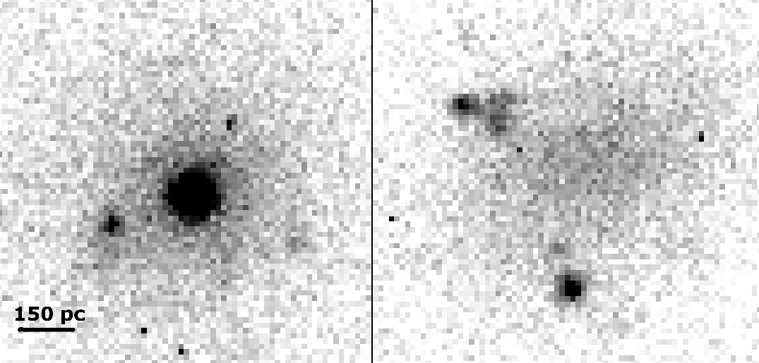
concerning their morphologies: Knot A shows considerable spherical
symmetry, with a bright and compact core and a halo that extends for
the full width of the stream (![]()
![]() ), while knot B is more
diffuse and lacks a central core (see Fig. 3).
), while knot B is more
diffuse and lacks a central core (see Fig. 3).
|
Figure 3:
Closeups (
|
| Open with DEXTER | |
Table 1: Magnitudes of the observed objects: The labels fs, bg, c indicate respectively: ``foreground star'', ``backgroung galaxy'', ``condensation''. The typical rms errors for the magnitudes are 0.1 mag.
Table 2:
Absorption redshift of knot A:
![]() is the measured wavelength,
is the measured wavelength,
![]() is the rest-frame wavelength, z is the measured redshift and
is the rest-frame wavelength, z is the measured redshift and ![]() is
the redshift difference with NGC 1097 (z= 0.0042 NED).
is
the redshift difference with NGC 1097 (z= 0.0042 NED).
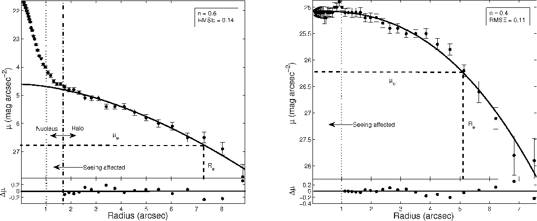
![\begin{displaymath}\mu (R) = \mu_{\rm e} \exp \left\{-b_{n}\left[\left(R \over R_{\rm e}\right)^{1/n}-1\right]\right\},
\end{displaymath}](/articles/aa/full_html/2010/13/aa13518-09/img51.png)
|
(1) |
where R is the projected radial distance from the center of the galaxy. This representation is widely used and has the advantage of precisely describing a variety of SBPs, including pure exponential and de Vaucouleurs R1/4 laws, i.e., those of both dwarf and luminous elliptical galaxies (Faber & Lin 1983; de Vaucouleurs 1948, 1959). The free parameters of this model are
|
Figure 4:
Left: Knot A's surface brightness profile obtained with IRAF's
ellipse task. The continuos line represent the Sérsic n=0.6model fit. The dotted line delimits the seeing affected zone, while the
dash-dotted line is placed at
|
| Open with DEXTER | |
Accurate half-light radii have been computed for both objects. For knot B, we estimate
the half-light radius from the Sérsic model fit to be (see above)
![]() pc, where we have included contributions from the pixel
scale and saturation effects in the uncertainty.
Since knot A's core cannot be fit by a Sérsic profile, we estimate
an empirical half-light radius using the ellipse output to calculate the radius
at which the total flux drops by half. In this way we obtain
pc, where we have included contributions from the pixel
scale and saturation effects in the uncertainty.
Since knot A's core cannot be fit by a Sérsic profile, we estimate
an empirical half-light radius using the ellipse output to calculate the radius
at which the total flux drops by half. In this way we obtain
![]() pc.
pc.
Integrated apparent V-band magnitudes were determined to be
![]() mag and
mag and
![]() mag for knots A & B respectively, which correspond to absolute
magnitudes of
mag for knots A & B respectively, which correspond to absolute
magnitudes of
![]() and
and
![]() at the adopted distance
of NGC 1097. Assuming
at the adopted distance
of NGC 1097. Assuming
![]() (Bell & de Jong 2001), these translate into
V-band luminosities of
(Bell & de Jong 2001), these translate into
V-band luminosities of
![]()
![]() for knot A
and
for knot A
and
![]()
![]() for knot B. We also estimate mV, MV,
and LV for knot A's core using a circular aperture of radius
for knot B. We also estimate mV, MV,
and LV for knot A's core using a circular aperture of radius
![]() ,
and find
,
and find
![]() mag,
mag,
![]() and
and
![]()
![]() .
.
Dwarf galaxies subject to ongoing tidal perturbations may show surface brightness ``breaks'' or other irregularities in their outer isophotes (Peñarrubia et al. 2009). We are however unable to detect such irregularities in our surface brightness profiles (see Fig. 4).
This however does not necessarly imply that the knots are not being tidally stripped, since as shown by Peñarrubia et al. (2009) such ``bumps'' in the isophotes are essentially transient features that quickly drift in the outer region of the SBPs, where the S/N may be too low to give any useful information. Their eventual detection is therefore related to the time of the observation, and strongly depends on the orbital parameters of the tidally-disrupting object. Moreover, it is likely that the spatial resolution of our SBPs is simply insufficient to reveal these ``bumps'': our objects have in fact a very small angular extension if compared to Local Group (LG) dwarfs. It is however difficult to estimate the expected amplitude of these irregularities without knowing the orbit of the objects and their internal kinematics.
|
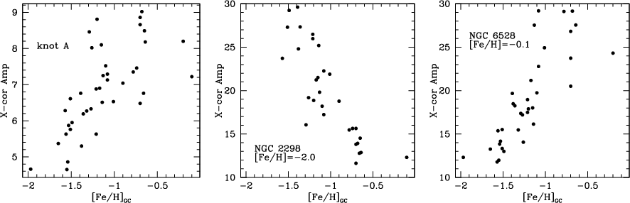
Figure 5: Left: Knot A's cross correlation amplitude as a function of metallicity for galactic GCs from Schiavon (2005). The rough linear relation of positive slope, indicates that our spectrum is better fit by metal-rich than metal-poor GCs (see the text and next figure for details). Center, right: the same as left for two Galactic GCs from the same library, whose metallicity has been estimated with HR spectroscopy. As expected, the metal poor GC NGC 2298 correlates better with metal poor GCs while the metal rich GC NGC 6528 correlates best with metal rich GCs. |
| Open with DEXTER | |

|
Figure 6:
Left: Comparison between knot A's spectrum (continuous line) and the best
correlating GC from Schiavon (2005) (dashed line, cross correlation amplitude 9), which is the intermediate
metallicity GC NGC 6388. Right: the same as left with the worst correlating GC from
Schiavon et al. (2005) (cross correlation amplitude 4.5), which is NGC 1904. The two plots show that knot A's
spectrum correlates best with intermediate to high metallicity GCs like NGC 6388
(
|
| Open with DEXTER | |

|
Figure 7: Absolute magnitudes vs half light radii for local group dwarfs from (Mateo 1998), Galactic globular clusters (Webbink 1985) and the two knots. |
| Open with DEXTER | |
Table 3: Summary of measured and estimated (E) parameters for knots A & B.
3.3 Stellar population
The resolution of knot A's spectrum (
![]() Å at
5000 Å) is too low to accurately estimate metal abundances from
spectral line indices. An estimate of its metallicity would be nonetheless
useful to help constrain its nature.
Å at
5000 Å) is too low to accurately estimate metal abundances from
spectral line indices. An estimate of its metallicity would be nonetheless
useful to help constrain its nature.
In order to extract more information regarding knot A's stellar population, we cross-correlated its spectrum with that of 40 galactic GCs from the library in Schiavon et al. (2005), which covers a wide range of metallicities from -2 dex to solar abundance. We degraded the spectral resolution of the 40 galactic GCs to match that of knot A's spectrum, and used the IRAF task fxcor for cross-correlation.
With this method we find a linear relation between the cross correlation amplitudes of knot A (plus two test GCs) and the [Fe/H] ratios of the library's GCs (see Fig. 5). This is reasonable considering that for evolved stellar populations, the [Fe/H] ratio should play an important role in determining spectral differences. This implies that the [Fe/H] ratio of knot A can be estimated - at least qualitatively - using this cross correlation technique.
The results of the left panel of Fig. 5 imply an [Fe/H] ratio >-1.0 dex for knot A. The analogous plots in the middle and right panel for a metal-poor and a metal-rich GC confirm the validity of this approach, since the slope of the cross-correlation amplitude vs. [Fe/H] is, as expected, negative for the metal-poor and positive for the metal-rich GCs.
Figure 6 confirms the results of Fig. 5 by comparing knot A's spectrum with the two GCs with highest and lowest cross-correlation amplitudes. The match is very good for the GC NGC 6388, which is of intermediate metallicity ([Fe/H] = -0.7 dex), and shows a clear discrepancy for NGC 1904, which has a lower metallicity ([Fe/H] = -1.5 dex). Since NGC 6388 has an integrated spectral type of G2, while NGC 1904 has type F4/5 (Harris et al. 1996), we can state that the light emitted by knot A's is most likely dominated by G-type stars, in agreement with CAM.
While it is true that this method does not precisely determine the [Fe/H] ratio, the results shown in Figs. 5 and 6 indicate (at least qualitatively) that knot A's metal abundances are higher than LG dwarf spheroidals of similar luminosity (e.g., [Fe/H] = -1.5 dex; Mateo 1998). It has been shown however, that dSph galaxies belonging to different clusters of galaxies may show sensible differences in their metallicity-luminosity relation, if compared with LG dwarves (Lianou et al. 2010).
4 Discussion
4.1 Are the knots dwarf spheroidal galaxies?
We have shown that knot A's optical spectrum and total luminosity
matches well that of intermediate to metal rich and massive GCs like 47 Tucanae and
Mayall I. However, the size of knot A (
![]() pc) is abundantly
beyond those of ordinary GCs, the vast majority of which possess
pc) is abundantly
beyond those of ordinary GCs, the vast majority of which possess
![]() pc (cf. Mackey & van den Bergh 2005). In terms of
size both knots A & B are similar to LG dSph satellite galaxies of comparable
luminosity (Mateo 1998). It has been established that dSph galaxies and GCs occupy different
positions in a plot of half-light radius versus
pc (cf. Mackey & van den Bergh 2005). In terms of
size both knots A & B are similar to LG dSph satellite galaxies of comparable
luminosity (Mateo 1998). It has been established that dSph galaxies and GCs occupy different
positions in a plot of half-light radius versus ![]() .
Large GCs
in fact obey a well defined relation, in the sense that larger GCs are
also fainter (
.
Large GCs
in fact obey a well defined relation, in the sense that larger GCs are
also fainter (
![]() ;
Mackey & van den Bergh 2005; though Van den Bergh 2008 discusses shortcomings
of this diagnostic). Knots A & B are well above this line trend (they
are much larger for their optical luminosity than GCs) (see Fig. 7).
Instead, the knots agree very well with the
;
Mackey & van den Bergh 2005; though Van den Bergh 2008 discusses shortcomings
of this diagnostic). Knots A & B are well above this line trend (they
are much larger for their optical luminosity than GCs) (see Fig. 7).
Instead, the knots agree very well with the
![]() relation for LG
and Hydra/Centaurus dwarves (Misgeld et al. 2008, 2009).
They found that typical dSph galaxies follow the relation (cf. Misgeld et al. 2009):
relation for LG
and Hydra/Centaurus dwarves (Misgeld et al. 2008, 2009).
They found that typical dSph galaxies follow the relation (cf. Misgeld et al. 2009):
| (2) |
Substituting
In terms of stellar population (old GC-like stellar population with no signs of ongoing SF and a
peculiar lack of HI), stellar mass (
![]() for knot A and
for knot A and
![]() for knot B), central surface brightness and Sérsic
index (see above), Mv vs R50 (see Fig. 7) our knots closely resemble ordinary dSph
galaxies, as defined in Grebel et al. (2003) and Mateo (1998).
for knot B), central surface brightness and Sérsic
index (see above), Mv vs R50 (see Fig. 7) our knots closely resemble ordinary dSph
galaxies, as defined in Grebel et al. (2003) and Mateo (1998).
|
Figure 8:
Left: in this ehnanced version of Fig. 1 (3
|
| Open with DEXTER | |
4.2 Structure and composition of the stellar stream
The stellar stream itself was too faint for quantitative spectroscopy.
From our sky-substracted V-band exposure however (see Fig. 1), we could
measure the mean surface brightness of the stream (measured over ten different apertures a
long the ``dog-leg''). The value that we obtained is
![]() mag/arcsec2.
After measuring the mean SB of the stream using the standard IRAF tools, authors PG and SM
independently measured the size of the stream, by subdividing it in small rectangular apertures.
The value found is
mag/arcsec2.
After measuring the mean SB of the stream using the standard IRAF tools, authors PG and SM
independently measured the size of the stream, by subdividing it in small rectangular apertures.
The value found is
![]() arcsec2. From the measurement of the stream's mean surface
brightness and its area, we have calculated its integrated V magnitude to be
arcsec2. From the measurement of the stream's mean surface
brightness and its area, we have calculated its integrated V magnitude to be
![]() mag. At the distance of NGC 1097 this corresponds to an absolute
magnitude of
mag. At the distance of NGC 1097 this corresponds to an absolute
magnitude of
![]() mag.
mag.
Useful hints about the composition of the tidal stream can be found in earlier studies
(CAM, HW, Wehrle et al. 1997). Using multiband photometry of the tidal stream (obtained in a region
slightly south-western than knot A) CAM suggested that the SED of the ``dog-leg''
feature is compatible with G-type stars.
They also found that the colors of the stream and knot A are similar within
the photometric uncertainties (
![]() ,
,
![]() ).
This last point agrees with the conclusions of Wehrle et al. (1997).
In their paper they measured the B/V count ratio longitudinally and transversally
along the tidal stream (see their Fig. 8), and concluded:
``The color (along the tidal stream) is constant within the errors, including both prominent
condensations''.
Both studies came to the conclusion that the stellar stream is composed of stars near G-type,
and that the stream and the knots have the same color. With our FORS2 spectra, we independently
showed that also knot A is predominantly composed of stars near G-type. This suggests that the
knots and the tidal stream are both composed of the same stellar material.
).
This last point agrees with the conclusions of Wehrle et al. (1997).
In their paper they measured the B/V count ratio longitudinally and transversally
along the tidal stream (see their Fig. 8), and concluded:
``The color (along the tidal stream) is constant within the errors, including both prominent
condensations''.
Both studies came to the conclusion that the stellar stream is composed of stars near G-type,
and that the stream and the knots have the same color. With our FORS2 spectra, we independently
showed that also knot A is predominantly composed of stars near G-type. This suggests that the
knots and the tidal stream are both composed of the same stellar material.
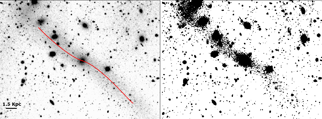
A morphological analysis of the tidal stream indicates that knot A is currently being tidally stripped, populating the ``dog-leg'' tidal stream with stars. As shown in Fig. 8 (left), the tidal stream shows a slight but significant ``S'' shaped inflection coincident with the position of knot A. In Fig. 8 (right), we show moreover the elliptical overdensity of stars at knot A's position. These morphological features are typical for tidally disrupting systems (Forbes et al. 2003; Martínez-Delgado et al. 2008, 2010).
If knot A is the only progenitor of the stellar stream, before the encounter with NGC 1097, knot A
should have been a dwarf galaxy of at least
![]() mag. This means that knot A has lost
at least the 95% of its stars during the encounter with NGC 1097. This is in agreement with the n-body
simulations performed by HW.
mag. This means that knot A has lost
at least the 95% of its stars during the encounter with NGC 1097. This is in agreement with the n-body
simulations performed by HW.
4.3 How did the knots form?
The alignment of knots A & B with the ``dog-leg'' tidal stream suggests that these two objects are probably correlated in phase-space. Such a perfect alignment along the same stream would be in fact very unlikely for independently infalling CDM-Subhalos.
A possible explaination to the phase-space correlation problem of Milky Way satellites (Kroupa et al. 2005; Metz et al. 2009a), has been proposed in terms of a ``group infall'' of sub-halos (Li & Helmi 2008; D'Onghia & Lake 2008; D'Onghia et al. 2009). Alternately, dwarf galaxies may form along dark matter filaments (Ricotti et al. 2008). It is, however, still unclear if these mechanisms can efficiently explain the observed distribution of satellite galaxies around the Milky Way and Andromeda (for recent criticism see: Metz et al. 2009b,a).
The alignment of knots A & B with the stream is instead reminescent of the situation in the Milky Way, where the disk-of-satellites is approximately aligned with the Magellanic Stream (Metz et al. 2009b). This may suggest that the satellite galaxies of NGC 1097 may also be interpreted as being old tidal dwarf galaxies (Zwicky 1956; Lynden-Bell 1983; Okazaki & Taniguchi 2000).
However, a definitive interpretation awaits further study, in particular, we need to examine both knots' internal kinematics, and whether NGC 1097 has additional dSph satellite galaxies. The deep implications for fundamental physics of objects such as knots A & B being tidal dwarf galaxies are discussed in Kroupa et al. (2010).
5 Conclusions
We have shown that the two optical ``knots'' along NGC 1097's tidal stream share most of their observable properties with ordinary dwarf spheroidal galaxies (dSphs). From the measured redshifts we show that knot A (and very likely knot B) are associated with the tidal stream. The spectral light distribution of these dSphs is most consistent with that of intermediate to metal-rich Galactic GCs (see Figs. 6, 7).
These new observations set more stringent limits for H![]() emission of
the tidal stream, with EW
emission of
the tidal stream, with EW
![]() Å.
Å.
Our new observations, togheter with the results from former studies (Carter et al. 1984; Wehrle et al. 1997; Higdon & Wallin 2003), indicate that knot A is composed of the same stellar material as the tidal stream. Moreover, a morphological analysis of the tidal stream reveals clear signs of ongoing tidal stripping (see Fig. 8). Based on this evidence we conclude that very likely the stellar stream is populated by stars drawn out from knot A.
The presence of ongoing tidal stripping is incompatible with knot A being surrounded at present by a massive CDM halo (Peñarrubia et al. 2008, 2009).
AcknowledgementsWe wish to thank Halton C. Arp (MPA Garching) and Gero Rupprecht (ESO Garching), E.M. Burbidge and V. Jukkarinen (CASS San Diego) for their useful comments. We wish to extend a special word of thanks to Martino Romaniello (ESO Garching), Dieter Horns and Andrea Santangelo (IAAT Tuebingen) for their help during the preliminary stages of this paper.
References
- Arp, H. 1976, ApJ, 207L,147A [Google Scholar]
- Appenzeller, I., Fricke, K., Frütig, W., et al. 1998, The Messenger, 94, 1 [NASA ADS] [Google Scholar]
- Bekki, K., Couch, W. J., Drinkwater, M. J., & Shioya, Y. 2003a, MNRAS, 344, 399 [NASA ADS] [CrossRef] [Google Scholar]
- Bekki, K., Forbes, D. A., Beasley, M. A., & Couch, W. J. 2003b, MNRAS, 344, 1334 [Google Scholar]
- Bell, E. F., & de Jong, R. S. 2001, ApJ, 550, 212 [NASA ADS] [CrossRef] [Google Scholar]
- Bruzual, G., & Charlot, S. 2003, MNRAS, 344, 1000B [NASA ADS] [CrossRef] [Google Scholar]
- Carter, D., Allen, D. A., & Malin, D. F. 1984, MNRAS, 211, 707 [NASA ADS] [Google Scholar]
- Capaccioli, M. 1987 in Structure and Dynamics of Elliptical Galaxies, ed. P. T. de Zeeuw (Dordrecht: Reidel), IAU Symp., 127, 47 [Google Scholar]
- Dekel, A., & Silk, J. 1986 ApJ, 303, 39 [Google Scholar]
- D'Onghia, E., & Lake, G. 2008, ApJ, 686, L61 [NASA ADS] [CrossRef] [Google Scholar]
- D'Onghia, E., Besla, G., Cox, T. J., & Hernquist, L. 2009, Nature, 460, 605 [NASA ADS] [CrossRef] [Google Scholar]
- Duc, P. A., & Mirabel, I. F. 1994, A&A, 289, 83 [NASA ADS] [Google Scholar]
- de Vancouleurs, G. 1948, Ann. d'Astrophysique, 11, 247 [Google Scholar]
- de Vaucouleurs, G. 1959, Handb. Phys., 53, 275 [NASA ADS] [Google Scholar]
- Drinkwater, M. J., Jones, J. B., Gregg, M. D., & Phillipps, S. 2000, PASA, 17, 227 [NASA ADS] [CrossRef] [Google Scholar]
- Faber, S. M., & Lin, D. N. C. 1983, ApJ, 266L, 17F [Google Scholar]
- Fellhauer, M., & Kroupa, P. 2002, MNRAS, 330, 642 [NASA ADS] [CrossRef] [Google Scholar]
- Fellhauer, M., & Kroupa, P. 2005, MNRAS, 359, 223 [NASA ADS] [CrossRef] [Google Scholar]
- Forbes, D., Beasley, M. A., Bekki, K., Brodie, J. P., & Strader, J. 2003, Science, 301, 1217F [NASA ADS] [CrossRef] [Google Scholar]
- Genzel, R. et al. 2006, Nature, 442, 17 [Google Scholar]
- Graham, A. W. 2001, AJ, 121, 820 [NASA ADS] [CrossRef] [Google Scholar]
- Graham, A. W., & Guzman, R. 2003, ApJ, 125, 2936 [Google Scholar]
- Gratton, R. G., et al. 2003, A&A, 408, 592 [Google Scholar]
- Grebel, E. K., Gallagher, J. S., III, & Harbeck, D. 2003, AJ, 125, 1926 [NASA ADS] [CrossRef] [Google Scholar]
- Harris, W. E. 1996, AJ, 112, 1487 [NASA ADS] [CrossRef] [Google Scholar]
- Hasegan, M., Jordán, A., Côté, P., et al. 2005, ApJ, 627, 203 [NASA ADS] [CrossRef] [Google Scholar]
- Hibbard, J. E., Guhathakurta, P., van Gorkom, J. H., & Schweizer, F. 1994, AJ, 107, 67 [NASA ADS] [CrossRef] [Google Scholar]
- Higdon, J. L., & Wallin, J. F. 2003, ApJ, 585, 281 (HW) [NASA ADS] [CrossRef] [Google Scholar]
- Higdon, S. J., Higdon, J. L., & Marshall, J. 2006, ApJ, 640, 768 [NASA ADS] [CrossRef] [Google Scholar]
- Hilker, M., Infante, L., & Richtler, T. 1999, A&AS, 138, 55 [NASA ADS] [CrossRef] [EDP Sciences] [Google Scholar]
- Hilker, M., Infante, L., Vieira, G., Kissler-Patig, M., & Richtler, T. 1999, A&AS, 134, 75 [NASA ADS] [CrossRef] [EDP Sciences] [Google Scholar]
- Hilker, M., Kissler-Patig, M., Richtler, T., Infante, L., & Quintana, H. 1999, A&AS, 134, 59 [Google Scholar]
- Kissler-Patig, M., Jordan, A., & Bastian, N. 2006, A&A, 448, 1031 [NASA ADS] [CrossRef] [EDP Sciences] [Google Scholar]
- Koribalski, B., Staveley-Smith, L., Kilborn, V. A., et al. 2004, AJ, 128, 16 [NASA ADS] [CrossRef] [Google Scholar]
- Kormendy, J., Fisher, D. B., Cornell, M. E., & Bender, R. 2009, ApJS, 182, 216 [NASA ADS] [CrossRef] [Google Scholar]
- Kroupa, P. 1997, New Astron., 2, 139, 164 [NASA ADS] [CrossRef] [Google Scholar]
- Kroupa, P., Theis, C., & Boily C. M. 2005, A&A, 2, 431, 517K [Google Scholar]
- Kroupa, P., et al. 2010, A&A, in press [Google Scholar]
- Lasker, B. M., Sturch, C. R., McLean, B. J., et al. 1990, AJ, 99, 2019 [NASA ADS] [CrossRef] [Google Scholar]
- Lorre, J., J. 1978, ApJ, 222, 99 [NASA ADS] [CrossRef] [Google Scholar]
- Li, Y., & Helmi, A. 2008 MNRAS, 385, 1365 [Google Scholar]
- Lianou, S., Grebel, E. K., & Koch, A. 2010 A&A, in press [Google Scholar]
- Lynden-Bell, D., & Lynden-Bell, R. M. 1995, MNRAS, 275, 429 [NASA ADS] [Google Scholar]
- Mackey, A. D., & van den Bergh, S. 2005, MNRAS, 360, 631 [NASA ADS] [CrossRef] [Google Scholar]
- Maraston, C., Bastian, N., Saglia, R. P., et al. 2004, A&A, 416, 467 [NASA ADS] [CrossRef] [EDP Sciences] [Google Scholar]
- Martinez-Delgado, D., Jay Gabany, R., Crawford, K., et al. 2010, ApJL, submitted [arXiv:1003.4860] [Google Scholar]
- Martínez-Delgado, D., Peñarrubia, J., Gabany, R. J., et al. 2008, ApJ, 689, 184M [CrossRef] [Google Scholar]
- Mateo, M. 1998, ARA&A, 435, 506 [Google Scholar]
- Mathewson, D., & Ford, V. 1996, ApJS, 107, 97 [NASA ADS] [CrossRef] [Google Scholar]
- Metz, M., & Kroupa, P. 2007 MNRAS, 376, 387 [Google Scholar]
- Metz, M., Kroupa, P., & Jerjen, H. 2009a, MNRAS, 394, 2223 [NASA ADS] [CrossRef] [Google Scholar]
- Metz, M., Kroupa, P., Theis, C., Hensler, G., & Jerjen, H. 2009b, ApJ, 697, 269 [NASA ADS] [CrossRef] [Google Scholar]
- Meylan, G., Mayor, M., Duquennoy, A., & Dubath, P. 1995, A&A, 303, 761 [NASA ADS] [Google Scholar]
- Meylan, G., Sarajedini, A., Jablonka, P., et al. 2001, ApJ, 122, 830 [Google Scholar]
- Mieske, S., et al. 2006, ApJ, 131, 2242 [Google Scholar]
- Mirabel, I. F., Dottori, H., & Lutz, D. 1992, A&A, 256, L19 [NASA ADS] [Google Scholar]
- Misgeld, I., Hilker, M., & Mieske, S. 2008, A&A, 486, 697 [NASA ADS] [CrossRef] [EDP Sciences] [Google Scholar]
- Misgeld, I., Hilker, M., & Mieske, S. 2009, A&A, 496, 683 [NASA ADS] [CrossRef] [EDP Sciences] [Google Scholar]
- Monet, D. G., Levine, S. E., Canzian, B., et al. 2003, AJ, 125, 984 [NASA ADS] [CrossRef] [Google Scholar]
- Meylan, G., & Mayor, M. 1986, A&A, 166, 122 [NASA ADS] [Google Scholar]
- Okazaki, T., & Taniguchi, Y. 2000 ApJ, 543, 149 [Google Scholar]
- Patat, F. 2003, From twilight to highlight: the physics of Supernovae, ed. W. Hillebrandt, & B. Leibundgut (Springer), 321 [Google Scholar]
- Peñarrubia, J., McConnachie, A. W., & Navarro, J. F. 2008, ApJ, 673, 226 [NASA ADS] [CrossRef] [Google Scholar]
- Peñarrubia, J., Navarro, J. F., McConnachie, A. W., & Martin, N. F. 2009, ApJ, 698, 222 [NASA ADS] [CrossRef] [Google Scholar]
- Phillips, S., Drinkwater, M. J., Gregg, M. D., & Jones, J. B. 2001, ApJ, 560, 201 [NASA ADS] [CrossRef] [Google Scholar]
- Prieto, M., Maciejewski, W., & Reunanen, J. 2005, AJ, 130, 1472 [NASA ADS] [CrossRef] [Google Scholar]
- Ricotti, M., Gnedin, N. Y., & Shull, J. M. 2008, ApJ, 685, 21 [NASA ADS] [CrossRef] [Google Scholar]
- Scarpa, R. 2006, unpublished [arXiv:astro-ph/0504051] [Google Scholar]
- Schweizer, F. 1982, ApJ, 252, 455 [NASA ADS] [CrossRef] [Google Scholar]
- Schiavon, R. P., Rose, J. A., Courteau, S., & MacArthur, L. A. 2005, ApJS, 160, 163 [NASA ADS] [CrossRef] [Google Scholar]
- Sèrsic, J. L. 1968, Atlas de galaxias australes (Cordoba, Argentina: Observatorio Astronomico) [Google Scholar]
- Spergel, N. D., Verde, L., Peiris, H. V., et al. 2003, ApJS, 148, 175 [NASA ADS] [CrossRef] [Google Scholar]
- Storchi-Bergmann, T., Nemmen, R. S., Spinelli, P. F., et al. 2005, ApJ, 624, 13S [Google Scholar]
- Webbink, R. F. 1985, Dynamics of Star Clusters, ed. J. Goedman, & P. Hut, IAU Symp., 113, 541 [Google Scholar]
- Wehrle, A. E., Keel, W. C., & Jones, D. L. 1997, AJ, 114, 115 [NASA ADS] [CrossRef] [Google Scholar]
- Wolstencroft, R. D., Tully, R. B., & Perley, R. A. 1984, MNRAS, 207, 889 [NASA ADS] [Google Scholar]
- Knierman, K. A., Gallagher, S. C., Charlton, J. C., et al. 2003, AJ, 126, 1227 [NASA ADS] [CrossRef] [Google Scholar]
- Vazdekis, A. 1999, ApJ, 513, 224 [NASA ADS] [CrossRef] [Google Scholar]
- Zwicky, F. 1956, Ergenisse Exakten Naturwissenschaften, 29, 344 [Google Scholar]
Footnotes
- ... stream
- Based on observations made with ESO telescopes at Paranal Observatory in the observing program 66.B-0481 (G. Rupprecht/ H. Arp).
- ... feature
- knots A & B referred to in this paper correspond to the two optical knots discussed in Wehrle et al. (1997). Our knot A is also the ``bright condensation'' in jet R1 discussed by CAM (see their Sect. 3 and Table 2).
- ... IRAF
- IRAF is distributed by the National Optical Astronomy Observatories, which are operated by the Association of Universities for Research in Astronomy, under contract with the National Science Foundation.
All Tables
Table 1: Magnitudes of the observed objects: The labels fs, bg, c indicate respectively: ``foreground star'', ``backgroung galaxy'', ``condensation''. The typical rms errors for the magnitudes are 0.1 mag.
Table 2:
Absorption redshift of knot A:
![]() is the measured wavelength,
is the measured wavelength,
![]() is the rest-frame wavelength, z is the measured redshift and
is the rest-frame wavelength, z is the measured redshift and ![]() is
the redshift difference with NGC 1097 (z= 0.0042 NED).
is
the redshift difference with NGC 1097 (z= 0.0042 NED).
Table 3: Summary of measured and estimated (E) parameters for knots A & B.
All Figures
|
|
Figure 1:
FORS2/UT2 400 s Bessel V-band image of NGC 1097's northeast optical jet and ``dog-leg''.
The targets observed spectoscopically with FORS2 are labeled as in Table 1. The figure covers
|
| Open with DEXTER | |
| In the text | |
|
|
Figure 2: Up left: FORS2 spectrum of knot A. Up right: FORS2 spectrum of knot B. Bottom: comparison of knot A's spectrum (blue line) vs. knot B's (red line). |
| Open with DEXTER | |
| In the text | |
|
|
Figure 3:
Closeups (
|
| Open with DEXTER | |
| In the text | |
|
|
Figure 4:
Left: Knot A's surface brightness profile obtained with IRAF's
ellipse task. The continuos line represent the Sérsic n=0.6model fit. The dotted line delimits the seeing affected zone, while the
dash-dotted line is placed at
|
| Open with DEXTER | |
| In the text | |
|
|
Figure 5: Left: Knot A's cross correlation amplitude as a function of metallicity for galactic GCs from Schiavon (2005). The rough linear relation of positive slope, indicates that our spectrum is better fit by metal-rich than metal-poor GCs (see the text and next figure for details). Center, right: the same as left for two Galactic GCs from the same library, whose metallicity has been estimated with HR spectroscopy. As expected, the metal poor GC NGC 2298 correlates better with metal poor GCs while the metal rich GC NGC 6528 correlates best with metal rich GCs. |
| Open with DEXTER | |
| In the text | |
|
|
Figure 6:
Left: Comparison between knot A's spectrum (continuous line) and the best
correlating GC from Schiavon (2005) (dashed line, cross correlation amplitude 9), which is the intermediate
metallicity GC NGC 6388. Right: the same as left with the worst correlating GC from
Schiavon et al. (2005) (cross correlation amplitude 4.5), which is NGC 1904. The two plots show that knot A's
spectrum correlates best with intermediate to high metallicity GCs like NGC 6388
(
|
| Open with DEXTER | |
| In the text | |
|
|
Figure 7: Absolute magnitudes vs half light radii for local group dwarfs from (Mateo 1998), Galactic globular clusters (Webbink 1985) and the two knots. |
| Open with DEXTER | |
| In the text | |
|
|
Figure 8:
Left: in this ehnanced version of Fig. 1 (3
|
| Open with DEXTER | |
| In the text | |
Copyright ESO 2010
Current usage metrics show cumulative count of Article Views (full-text article views including HTML views, PDF and ePub downloads, according to the available data) and Abstracts Views on Vision4Press platform.
Data correspond to usage on the plateform after 2015. The current usage metrics is available 48-96 hours after online publication and is updated daily on week days.
Initial download of the metrics may take a while.