| Issue |
A&A
Volume 521, October 2010
|
|
|---|---|---|
| Article Number | A13 | |
| Number of page(s) | 9 | |
| Section | Galactic structure, stellar clusters, and populations | |
| DOI | https://doi.org/10.1051/0004-6361/200913087 | |
| Published online | 14 October 2010 | |
Comet-shaped sources at the Galactic center
Evidence of a wind from the central 0.2 pc
K. Muzic1,![]() - A. Eckart1,2
- R. Schödel3 - R. Buchholz1
- M. Zamaninasab1,2 - G. Witzel1
- A. Eckart1,2
- R. Schödel3 - R. Buchholz1
- M. Zamaninasab1,2 - G. Witzel1
1 - Physikalisches Institut, Universität zu Köln, Zülpicher Str. 77,
50937 Köln, Germany
2 - Max-Planck-Institut für Radioastronomie, Auf dem Hügel 69, 53121
Bonn, Germany
3 - Instituto de Astrofísica de Andalucía CSIC, Glorieta de la
Astronoma S/N, 18008 Granada, Spain
Received 7 August 2009 / Accepted 31 May 2010
Abstract
Context. In 2007 we reported two comet-shaped
sources in the vicinity of Sgr A* (0.8
![]() and 3.4
and 3.4
![]() projected distance), named X7 and X3. The symmetry axes of the
two sources are aligned to within 5
projected distance), named X7 and X3. The symmetry axes of the
two sources are aligned to within 5![]() in the plane of the sky, and the tips of their bow shocks point towards
Sgr A*. Our measurements show that the proper motion vectors
of both features are pointing in directions more than 45
in the plane of the sky, and the tips of their bow shocks point towards
Sgr A*. Our measurements show that the proper motion vectors
of both features are pointing in directions more than 45![]() away from the line that connects them with Sgr A*. This
misalignment of the bow-shock symmetry axes and their proper motion
vectors, combined with the high proper motion velocities of several
100 km s-1, suggest that the
bow shocks must be produced by an interaction with some external fast
wind, possibly coming from Sgr A*, or from stars in its
vicinity.
away from the line that connects them with Sgr A*. This
misalignment of the bow-shock symmetry axes and their proper motion
vectors, combined with the high proper motion velocities of several
100 km s-1, suggest that the
bow shocks must be produced by an interaction with some external fast
wind, possibly coming from Sgr A*, or from stars in its
vicinity.
Aims. We have developed a bow-shock model to fit the
observed morphology and constrain the source of the external wind.
Methods. The result of our modeling gives the best
solution for bow-shock standoff distances for the two features, which
allows us to estimate the velocity of the external wind, making certain
that all likely stellar types of the bow-shock stars are considered.
Results. We show that neither of the two bow shocks
(one of which is clearly associated with a stellar source) can be
produced by the influence of a stellar wind of a single mass-losing
star in the central parsec. Instead, an outflow carrying a momentum
comparable to the one contributed by the ensemble of the massive young
stars can drive shock velocities capable of producing the observed
comet-shaped features. We argue that a collimated outflow arising
perpendicular to the plane of the clockwise rotating stars (CWS) can
easily account for the two features and the mini-cavity. However, the
collective wind from the CWS has a scale of >10''. The presence
of a strong, mass-loaded outbound wind at projected distances from
Sgr A* of <1'' in fact agrees with models that predict
a highly inefficient accretion onto the central black hole owing to a
strongly radius dependent accretion flow.
Key words: Galaxy: center - stars: mass-loss - infrared: stars - infrared: ISM
1 Introduction
Analyses of stellar orbits in the central arcsecond of the Milky Way have provided indisputable evidence that the central object at the position of the radio source Sagittarius A* (Sgr A*) is a supermassive black hole (SMBH, e.g. Schödel et al. 2003; Ghez et al. 2008,2005; Gillessen et al. 2009; Eckart et al. 2002; Eisenhauer et al. 2005). Sgr A* is located at the distance ofThe streamers of gas and dust in the central few parsecs
of the Galaxy show a bubble-like region of lower density
(called mini-cavity), located ![]() 3.5'' southwest of
Sgr A*. It
was first pointed out on cm-radio
maps by Yusef-Zadeh et al.
(1990). The strong Fe[III] line
emission seen toward that region (Lutz et al. 1993; Eckart
et al. 1992) is consistent with gas excited by a
collision with a fast
(
3.5'' southwest of
Sgr A*. It
was first pointed out on cm-radio
maps by Yusef-Zadeh et al.
(1990). The strong Fe[III] line
emission seen toward that region (Lutz et al. 1993; Eckart
et al. 1992) is consistent with gas excited by a
collision with a fast
(![]() 1000
km s-1) wind from a source within the
central few arcseconds
(Yusef-Zadeh
& Wardle 1993; Yusef-Zadeh & Melia 1992).
1000
km s-1) wind from a source within the
central few arcseconds
(Yusef-Zadeh
& Wardle 1993; Yusef-Zadeh & Melia 1992).
|
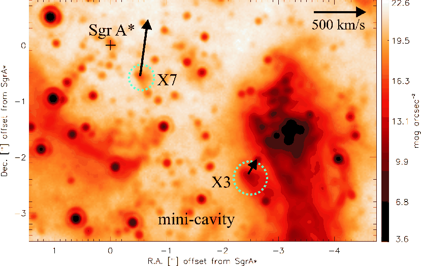
Figure 1:
NACO L'-band (3.8 |
| Open with DEXTER | |
In Muzic et al. (2007)
we presented NACO/VLT multi-epoch observations at 3.8![]() m (L'-band)
which
allowed us to derive proper motions of narrow filamentary features
associated with the gas and dust
streamers of the mini-spiral. Proper motions of several
bow-shock sources have also been reported.
The analysis has shown that the shape and the motion of the filaments
is inconsistent with a
purely Keplerian motion of the gas in the potential
of Sgr A* and that additional mechanisms must be responsible
for their formation
and motion. We argued that the properties of the filaments are probably
related to
an outflow from the disk of young mass-losing
stars around Sgr A*. In part, the outflow may originate in the
immediate vicinity of the black hole itself.
m (L'-band)
which
allowed us to derive proper motions of narrow filamentary features
associated with the gas and dust
streamers of the mini-spiral. Proper motions of several
bow-shock sources have also been reported.
The analysis has shown that the shape and the motion of the filaments
is inconsistent with a
purely Keplerian motion of the gas in the potential
of Sgr A* and that additional mechanisms must be responsible
for their formation
and motion. We argued that the properties of the filaments are probably
related to
an outflow from the disk of young mass-losing
stars around Sgr A*. In part, the outflow may originate in the
immediate vicinity of the black hole itself.
In Muzic et al.
(2007), we reported the existence of the two comet-shaped
features X3 and X7, located at
projected distances of 3.4'' and 0.8'' from Sgr A*,
respectively.
The symmetry axes of the two bow shocks are almost aligned (within 5![]() )
and point
towards Sgr A* (see Fig. 1). At the same
time, their proper motion vectors are not pointing in the
direction of the symmetry axes, as would be expected if the bow-shock
shape were produced
by a supersonic motion of a mass-losing star through a static
interstellar medium. In general,
bow-shock appearance can also be produced by an external supersonic
wind
interacting with a slower wind from
a mass-losing star. If the velocity contrast of the two winds is high,
one will observe
a bow shock pointing towards the source of the external wind.
If in addition the star moves in a different direction than the
position
of the external wind, the bow shock will point in the direction
of the relative velocity between the star and the incident medium.
)
and point
towards Sgr A* (see Fig. 1). At the same
time, their proper motion vectors are not pointing in the
direction of the symmetry axes, as would be expected if the bow-shock
shape were produced
by a supersonic motion of a mass-losing star through a static
interstellar medium. In general,
bow-shock appearance can also be produced by an external supersonic
wind
interacting with a slower wind from
a mass-losing star. If the velocity contrast of the two winds is high,
one will observe
a bow shock pointing towards the source of the external wind.
If in addition the star moves in a different direction than the
position
of the external wind, the bow shock will point in the direction
of the relative velocity between the star and the incident medium.
In this paper we present new proper motion measurements for the two comet-shaped sources X3 and X7 (Sect. 3). In Sect. 4 we explain details of the bow-shock modeling that was used to fit those features (Sect. 5). Possible thee-dimensional positions of the sources are discussed in Sect. 6. In Sect. 7 we argue about the nature of the two sources and the external wind held responsible for the observed arrangement. Summary and conclusions are given in Sect. 8.
2 Observations and data reduction
The L' (3.8 ![]() m)
images were taken with the NAOS/CONICA adaptive optics-assisted
imager/spectrometer
(Rousset
et al. 1998; Lenzen et al. 1998; Brandner
et al. 2002)
at the UT4 (Yepun) at the ESO VLT.
The data set includes images from 7 epochs
(2002.66, 2003.36, 2004.32, 2005.36, 2006.41, 2007.25 and 2008.40)
with a resolution of
m)
images were taken with the NAOS/CONICA adaptive optics-assisted
imager/spectrometer
(Rousset
et al. 1998; Lenzen et al. 1998; Brandner
et al. 2002)
at the UT4 (Yepun) at the ESO VLT.
The data set includes images from 7 epochs
(2002.66, 2003.36, 2004.32, 2005.36, 2006.41, 2007.25 and 2008.40)
with a resolution of ![]() 100 mas
and a pixel scale of 27 mas/pixel.
Data reduction (bad pixel correction, sky subtraction, flat field
correction)
and formation of final mosaics was performed using the DPUSER software
for
astronomical image analysis (T. Ott; see also Eckart
& Duhoux 1990).
100 mas
and a pixel scale of 27 mas/pixel.
Data reduction (bad pixel correction, sky subtraction, flat field
correction)
and formation of final mosaics was performed using the DPUSER software
for
astronomical image analysis (T. Ott; see also Eckart
& Duhoux 1990).
3 Proper motions
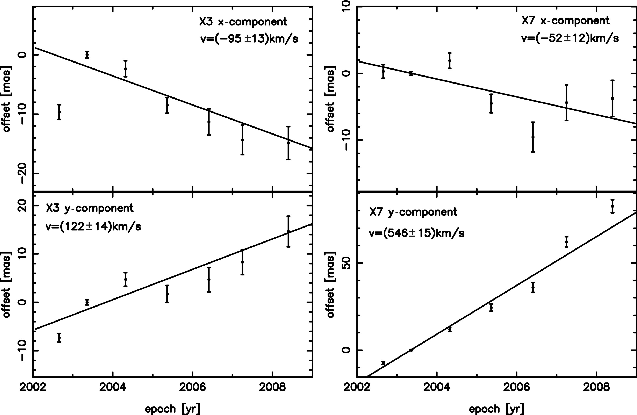
|
Figure 2:
L'-band proper motions of the two comet-shaped
features X3 and X7. The error bars show the 1 |
| Open with DEXTER | |
To obtain proper motions of extended features we used the
same method as described in detail in Muzic
et al. (2007).
Our measurements are shown in Fig. 2. The distance to
the GC was assumed to be 8 kpc.
The results obtained from the L'-band data between
2002 and 2008, are as follows.
X7:
![]() km s-1,
km s-1,
![]() km s-1.
X3:
km s-1.
X3:
![]() km s-1,
km s-1,
![]() km s-1.
The uncertainties are 1
km s-1.
The uncertainties are 1![]() uncertainties of the weighted linear fit to the
positions vs. time.
The proper motion velocity vectors of both sources are
oriented in the northwest quadrant (see Fig. 1).
The results agree with results given in Table 1 of
Muzic et al. (2007),
but
there is an error in their Fig. 5, where X3 is plotted as
moving towards the northeast.
uncertainties of the weighted linear fit to the
positions vs. time.
The proper motion velocity vectors of both sources are
oriented in the northwest quadrant (see Fig. 1).
The results agree with results given in Table 1 of
Muzic et al. (2007),
but
there is an error in their Fig. 5, where X3 is plotted as
moving towards the northeast.
The L-band feature X7 is coincident (in
projection) with a K-band source S 50 (Gillessen et al. 2009).
The reported proper motion of S 50 is ![]() ) km s-1
and
) km s-1
and
![]() km s-1.
While the orientations of the two proper motions agree, there is a
significant difference in proper motion magnitudes.
This, however, might give us an idea
about the systematic uncertainties of the proper motions derived from
the L-band extended sources.
It seems reasonable to argue that we are not dealing with an accidental
superposition of a stellar source with a dust blob along the line of
sight, but that the L-band feature
is indeed associated with the stellar source at the same position.
km s-1.
While the orientations of the two proper motions agree, there is a
significant difference in proper motion magnitudes.
This, however, might give us an idea
about the systematic uncertainties of the proper motions derived from
the L-band extended sources.
It seems reasonable to argue that we are not dealing with an accidental
superposition of a stellar source with a dust blob along the line of
sight, but that the L-band feature
is indeed associated with the stellar source at the same position.
4 Model
4.1 Analytic solution for the bow-shock shape
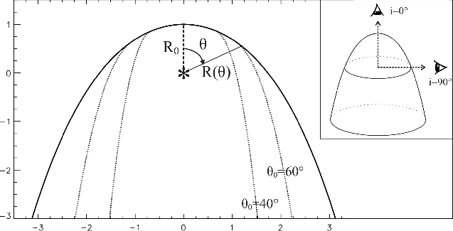
|
Figure 3:
The 2D bow-shock shape.
Full line shows the analytic model from Wilkin
(1996, see Eq. (1). Dotted
lines show narrow solutions (Zhang
& Zheng 1997), for two collimation angles |
| Open with DEXTER | |
Wilkin (1996) derived a
fully analytic solution for the shape of
a bow shock produced by a star moving through the interstellar medium
at supersonic velocity (see Fig. 3).
The 2D shell shape is given by
where
Here,
We assume that the shell has a thickness as shown in Fig. 3b in Mac Low et al. (1991). Then we rotate the 2D shape around its axis of symmetry to obtain the 3D shell.
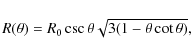
4.2 Narrow solution for the bow-shock shape
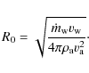
The model by Wilkin (1996) incorporates the instantaneous cooling approximation: the interaction between the stellar wind and the ambient medium takes place in an infinitely thin layer, where the two flows are fully mixed and immediately cooled. In this case R0 directly gives the distance of the star to the apex of the bow shock. However, Comerón & Kaper (1998) point out that this might not be true if cooling of the shocked stellar wind is inefficient. In this case it is expected that the bow shock would be located at a distance somewhat greater than R0(Povich et al. 2008; Comerón & Kaper 1998; Raga et al. 1997). For some GC sources, Tanner et al. (2005) indeed report that a better fit can be obtained if the apex of the bow shock is shifted away from the star. We have observed the same behavior for several other GC bow shocks.
Zhang & Zheng
(1997) have investigated the case where the wind ejection
from the star is not
necessarily isotropic. It is instead confined in a cone of solid angle ![]() ,
where
2
,
where
2![]() is the opening angle in which the matter is ejected. The standoff
distance is then given by
is the opening angle in which the matter is ejected. The standoff
distance is then given by

As can be seen in Fig. 3, with
|
Figure 4:
Results of our modeling for the feature X7 (black contours), observed
in the epoch 2003.36. The image is previously deconvolved and
beam-restored to the nominal resolution of our L'-band
images. Color contours represent the bow-shock model projected onto
the plane of the sky.
|
| Open with DEXTER | |
4.3 Generating emission maps
To generate a simulated observation, we start by illuminating the shell by the star placed at the origin of the coordinate system and then calculate the emission along each ray intersecting the shell. The shell is inclined to the line of sight by the angle i, and also rotated by a position angle PA in the plane parallel to the plane of the sky. The inset in Fig. 3 explains the convention used for the inclination angle. PA is measured east of north.
Each parcel of the shell is assigned the optical depth ![]() ,
calculated as
,
calculated as
|
(4) |
We assume a graphite + silicate mixture with a power-law grain size distribution
The source X7 is polarized (see Muzic
et al. 2007), suggesting that
scattering of the stellar emission by dust particles in the bow-shock
envelope
is probably important. To account for scattering, we proceed in the
following way.
Emission of each parcel of the shell has
contributions both from scattering and thermal emission: ![]() +
+
![]() .
Here,
.
Here,
![]()
![]()
![]() and
and
![]()
![]()
![]() ,
where
d is the distance from the star, B(Td)
is the black body emission at the dust temperature, integrated over
grain sizes, and over wavelengths in our observing band;
,
where
d is the distance from the star, B(Td)
is the black body emission at the dust temperature, integrated over
grain sizes, and over wavelengths in our observing band; ![]() and
and ![]() are
thermal emission and scattering efficiencies, respectively. Dust
temperature at a distance d (in parsecs) from the
star can be calculated as
are
thermal emission and scattering efficiencies, respectively. Dust
temperature at a distance d (in parsecs) from the
star can be calculated as
![]()
![]() L
*,381/6 d
L
*,381/6 d
![]() K (Van Buren
& McCray 1988; Krügel 2003), where
K (Van Buren
& McCray 1988; Krügel 2003), where ![]() is dust grain size in
is dust grain size in ![]() ,
and L*,38 is stellar
luminosity in 1038 erg s s-1.
The (normalized) scattering function,
,
and L*,38 is stellar
luminosity in 1038 erg s s-1.
The (normalized) scattering function, ![]() ,
controls the amount of forward scattering, and
is given by
,
controls the amount of forward scattering, and
is given by
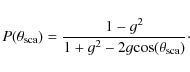
|
(5) |
For g=0, scattering is isotropic, and P does not depend on the scattering angle
Finally, the resulting projection of the 3D-geometry onto the plane of the sky is rebinned to the pixel scale of the NACO images and smoothed with a Gaussian PSF having FWHM equivalent to the angular resolution of our images.
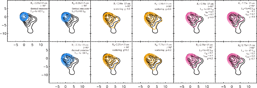
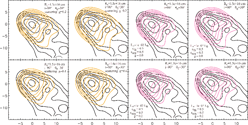
5 Results
5.1 X7
Figure 4
shows the
best-fit results of our bow-shock modeling for the feature X7.
We tested the three different combinations of (
![]() ,
,
![]() ),
and five values of g=(0.0,
0.2, 0.4, 0.6, 0.8). In Fig. 4,
however,
we show only those values that result in good fits, except for the
leftmost
panels, which we show to illustrate the behavior of purely thermal
emission.
Thermal emission is dominant in the vicinity of the star, but cannot
fit the
extended tail that we observe in X7, unless the central star is much
brighter than
the cases investigated here. This, however, is not plausible since X7
is very faint in the K-band (see discussion
below). The tail of the bow shock is described much better by
scattering.
For
),
and five values of g=(0.0,
0.2, 0.4, 0.6, 0.8). In Fig. 4,
however,
we show only those values that result in good fits, except for the
leftmost
panels, which we show to illustrate the behavior of purely thermal
emission.
Thermal emission is dominant in the vicinity of the star, but cannot
fit the
extended tail that we observe in X7, unless the central star is much
brighter than
the cases investigated here. This, however, is not plausible since X7
is very faint in the K-band (see discussion
below). The tail of the bow shock is described much better by
scattering.
For ![]() ,
we only show the solution for L*=102
,
we only show the solution for L*=102 ![]() .
We choose to do so because the difference in resulting contours for the
three stellar luminosities is small, and gives the same solution for
the physically most interesting parameter, R0.
In cases where scattering is important (
.
We choose to do so because the difference in resulting contours for the
three stellar luminosities is small, and gives the same solution for
the physically most interesting parameter, R0.
In cases where scattering is important (
![]() ),
more
forward scattering (large g) results in a more
compact model, thus not fitting well the outer
contours. There is no significant influence of the parameters on the
inner contours, owing to the
relatively small size of the feature and smoothing. These differences
can be better observed in the case of X3.
),
more
forward scattering (large g) results in a more
compact model, thus not fitting well the outer
contours. There is no significant influence of the parameters on the
inner contours, owing to the
relatively small size of the feature and smoothing. These differences
can be better observed in the case of X3.
For each set of parameters (
![]() ,
,
![]() ,
g), we have tested different
values of R0. By changing R0,
the model preserves the same shape of the contours, but is as a whole
expanded or shrunken. Therefore in Fig. 4 we plot two values
of R0 for each set of
parameters. We chose values in the way
that shows how the change in R0
affects the fit. By changing its value by a larger
amount, the fit becomes inadequate.
,
g), we have tested different
values of R0. By changing R0,
the model preserves the same shape of the contours, but is as a whole
expanded or shrunken. Therefore in Fig. 4 we plot two values
of R0 for each set of
parameters. We chose values in the way
that shows how the change in R0
affects the fit. By changing its value by a larger
amount, the fit becomes inadequate.
The best solutions for different sets of parameters are
obtained for ![]() cm,
and
cm,
and ![]() ,
measured east of north.
In this case the best results are
obtained using the simple analytic 2D solution (Eq. (1)).
Both X7 and X3 have an unusually narrow appearance, and therefore are
best
fitted with inclination angles close to 90
,
measured east of north.
In this case the best results are
obtained using the simple analytic 2D solution (Eq. (1)).
Both X7 and X3 have an unusually narrow appearance, and therefore are
best
fitted with inclination angles close to 90![]() .
.
X7 coincides with a point source at shorter wavelengths (see
discussion of
proper motions in Sect. 3).
Photometric measurements give ![]() and
and ![]() (Schödel et al. 2010).
For the local extinction at the position of X7 we assume AK=2.5
(Schödel et al. 2010).
In Sect. 7.1
we discuss possible stellar types and the implications this has on the
external
wind parameters.
(Schödel et al. 2010).
For the local extinction at the position of X7 we assume AK=2.5
(Schödel et al. 2010).
In Sect. 7.1
we discuss possible stellar types and the implications this has on the
external
wind parameters.
5.2 X3
|
Figure 5:
Best-fit results of the modeling for the feature X3 (black contours)
observed in the epoch 2003.36. The image is previously deconvolved and
beam-restored to the nominal resolution of our L'-band
images. Color contours represent the bow-shock model projected onto
the plane of the sky.
|
| Open with DEXTER | |
Figure 5
shows the
best-fit results of our bow-shock modeling for the feature X3.
This feature is very elongated, so a satisfactory fit cannot be
obtained using
the analytic 2D solution. It requires a narrow model (see
Sect. 4.2),
with
small opening angles ![]() .
As in the case of X7, the outer contours are represented better in
models with lower g, while
higher g values result in more compact inner
contours.
Here it is even more evident that thermal emission gives too
compact a model. The elongated tail of X3 can only be well-fitted with
models
that include scattering.
Therefore we only show these solutions, in pairs of two different
values of R0. The best-fit
solutions give
.
As in the case of X7, the outer contours are represented better in
models with lower g, while
higher g values result in more compact inner
contours.
Here it is even more evident that thermal emission gives too
compact a model. The elongated tail of X3 can only be well-fitted with
models
that include scattering.
Therefore we only show these solutions, in pairs of two different
values of R0. The best-fit
solutions give ![]() cm,
with
cm,
with ![]() ,
,
![]() ,
and
PA
,
and
PA
![]() .
.
In contrast to X7, there is no detectable point source at the
position of X3 in our ![]() -band
images. Local extinction at the position
of X3 is
-band
images. Local extinction at the position
of X3 is ![]() (Schödel et al. 2010).
In Sect. 7.2
we discuss the possible nature of this source and the
implications this has on the external
wind parameters.
(Schödel et al. 2010).
In Sect. 7.2
we discuss the possible nature of this source and the
implications this has on the external
wind parameters.
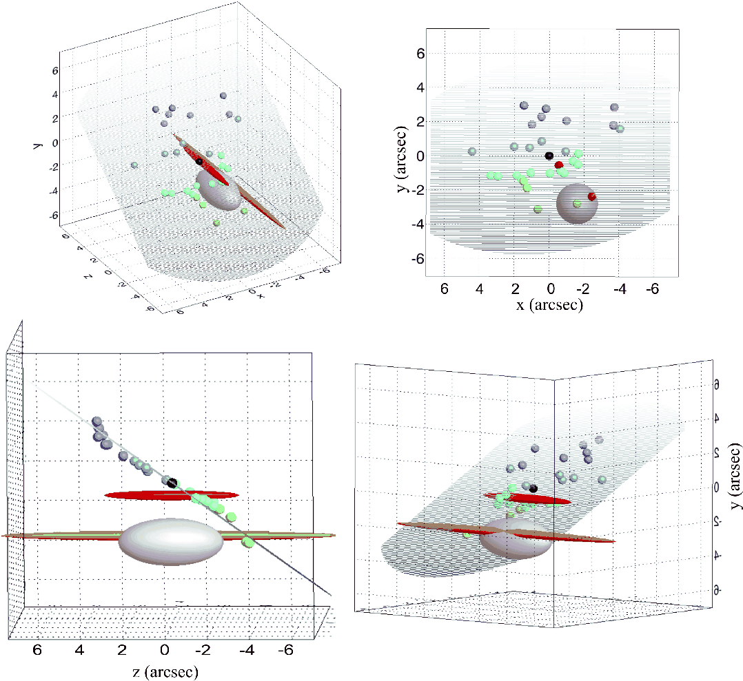
6 The 3D arrangement
Figure 6 shows a 3D reconstruction of some of the features found in the central parsec of the Galaxy. The shaded area represents the disk of clockwise-rotating stars (CWS, Paumard et al. 2006; Beloborodov et al. 2006; Lu et al. 2009), and the colored spheres are the stellar members. The positions of the stars and the disk parameters (nx, ny, nz)=(-0.12, -0.79, 0.6) are from Paumard et al. (2006). The stars are represented by different colors according to their distance from the observer (green is closer and violet is farther away from us).
Eckart et al. (2002)
show how a 3D separation r from the
center can be estimated by comparing the proper motion (
![]() )
of a star to the
3D velocity dispersion
)
of a star to the
3D velocity dispersion ![]() .
The probability that a star at the position rhas a
proper motion greater than
.
The probability that a star at the position rhas a
proper motion greater than ![]() can be calculated via
can be calculated via
The velocity dispersion
The mini-cavity is shown in pink: in projection we approximate
it with a circle of ![]() 1.2''
radius.
Paumard et al. (2004)
argue that the mini-cavity is a part of the Northern Arm of the
Mini-spiral. In
their reconstruction of the streamer 3D morphology, the mini-cavity
should be exactly in the plane
parallel to the plane of the sky and containing
Sgr A*, or be within
1.2''
radius.
Paumard et al. (2004)
argue that the mini-cavity is a part of the Northern Arm of the
Mini-spiral. In
their reconstruction of the streamer 3D morphology, the mini-cavity
should be exactly in the plane
parallel to the plane of the sky and containing
Sgr A*, or be within ![]() 2.5'' from it. This is in excellent agreement
with orbital
models of Zhao et al. (2009).
The
2.5'' from it. This is in excellent agreement
with orbital
models of Zhao et al. (2009).
The ![]() 2.5''
uncertainty of the line-of-sight position of the mini-cavity is
depicted as an elongation of the pink object in Fig. 6 along the z-axis.
2.5''
uncertainty of the line-of-sight position of the mini-cavity is
depicted as an elongation of the pink object in Fig. 6 along the z-axis.
|
Figure 6:
Three-dimensional view of some of the Galactic center features. The
axes show offsets
from Sgr A* (black sphere) in arcseconds. On the z-axis,
positive means farther away from the
observer than Sgr A*.
The shaded area represent the CWS disk and
the colored spheres stars belonging to it. The color scheme reflects
the distance from
the observer, with green closest and violet farthest away from us.
The bow shock sources are shown in red (X7) and orange (X3). Elongation
along
the z-axis reflects the uncertainty in the position
of the two sources along
the line of sight (see text). The pink spheroid represents the
mini-cavity: in projection
we plot it as a circle with radius |
| Open with DEXTER | |
7 Discussion
All the interesting physics that can result from the modeling
is contained in the equation for the bow shock standoff distance R0
(Eq. (3)).
The main drawback is a lack of knowledge about the stellar types (i.e.
stellar wind parameters)
of the two stars. The L'-band images are dominated
by the thermal emission of dust. Both X3 and X7 are bright
at 3.8![]() m, but
extremely faint at shorter wavelengths. Both features are apparently
not embedded in the
mini-spiral material, so we expect them to be intrinsically dusty.
m, but
extremely faint at shorter wavelengths. Both features are apparently
not embedded in the
mini-spiral material, so we expect them to be intrinsically dusty.
If there was no influence by any external wind, the bow shock
in our images would
point in the direction of the proper motion. We understand that the ![]() in Eqs. (2)
and (3) is
the relative velocity
between the stellar velocity vector and the external wind velocity
vector.
Since we do not have full 3D information about the stellar velocity,
but only
proper motions, the values of
in Eqs. (2)
and (3) is
the relative velocity
between the stellar velocity vector and the external wind velocity
vector.
Since we do not have full 3D information about the stellar velocity,
but only
proper motions, the values of ![]() that we calculate in the following represent lower limits for
the real external wind velocity.
For the orientation of the projected vector
that we calculate in the following represent lower limits for
the real external wind velocity.
For the orientation of the projected vector ![]() ,
we assume
the position angle PA of the bow-shock symmetry axis (Figs. 4 and 5).
By estimating
,
we assume
the position angle PA of the bow-shock symmetry axis (Figs. 4 and 5).
By estimating ![]() we can therefore determine the projected position of the external wind
source responsible for the observed bow-shock morphology.
we can therefore determine the projected position of the external wind
source responsible for the observed bow-shock morphology.
7.1 Nature of the source at the position of X7
In the following we discuss the possible nature of the X7 star, based
on its apparent brightness in the K-band (
![]() ), combined with the distance
modulus of 14.5
and extinction of
), combined with the distance
modulus of 14.5
and extinction of ![]() .
We discuss only stellar types that agree
with the K-band photometry.
.
We discuss only stellar types that agree
with the K-band photometry.
For the number density of the ambient medium we assume n = 26 cm-3
(Baganoff et al. 2003).
This value is reasonable since X7 is not moving through the denser
mini-spiral material.
- (1)
- Late B-type main sequence star (B7-8V).
For O and B galactic stars, the following relation holds:
where is in
is in  yr-1,
yr-1,
 in
km s-1,
in
km s-1,  in
in  ,
and
,
and  in
in
 (Lamers & Cassinelli 1999).
For a typical B7V star with
(Lamers & Cassinelli 1999).
For a typical B7V star with  and
and  ,
we then have
,
we then have
 yr-1 km s-1.
This kind of weak wind would require
yr-1 km s-1.
This kind of weak wind would require  of only 15 km s-1, a
negligible velocity
when compared to the proper motion of X7.
Also, B-type main sequence stars are dust-free objects and thus
probably
not good candidates for producing features like X7.
of only 15 km s-1, a
negligible velocity
when compared to the proper motion of X7.
Also, B-type main sequence stars are dust-free objects and thus
probably
not good candidates for producing features like X7.
- (2)
- Herbig Ae/Be (HAe/Be) star.
This class of intermediate-mass, pre-main sequence objects is
characterized by strong wind activity and infrared excess. Line
emission of
HAe/Be stars often shows prominent P-Cygni profiles, indicating
powerful
winds with mass-loss rates varying from 10-8 to
several times 10-6 yr-1,
and
wind velocities of several hundred km s-1
(e.g. Bouret
& Catala 1998; Benedettini et al. 1998;
Nisini
et al. 1995).
Nisini et al. (1995)
show that there is a correlation between mass-loss rate and bolometric
luminosity of HAe/Be stars. A star with
 would
have
would
have  yr-1.
Combined with
yr-1.
Combined with  km s-1,
this leads to
km s-1,
this leads to
 km s-1.
The external wind is then blowing with the velocity
km s-1.
The external wind is then blowing with the velocity
 km s-1
from the direction
km s-1
from the direction  60
60 (E of N).
We have to note that the
existence of the pre-main sequence stars at the GC is not established.
It is not yet clear
how the young (few Myr old) population in the central parsec has been
formed, since
the tidal field of Sgr A* prevents ``normal'' star formation
via
cloud collapse (e.g. Portegies Zwart
et al. 2006; Nayakshin 2006b). However,
the
possibility of YSO presence in the central parsec was discussed by Eckart et al. (2004)
and Muzic et al. (2008).
(E of N).
We have to note that the
existence of the pre-main sequence stars at the GC is not established.
It is not yet clear
how the young (few Myr old) population in the central parsec has been
formed, since
the tidal field of Sgr A* prevents ``normal'' star formation
via
cloud collapse (e.g. Portegies Zwart
et al. 2006; Nayakshin 2006b). However,
the
possibility of YSO presence in the central parsec was discussed by Eckart et al. (2004)
and Muzic et al. (2008).
- (3)
- Central stars of planetary nebulae (CSPN).
When all the hydrogen has been exhausted and the helium ignites in the
core of a low/intermediate mass star (1-8 ), the star
reaches the asymptotic giant branch (AGB).
A typical AGB star at the GC is 4 mag brighter in the K-band
than X7.
AGB stars experience high mass-loss rates that remove most of
the stellar envelope, leaving behind a stellar core. The star has now
entered the
post-AGB and then the planetary nebula (PN) phase. During this phase
the central star remains at constant luminosity, while
 rises; i.e., the star moves towards the left side of the HR diagram in
a
horizontal line. CSPN are characterized by small mass losses, but very
fast
stellar winds.
A typical CSPN with
rises; i.e., the star moves towards the left side of the HR diagram in
a
horizontal line. CSPN are characterized by small mass losses, but very
fast
stellar winds.
A typical CSPN with  yr-1,
yr-1,
 km s-1,
and
km s-1,
and  (Lamers & Cassinelli 1999)
will have
(Lamers & Cassinelli 1999)
will have
 ,
therefore
,
therefore  for
for  -4.8).
The evolution of a star from the AGB phase towards
the final white dwarf stage is rapid (e.g. Blöcker
1995), and the star
will remain at the required brightness for less than 1000 yr
before it
becomes too faint. By adopting the typical CSPN parameters,
we obtain
-4.8).
The evolution of a star from the AGB phase towards
the final white dwarf stage is rapid (e.g. Blöcker
1995), and the star
will remain at the required brightness for less than 1000 yr
before it
becomes too faint. By adopting the typical CSPN parameters,
we obtain  km s-1,
and
km s-1,
and
 km s-1
from the direction 62
(E of N).
km s-1
from the direction 62
(E of N).
- (4)
- Low-luminosity Wolf-Rayet (WR) star; [WC]-type star.
Population I WR stars are massive stars in a late stage of evolution.
With typical luminosities between
 and 106 ,
they
are several magnitudes brighter than X7, unless the local extinction
at the position of X7 is much higher than the estimated value of AK=2.5.
A class of CSPNe identified as WR stars share the origin with other PNe
stars, but
are spectroscopically classified as WR stars because emission-line
spectra
for both types of objects come from expanding H-poor stellar winds. WR
stars in PNe almost
exclusively appear to be of the WC type (e.g. Gorny
et al. 1995), and are labeled as [WC].
About 15
and 106 ,
they
are several magnitudes brighter than X7, unless the local extinction
at the position of X7 is much higher than the estimated value of AK=2.5.
A class of CSPNe identified as WR stars share the origin with other PNe
stars, but
are spectroscopically classified as WR stars because emission-line
spectra
for both types of objects come from expanding H-poor stellar winds. WR
stars in PNe almost
exclusively appear to be of the WC type (e.g. Gorny
et al. 1995), and are labeled as [WC].
About 15 of all the observed CSPNe appear to be [WC] (Acker
& Neiner 2003).
PNe stars with WR stars in their centers have, in general, larger
infrared excess than normal
CSPNe (Kwok 2000) and more
powerful winds. Crowther (2008)
reviewed the properties
of [WC] stars. Typically, winds are characterized by
-10-6 yr-1
and
of all the observed CSPNe appear to be [WC] (Acker
& Neiner 2003).
PNe stars with WR stars in their centers have, in general, larger
infrared excess than normal
CSPNe (Kwok 2000) and more
powerful winds. Crowther (2008)
reviewed the properties
of [WC] stars. Typically, winds are characterized by
-10-6 yr-1
and  -2000 km s-1.
Adopting the lower limit values for
and ,
we obtain
-2000 km s-1.
Adopting the lower limit values for
and ,
we obtain
 km s-1,
 km s-1
from the direction 65
(E of N).
For the average values
km s-1
from the direction 65
(E of N).
For the average values  and
and  km s-1,
we have
km s-1,
we have  km s-1,
 km s-1
from the direction 55
(E of N).
km s-1
from the direction 55
(E of N).
7.2 Nature of the source at the position of X3
In contrast to X7, there is no detectable point source at the
position of X3 in our ![]() -band
images. Crowding makes individual stars
of
-band
images. Crowding makes individual stars
of ![]() difficult to detect within the central parsec,
so we define this value as an upper limit on the brightness of X3 in
the K-band.
Here we discuss the possible nature of the star at the position of X3,
and
give possible solutions for the external wind direction and velocity.
difficult to detect within the central parsec,
so we define this value as an upper limit on the brightness of X3 in
the K-band.
Here we discuss the possible nature of the star at the position of X3,
and
give possible solutions for the external wind direction and velocity.
- (1)
- Main sequence star.
If on the main sequence, a star with
 would be of type A0 or later.
The mass-loss rate of
low-mass stars during the core H-burning phase is
very low, in the range 10-12-10-10 yr-1(Lamers & Cassinelli 1999).
In this case, any ISM streaming with the velocity on the order of
10 km s-1 could produce the
bow shock with
the standoff distance of X3. As in the case of X7, a
main sequence star cannot be a source of a dust-rich envelope
observed in the L'-band, so we can rule out the
main sequence
nature of X3.
would be of type A0 or later.
The mass-loss rate of
low-mass stars during the core H-burning phase is
very low, in the range 10-12-10-10 yr-1(Lamers & Cassinelli 1999).
In this case, any ISM streaming with the velocity on the order of
10 km s-1 could produce the
bow shock with
the standoff distance of X3. As in the case of X7, a
main sequence star cannot be a source of a dust-rich envelope
observed in the L'-band, so we can rule out the
main sequence
nature of X3.
- (2)
- CSPN or [WC]-type star.
As a CSPN evolves on the horizontal track in the HR diagram, it
maintains
the same luminosity while increasing the effective temperature. The
peak emission
of the stellar black body shifts bluewards and the star becomes fainter
in
the infrared. A typical CSPN or [WC]-star discussed above for X7 would
have mK>18
for
 .
Adopting the typical CSPN parameters,
we obtain
.
Adopting the typical CSPN parameters,
we obtain  km s-1
and
km s-1
and
 km s-1
from the direction 61
(E of N).
For [WR]-star, using lower limit values as above, we obtain
km s-1
from the direction 61
(E of N).
For [WR]-star, using lower limit values as above, we obtain  km s-1,
and
km s-1,
and  km s-1
from
the direction 62
(E of N).
km s-1
from
the direction 62
(E of N).
- (3)
- Dust blob. Since with the current sensitivity of our observations we do not detect a point source in the K-band, we cannot rule out the possibility that X3 is a dust blob ablated by a wind from the direction of Sgr A*, rather than a stellar source. This scenario could explain the observed elongated tail. The proper motion suggests that the feature moves along with the rest of the material in the IRS13 region. In this case modeling the feature as a bow shock is superfluous.
7.3 Nature of the external wind
The first question that to ask is about a wind source
that can drive a shock of a certain velocity over a distance of few
tenths of parsec.
The argument of the ram pressure of such a wind at the given
distance d leads to

where
The number of PNe expected to reside within the central parsec
can be estimated as
|
(9) |
where N*(m) stands for the number of stars of the mass m currently present in the GC population,
The alignment of the two features is still not explained. In
the case of an
isotropic wind arising from the mass-losing stars, one would expect
a more random distribution of such sources around the center.
Curiously, the two sources are arranged in the exact direction
in which the mini-cavity is projected onto the sky.
If we do not think of this arrangement as a chance configuration, this
might indicate that
(i) all three features (X3, X7, and the mini-cavity)
are produced by the same
event, and (ii) there is a preferred direction in
which the mass
is expelled at the GC. The possibility of a collimated outflow was
already
discussed by Muzic et al.
(2007). This outflow could also account for narrow
dust filaments of the Northern Arm of the mini-spiral, as well
as the H2-bright lobes of the circumnuclear disk
(CND). As
the authors argue, the outflow could be linked to the
plane of the mass-losing stars so that the matter
provided by stars and not accreted onto Sgr A* is expelled
perpendicular to the plane. Having an opening angle of about 30![]() ,
this
outflow could account for the mini-cavity, X3, and X7 at the same time.
In this case X3 and X7 should be located not too far away from the
plane
containing Sgr A*, which is already suggested by the high
inclination (
,
this
outflow could account for the mini-cavity, X3, and X7 at the same time.
In this case X3 and X7 should be located not too far away from the
plane
containing Sgr A*, which is already suggested by the high
inclination (
![]() )
of the two bow shocks to the line of sight resulting from our modeling.
)
of the two bow shocks to the line of sight resulting from our modeling.
8 Summary and conclusions
We have presented L'-band observations of the two
comet-shaped sources in the vicinity of Sgr A*, named X3 and
X7.
The symmetry axes of the two sources are aligned within 5![]() in the
plane of the sky
and the tips of their bow shocks point towards Sgr A*. Our
measurements show that
the proper motion vectors of both features are pointing in directions
more than
45
in the
plane of the sky
and the tips of their bow shocks point towards Sgr A*. Our
measurements show that
the proper motion vectors of both features are pointing in directions
more than
45![]() away from the line that connects them with Sgr A*.
Proper motion velocities are high, at several 100 km s-1.
This misalignment of the bow-shock
symmetry axes and their proper motion vectors, together with
high proper motions, suggest that the bow-shocks must
be produced by an interaction with some external strong wind, possibly
coming from
Sgr A* or stars in its vicinity.
away from the line that connects them with Sgr A*.
Proper motion velocities are high, at several 100 km s-1.
This misalignment of the bow-shock
symmetry axes and their proper motion vectors, together with
high proper motions, suggest that the bow-shocks must
be produced by an interaction with some external strong wind, possibly
coming from
Sgr A* or stars in its vicinity.
We developed a bow-shock model to fit the observed morphology and constrain the source of the external wind. The stellar types of the two stars are not known. Moreover, one of the features is likely not a star, but just a dust structure. It might be located at the edge of the mini-cavity, and shaped by the same wind that produces the X7 bow shock.
We discussed the nature of the external wind and showed that neither one of the features can arise via interaction with an external wind coming from a single, mass-losing star. Instead, the observed properties of the bow shocks provide evidence for interaction with a fast and strong wind produced probably by an ensemble of mass-losing sources. Alternatively, a possible source of the wind could be Sgr A*. Shock velocities that can result from such a combined outflow over a distance assumed for the two features X3 and X7, match the velocities required to produce the bow shocks of stars in the late evolution stages of CSPNe or [WC]-stars. Short lifetimes of such stars can explain the lack of other similar comet-shaped sources in the central parsec.
We discuss our results in the light of the
partially-collimated outflow
already proposed in Muzic
et al. (2007) and argue that
such an outflow, arising perpendicular to the CWS, can account for X3
and X7, as
well as for the mini-cavity.
The collective wind from the CWS has a scale of ![]() 10 arcsec.
On scales of about an arcsecond or less theoretical studies
predict a radius-dependent accretion flow (e.g. Yuan et al. 2003; Blandford
& Begelman 1999).
Within this region the flow of a major portion of the material
originally bound for accretion onto Sgr A* is inverted and the
material is expelled again towards larger radii.
The presence of a strong outbound wind
at projected distances from Sgr A* of only 0.8" (X7) with a
mass load of 10-3
10 arcsec.
On scales of about an arcsecond or less theoretical studies
predict a radius-dependent accretion flow (e.g. Yuan et al. 2003; Blandford
& Begelman 1999).
Within this region the flow of a major portion of the material
originally bound for accretion onto Sgr A* is inverted and the
material is expelled again towards larger radii.
The presence of a strong outbound wind
at projected distances from Sgr A* of only 0.8" (X7) with a
mass load of 10-3 ![]() yr-1
does in fact agree with models that predict a highly inefficient
accretion onto the central BH owing to a strongly radius dependent
accretion flow.
yr-1
does in fact agree with models that predict a highly inefficient
accretion onto the central BH owing to a strongly radius dependent
accretion flow.
Knowledge of wind parameters for two bow-shock stars is crucial for drawing more quantitative conclusions on the nature of the external outflow. Spectroscopy should therefore be the next step to confirm our hypothesis.
AcknowledgementsThe authors would like to thank the referee, Dr. Mark Morris, for valuable comments and suggestions that helped to improve this work. Part of this work was supported by the Deutsche Forschungsgemeinschaft (DFG) via SFB 494. R.S. acknowledges the Ramón y Cajal program of the Spanish Ministerio de Ciencia e Innovación. M.Z. was supported for this research through a stipend from the International Max Planck Research School (IMPRS) for Astronomy and Astrophysics at the Universities of Bonn and Cologne.
References
- Acker, A., & Neiner, C. 2003, A&A, 403, 659 [NASA ADS] [CrossRef] [EDP Sciences] [Google Scholar]
- Baganoff, F. K., Maeda, Y., Morris, M., et al. 2003, ApJ, 591, 891 [NASA ADS] [CrossRef] [Google Scholar]
- Beloborodov, A. M., Levin, Y., Eisenhauer, F., et al. 2006, ApJ, 648, 405 [NASA ADS] [CrossRef] [Google Scholar]
- Benedettini, M., Nisini, B., Giannini, T., et al. 1998, A&A, 339, 159 [NASA ADS] [Google Scholar]
- Blandford, R., & Begelman, M. 1999, MNRAS, 303, L1 [NASA ADS] [CrossRef] [Google Scholar]
- Blöcker, T. 1995, A&A, 299, 755 [NASA ADS] [Google Scholar]
- Bouret, J.-C., & Catala, C. 1998, A&A, 340, 163 [NASA ADS] [Google Scholar]
- Bower, G. C., Wright, M. C. H., Falcke, H., & Backer, D. C. 2003, ApJ, 588, 331 [NASA ADS] [CrossRef] [Google Scholar]
- Brandner, W., Rousset, G., Lenzen, R., et al. 2002, Messenger, 107, 1 [Google Scholar]
- Comerón, F., & Kaper, L. 1998, A&A, 338, 273 [NASA ADS] [Google Scholar]
- Crowther, P. A. 2008, in Hydrogen-Deficient Stars, ed. K. Werner, & T. Rauch, ASP Conf. Ser., 391, 83 [Google Scholar]
- Eckart, A., & Duhoux, P. R. M. 1990, in Astrophysics with Infrared Arrays, ed. R. Elston (San Francisco: ASP), ASP Conf. Ser., 14, 336 [Google Scholar]
- Eckart, A., Genzel, R., Krabbe, A., et al. 1992, Nature, 355, 526 [NASA ADS] [CrossRef] [Google Scholar]
- Eckart, A., Genzel, R., Ott, T., & Schödel, R. 2002, MNRAS, 331, 917 [NASA ADS] [CrossRef] [Google Scholar]
- Eckart, A., Moultaka, J., Viehmann, T., Straubmeier, C., & Mouawad, N. 2004, ApJ, 602, 760 [CrossRef] [Google Scholar]
- Eisenhauer, F., Genzel, R., Alexander, T., et al. 2005, ApJ, 628, 246 [NASA ADS] [CrossRef] [Google Scholar]
- Figer, D. F., Sungsoo, K., Morris, M., et al. 1999, ApJ, 525, 750 [NASA ADS] [CrossRef] [Google Scholar]
- Figer, D. F., Rich, M., Sungsoo, K., Morris, M., & Serabyn, E. 2004, ApJ, 601, 319 [NASA ADS] [CrossRef] [Google Scholar]
- Ghez, A. M., Salim, S., Hornstein, S. D., et al. 2005, ApJ, 620, 744 [NASA ADS] [CrossRef] [Google Scholar]
- Ghez, A. M., Salim, S., Weinberg, N. N., et al. 2008, ApJ, 689, 1044 [NASA ADS] [CrossRef] [Google Scholar]
- Gillessen, S., Eisenhauer, F., Trippe, S., et al. 2009, ApJ, 692, 1075 [NASA ADS] [CrossRef] [Google Scholar]
- Gorny, S. K., Acker, A., Stasinska, G., Stenholm, B., & Tylenda, R. 1995, in Proc. IAU Symp. 163, ed. K. A. van der Hucht, & P. M. Williams, 85 [Google Scholar]
- Krügel, E. 2003, The Physics of Interstellar Dust (IOP Publishing), Series in Astronomy and Astrophysics [Google Scholar]
- Kwok, S. 2000, The Origin and Evolution of Planetary Nebulae (Cambridge University Press) [Google Scholar]
- Lamers, H. J. G. L. M., & Cassinelli, J. P. 1999, Introduction to Stellar Winds (Cambridge University Press) [Google Scholar]
- Laor, A., & Draine, B. T. 1993, ApJ, 402, 441 [NASA ADS] [CrossRef] [Google Scholar]
- Lenzen, R., Hofmann, R., Bizenberger, P., & Tusche, A. 1998, in Infrared Astronomical Instrumentation, ed. A. M. Fowler, Proc. SPIE, 3354, 606 [Google Scholar]
- Lu, J. R., Ghez, A. M., Hornstein, S. D., et al. 2009, ApJ, 690, 1463 [NASA ADS] [CrossRef] [Google Scholar]
- Lutz, D., Krabbe, A., & Genzel, R. 1993, ApJ, 418, 244 [NASA ADS] [CrossRef] [Google Scholar]
- Mac Low, M. M., van Buren, D., Wood, D. O. S., & Churchwell, E. 1991, ApJ, 369, 395 [NASA ADS] [CrossRef] [Google Scholar]
- Marrone, D. P., Moran, J. M., Zhao, J.-H., & Rao, R. 2006, ApJ, 640, 308 [NASA ADS] [CrossRef] [Google Scholar]
- Mathis, J. S., Rumpl, W., & Nordsieck, K. H. 1977, ApJ, 217, 425 [NASA ADS] [CrossRef] [Google Scholar]
- Muzic, K., Eckart, A., Schödel, R., Meyer, L., & Zensus, A. 2007, A&A, 469, 993 [NASA ADS] [CrossRef] [EDP Sciences] [Google Scholar]
- Muzic, K., Schödel, R., Eckart, A., Meyer, L., & Zensus, A. 2008, A&A, 482, 173 [NASA ADS] [CrossRef] [EDP Sciences] [Google Scholar]
- Najarro, F., Krabbe, A., Genzel, R., et al. 1997, A&A, 325, 700 [NASA ADS] [Google Scholar]
- Nayakshin, S. 2006b, in J. Phys. Conf. Ser. 54, ed. R. Schödel, G. C. Bower, M. P. Muno, S. Nayakshin, & T. Ott, 208 [Google Scholar]
- Nisini, B., Milillo, A., Saraceno, P., & Vitali, F. 1995, A&A, 302, 169 [NASA ADS] [Google Scholar]
- Paumard, T., Maillard, J.-P., & Morris, M. 2004, A&A, 426, 81 [NASA ADS] [CrossRef] [EDP Sciences] [Google Scholar]
- Paumard, T., Genzel, R., Martins, F., et al. 2006, ApJ, 643, 1011 [NASA ADS] [CrossRef] [Google Scholar]
- Portegies Zwart, S. F., Baumgardt, H., McMillan, S. L. W., et al. 2006, ApJ, 641, 319 [NASA ADS] [CrossRef] [Google Scholar]
- Povich, M. S., Benjamin, R. A., Whitney, B. A., et al. 2008, ApJ, 689, 242 [NASA ADS] [CrossRef] [Google Scholar]
- Raga, A. C., Noriega-Crespo, A., Cantó, J., et al. 1997, RMxAA, 33, 73 [Google Scholar]
- Rousset, G., Lacombe, F., Puget, P., et al. 1998, in Adaptive Optical System Technologies, ed. D. Bonaccini, Proc. SPIE, 3353, 516 [Google Scholar]
- Schödel, R., Ott, T., Genzel, R., et al. 2003, ApJ, 596, 1015 [NASA ADS] [CrossRef] [Google Scholar]
- Schödel, R., Eckart, A., Alexander, T., et al. 2007, A&A, 469, 125 [NASA ADS] [CrossRef] [EDP Sciences] [Google Scholar]
- Schödel, R., Najarro, F., Muzic, K., & Eckart, A. 2010, A&A, 511, A18 [NASA ADS] [CrossRef] [EDP Sciences] [Google Scholar]
- Tanner, A., Ghez, A. M., Morris, M. R., & Christou, J. C. 2005, ApJ, 624, 742 [NASA ADS] [CrossRef] [Google Scholar]
- Van Buren, D., & McCray, R. 1988, ApJ, 329, L93 [NASA ADS] [CrossRef] [Google Scholar]
- Villaver, E., Manchado, A., & García-Segura, G. 2002, ApJ, 581, 1204 [NASA ADS] [CrossRef] [Google Scholar]
- Wilkin, F. P. 1996, Models of Interacting Stellar Winds, Ph.D. Thesis, University of California, Berkley [Google Scholar]
- Yuan, F., Quataert, E., & Narayan, R. 2003, ApJ, 598, 301 [NASA ADS] [CrossRef] [Google Scholar]
- Yusef-Zadeh, F., & Melia, F. 1992, Ap, 385, L41 [Google Scholar]
- Yusef-Zadeh, F., & Wardle, M. 1993, ApJ, 405, 584 [NASA ADS] [CrossRef] [Google Scholar]
- Yusef-Zadeh, F., Morris, M., & Ekers, R. D. 1990, Nature, 348, 45 [NASA ADS] [CrossRef] [Google Scholar]
- Zhang, Q., & Zheng, X. 1997, ApJ, 474, 719 [NASA ADS] [CrossRef] [Google Scholar]
- Zhao, J.-H., Morris, M. R., Goss, W. M., & An, T. 2009, ApJ, 699, 186 [NASA ADS] [CrossRef] [Google Scholar]
Footnotes
- ...
![[*]](/icons/foot_motif.png)
- Present address: Department of Astronomy and Astrophysics, University of Toronto, 50 St. George Street, Toronto ON M5S 3H4, Canada.
- ...(Laor & Draine 1993)
- Available at http://www.astro.princeton.edu/~draine/
All Figures
|
|
Figure 1:
NACO L'-band (3.8 |
| Open with DEXTER | |
| In the text | |
|
|
Figure 2:
L'-band proper motions of the two comet-shaped
features X3 and X7. The error bars show the 1 |
| Open with DEXTER | |
| In the text | |
|
|
Figure 3:
The 2D bow-shock shape.
Full line shows the analytic model from Wilkin
(1996, see Eq. (1). Dotted
lines show narrow solutions (Zhang
& Zheng 1997), for two collimation angles |
| Open with DEXTER | |
| In the text | |
|
|
Figure 4:
Results of our modeling for the feature X7 (black contours), observed
in the epoch 2003.36. The image is previously deconvolved and
beam-restored to the nominal resolution of our L'-band
images. Color contours represent the bow-shock model projected onto
the plane of the sky.
|
| Open with DEXTER | |
| In the text | |
|
|
Figure 5:
Best-fit results of the modeling for the feature X3 (black contours)
observed in the epoch 2003.36. The image is previously deconvolved and
beam-restored to the nominal resolution of our L'-band
images. Color contours represent the bow-shock model projected onto
the plane of the sky.
|
| Open with DEXTER | |
| In the text | |
|
|
Figure 6:
Three-dimensional view of some of the Galactic center features. The
axes show offsets
from Sgr A* (black sphere) in arcseconds. On the z-axis,
positive means farther away from the
observer than Sgr A*.
The shaded area represent the CWS disk and
the colored spheres stars belonging to it. The color scheme reflects
the distance from
the observer, with green closest and violet farthest away from us.
The bow shock sources are shown in red (X7) and orange (X3). Elongation
along
the z-axis reflects the uncertainty in the position
of the two sources along
the line of sight (see text). The pink spheroid represents the
mini-cavity: in projection
we plot it as a circle with radius |
| Open with DEXTER | |
| In the text | |
Copyright ESO 2010
Current usage metrics show cumulative count of Article Views (full-text article views including HTML views, PDF and ePub downloads, according to the available data) and Abstracts Views on Vision4Press platform.
Data correspond to usage on the plateform after 2015. The current usage metrics is available 48-96 hours after online publication and is updated daily on week days.
Initial download of the metrics may take a while.