| Issue |
A&A
Volume 520, September-October 2010
|
|
|---|---|---|
| Article Number | A63 | |
| Number of page(s) | 4 | |
| Section | Numerical methods and codes | |
| DOI | https://doi.org/10.1051/0004-6361/201015278 | |
| Published online | 04 October 2010 | |
New uniform grids on the sphere
D. Rosca
Technical University of Cluj-Napoca, Department of mathematics, str. Memorandumului 28, 400114 Cluj-Napoca, Romania
Received 24 June 2010 / Accepted 17 July 2010
Abstract
Aims. A method for constructing new uniform grids on the sphere is given.
Methods. We define a bijection in
![]() ,
which maps squares onto discs and preserves areas. Then we use this
bijection, combined with Lambert azimuthal projection, for lifting
uniform grids from the square to the sphere.
,
which maps squares onto discs and preserves areas. Then we use this
bijection, combined with Lambert azimuthal projection, for lifting
uniform grids from the square to the sphere.
Results. We can obtain uniform spherical grids that allow a
hierarchical data manipulation and have an isolatitudinal distribution
of cells. Compared with HEALPix grids, nowadays the most used in
astronomy and astrophysics, our grids have the advantage of allowing
easier implementation, and in addition one can move approximating
functions from the square to the sphere by a simple technique.
Key words: miscellaneous - methods: data analysis - methods: numerical - methods: statistical
1 Introduction
The analysis of functions defined on spherical domains plays a central role in geosciences. In many applications, one needs uniform grids on the sphere. The standard manipulation of spherical data includes convolutions with local and global kernels, Fourier analysis with spherical harmonics, wavelet analysis, nearest neighbour search, etc. Some of these manipulations become very slow if the sampling of functions on the sphere and the related discrete data set are not designed well. Thus, the discrete data should have the following properties: (a) hierarchical tree structure (allowing construction of a multiresolution analysis); (b) equal area for the discrete elements of the partition of the sphere; (c) isolatitudinal distribution for the discrete area elements (essential for fast computations involving spherical harmonics).
There are plenty of spherical grids and sampling points, many of them mentioned in Gorsky et al. (2005). A complete description of all known spherical projections used in cartography is realized in (Grafarend & Krumm 2006; Snyder 1993).
Until the construction of the HEALPix grid, no grid satisfied
simultaneous the requirements (a)-(c). In this paper we give
a method for constructing uniform grids and sampling points on the
2-sphere, satisfying these requirements simultaneously. We start with a
bijection on
![]() ,
which preserves areas and maps a square in a disc. Thus, any
uniform grid of the square can be mapped bijectively onto a uniform
grid on the disc, and then onto a uniform grid on the sphere, via
Lambert's equal area azimuthal projection. Compared to the projections
used for HEALPix grids and to the planar domains mapped there, our
method has the nice property that, besides the uniform grids and
sampling points on the sphere, one can transport any function from the square to the sphere by the technique used in Rosca & Antoine (2009).
In addition, if we have a set of real functions defined on
the square, the corresponding spherical functions preserve the
following properties: orthonormal basis, Riesz basis, frame, and local
support.
,
which preserves areas and maps a square in a disc. Thus, any
uniform grid of the square can be mapped bijectively onto a uniform
grid on the disc, and then onto a uniform grid on the sphere, via
Lambert's equal area azimuthal projection. Compared to the projections
used for HEALPix grids and to the planar domains mapped there, our
method has the nice property that, besides the uniform grids and
sampling points on the sphere, one can transport any function from the square to the sphere by the technique used in Rosca & Antoine (2009).
In addition, if we have a set of real functions defined on
the square, the corresponding spherical functions preserve the
following properties: orthonormal basis, Riesz basis, frame, and local
support.
Consider the square of edge 2L and the circle with the same area, both centred on the origin O (Fig. 1). The radius of the circle will be
![]() We want to construct a bijection T from the domain
We want to construct a bijection T from the domain

to the disc of radius R,

such that
Here
The first idea is to construct a map by keeping the direction of the position vector, that is, for ![]() to take T(M) on the half-line OM. If we define such an application which maps the square
to take T(M) on the half-line OM. If we define such an application which maps the square

into the circle

for every
Therefore, an alternative would be to take a rotation around O,
followed by an appropriate move along the radius. This construction is
described bellow. We focus for the moment on the first octant I of the plane, intersected with the square SL,

The map T will be defined in such a way that each half-line

In this way, the half lines y=0 and y=x, situated on the boundary of I are invariant under T and
The point Q will be mapped on the point P(X,Y), the intersection of the half-line dk(m) with the circle

Therefore, the point P has the coordinates

We define N=T(M) such that

Straightforward calculations show that the Jacobian of the map T, restricted to I, is indeed 1, and therefore T preserves the areas of the domains situated in the first octant I.
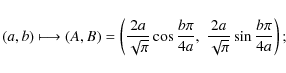
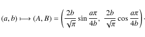
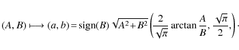
By similar arguments for the seven other octants, we find that the map
![]() preserving areas is defined as follows:
preserving areas is defined as follows:
- 1.
- For
 ,
,
- 2.
- For

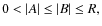
The inverse of T is given by the following formulas:
- 1.
- For
 ,
,
- 2.
- For
![\begin{figure}
\par\includegraphics[width=6cm,clip]{15278fig1.eps}
\end{figure}](/articles/aa/full_html/2010/12/aa15278-10/img37.png)
|
Figure 1: The action of the transform T. Points N and P are the images of M and Q, respectively. |
| Open with DEXTER | |
| Figure 2: A horizontal grid and its image grid on the disc. The image of the bold line on the left is the bold curve on the right. |
|
| Open with DEXTER | |
| Figure 3: Two uniform grids of the disc, where the right one is the refinement of the left one. |
|
| Open with DEXTER | |
2 Spherical grids
We intend to use our transform to construct uniform grids on the sphere. In a uniform grid, all the cells have the same area. The idea is to start from a uniform grid on a square, first to map it onto a disc using the map T and then use an equal area projection from the disc to the sphere. An example of such a projection is Lambert's azimuthal projection.
2.1 Lambert's azimuthal equal area projection
This projection was constructed in 1772 by J. H. Lambert, and it is the most used projection in cartography for mapping one hemisphere of the Earth onto a disc. This projection establishes a bijection between a sphere of radius r, without a point, and the interior of a disc of radius 2r and it preserves areas. To define the Lambert azimuthal projection (see Fig. 4), we need the plane tangent to the sphere at some point S on the sphere. Let P be an arbitrary point on the sphere other than the antipode of S. Let d be the Euclidean distance between S and P (not the distance along the sphere surface). The projection of P will be the point P' on the plane, such that SP'=d. Geometrically, it can be constructed as follows. We consider the unique circle centred on S, passing through P and perpendicular to the plane. This circle intersects the plane at two points and we take P' those point that is closer to P. This is the projected point (Fig. 4). The antipode of S is excluded from the projection because the required circle is not unique. The projection of S is taken as S.
| Figure 4: Lambert azimuthal projection. |
|
| Open with DEXTER | |
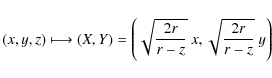
If we take the sphere
![]() of equation
x2+y2+z2=r2 and S(0,0,-r)
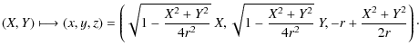
the south pole, then Lambert's projection and its inverse can be
described, in Cartesian coordinates, by the following formulas:
of equation
x2+y2+z2=r2 and S(0,0,-r)
the south pole, then Lambert's projection and its inverse can be
described, in Cartesian coordinates, by the following formulas:
and
2.2 Spherical uniform grids using Lambert's azimuthal projection for the whole sphere
We want to construct a uniform grid on the sphere
![]() starting from a uniform grid of the square
starting from a uniform grid of the square
![]() of edge
of edge
![]() .
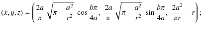
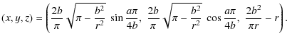
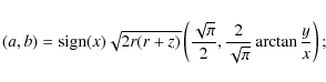
By combining the formulas (7) and (2), (3), we obtain that a point
.
By combining the formulas (7) and (2), (3), we obtain that a point
![]() is mapped into the point
is mapped into the point
![]() with the following coordinates:
with the following coordinates:
- 1.
- For
,
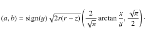
- 2.
- For
- 1.
- For
 ,
,
- 2.
- For

| Figure 5: The grids in Fig. 3, projected on the sphere by Lambert's projection. |
|
| Open with DEXTER | |
Two examples of such spherical uniform grids are given in Fig. 5. One can see that, because of the Lambert projection, the distortion of shape increases towards the north pole. For this reason, one can construct another type of spherical grids, by applying the Lambert projection separately for the two hemispheres.
2.3 Spherical grid using Lambert's azimuthal projection for each of the hemispheres
When we use Lambert's projection, we can choose to map only the
southern hemisphere with respect to the south pole, and separately, the
northern hemisphere with respect to the north pole. If the sphere
has the radius r, then the projected discs of each hemisphere have the radius ![]() and therefore the corresponding square will be
and therefore the corresponding square will be
![]() of edge
of edge
![]() .
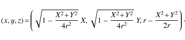
The formula for the spherical image (x,y,z) of a point (X,Y) of the disc
.
The formula for the spherical image (x,y,z) of a point (X,Y) of the disc
![]() are the one given in (7) for (x,y,z) in the southern hemisphere, while for the northern hemisphere it is given by
are the one given in (7) for (x,y,z) in the southern hemisphere, while for the northern hemisphere it is given by
For the inverse projection, a point (x,y,z) on the southern hemisphere projects according to formula (6), while for a point (x,y,z) on the northern hemisphere, the projection onto the disc
Similarly, formulas (8), (9) are the ones used for the points (x,y,z) on the southern hemisphere, while for the northern hemisphere, only the sign of z changes in both of these formulas. As for the images in the square
| Figure 6: The grids in Fig. 3, projected on the sphere by Lambert's projection, separately for the northern and southern hemispheres. |
|
| Open with DEXTER | |
The number of cells at each latitude for the square grid
We focus on the spherical grid with 8n2 cells, for which the grid on each hemisphere is the image of a uniform grid of the square [-L,L], with
![]() .
On this square we consider the grid containing (2n)2
small squares of the same area, formed by lines parallel to the edges.
The centres of the cells of the spherical grid are equally distributed
on 2n latitudinal circles, symmetric with respect to the
equator. The latitudinal circles are, in fact, images of squares
centred on O. The number of cells in the northern hemisphere (and of course, symmetric on the southern hemisphere) will be 4(2i-1) on the ith latitudinal circle.
.
On this square we consider the grid containing (2n)2
small squares of the same area, formed by lines parallel to the edges.
The centres of the cells of the spherical grid are equally distributed
on 2n latitudinal circles, symmetric with respect to the
equator. The latitudinal circles are, in fact, images of squares
centred on O. The number of cells in the northern hemisphere (and of course, symmetric on the southern hemisphere) will be 4(2i-1) on the ith latitudinal circle.
3 Conclusions
The equal area projection that maps squares onto circles (to the best of our knowledge this projection has not been constructed before) allowed us to construct uniform grids on a disc and on a sphere. We presented here only the pictures for the spherical grid generated by a square grid with square cells, but of course there are many other uniform grids on the square, which can be mapped to nice uniform grids on the sphere.
There are still many open questions. Do the centers of some spherical grid cells constitute fundamental systems of points? How do cubature formulas with such points behave? Which wavelets on the interval can be efficiently mapped on the sphere? How efficient are the new grids for geo-statistical applications? In which applications are our grids preferable to other grids? These will be the subjects of future work.
This work is supported by the grant POSDRU/89/ 1.5/S/62557, funded by the European Social Fund.
References
- Gorski, K. M., Hivon, E., Banday, A. J., et al. 2005, ApJ, 622, 759 [NASA ADS] [CrossRef] [Google Scholar]
- Grafarend, E. W., & Krumm, F. W. 2006, Map Projections (Berlin-Heidelberg: Springer Verlag) [Google Scholar]
- Rosca, D., & Antoine, J. P. 2009, Math. Probl. Eng [Google Scholar]
- Snyder, J. P. 1993, Flattening the Earth (Chicago and London: University of Chicago Press) [Google Scholar]
All Figures
|
|
Figure 1: The action of the transform T. Points N and P are the images of M and Q, respectively. |
| Open with DEXTER | |
| In the text | |
| |
Figure 2: A horizontal grid and its image grid on the disc. The image of the bold line on the left is the bold curve on the right. |
| Open with DEXTER | |
| In the text | |
| |
Figure 3: Two uniform grids of the disc, where the right one is the refinement of the left one. |
| Open with DEXTER | |
| In the text | |
| |
Figure 4: Lambert azimuthal projection. |
| Open with DEXTER | |
| In the text | |
| |
Figure 5: The grids in Fig. 3, projected on the sphere by Lambert's projection. |
| Open with DEXTER | |
| In the text | |
| |
Figure 6: The grids in Fig. 3, projected on the sphere by Lambert's projection, separately for the northern and southern hemispheres. |
| Open with DEXTER | |
| In the text | |
Copyright ESO 2010
Current usage metrics show cumulative count of Article Views (full-text article views including HTML views, PDF and ePub downloads, according to the available data) and Abstracts Views on Vision4Press platform.
Data correspond to usage on the plateform after 2015. The current usage metrics is available 48-96 hours after online publication and is updated daily on week days.
Initial download of the metrics may take a while.