Demonstration of exoplanet detection using an infrared telescope array

S. R. Martin; A. J. Booth

doi:10.1051/0004-6361/201014942

Home

All issues

Volume 520 (September-October 2010)

A&A, 520 (2010) A96

Full HTML

Free Access

Issue		A&A Volume 520, September-October 2010


Article Number		A96
Number of page(s)		16
Section		Astronomical instrumentation
DOI		https://doi.org/10.1051/0004-6361/201014942
Published online		08 October 2010

A&A 520, A96 (2010)

Demonstration of exoplanet detection using an infrared telescope array

S. R. Martin¹ - A. J. Booth²

1 - Jet Propulsion Laboratory, California Institute of Technology, 4800 Oak Grove Drive, Pasadena, California 91109, USA
2 - Sigma Space Corp., 4801 Forbes Boulevard, Lanham, MD 20706, USA

Received 5 May 2010 / Accepted 9 July 2010

Abstract
Context. Technology is being developed for the characterization and detection of small, Earth-size exoplanets by nulling interferometry in the mid-infrared waveband. While high-performance nulling experiments have shown the possibility of using the technique, to achieve these goals, nulling has to be done on multiple beams, with high stability over periods of hours. To address the issues of the perceived complexity and difficulty of the method, a testbed was developed for the Terrestrial Planet Finder Interferometer (TPF-I) project which would demonstrate four beam nulling and faint exoplanet signal extraction at levels traceable to flight requirements. Containing star and planet sources, the testbed would demonstrate the principal functional processes of the TPF-I beam-combiner by generating four input beams of star and planet light, and recovering the planet signature at the output.
Aims. Here we report on experiments designed with traceability to a flight system, showing faint exoplanet signal detection in the presence of strong starlight. The experiments were designed to show nulling at the flight level of $\approx$ 10^-5, starlight suppression of 10^-7 or better, and detection of an exoplanet at a contrast of 10^-6 compared to the star. This performance level meets the flight requirements for the parts of the detection process that can be demonstrated using a monochromatic source. To achieve these results, the testbed would have to operate stably for several hours, showing control of disturbances at levels equivalent to the flight requirements.
Methods. A test process was designed which would show that the necessary performance could be achieved. To show reproducibility, the tests were run on three separate occasions, separated by several days. The tests were divided into three main parts which would show first, starlight suppression, second, a realistic faint exoplanet signal production, and finally, exoplanet signal detection in the presence of the starlight.
Results. A number of data sets were acquired showing the achievement of the required performance. The data reported here show nulling at levels between about 5.5 and $8.5\times10^{-6}$ , starlight suppression between 8. $4\times1$ 0^-9 and 1. $4\times1$ 0^-8, and detection of planet signals with contrast to the star between 3. $8\times10^{-7}$ and 4. $4\times10^{-7}$ . The signal to noise ratios for the detections were between 14.0 and 26.9. These data met all the criteria of the demonstration, showing reproducible stable performance over several hours of operation.
Conclusions. These data show the successful execution, at flight-like performance levels, of almost the whole exoplanet detection process using a four beam, nulling beam-combiner.

Key words: techniques: interferometric - planets and satellites: detection

1 Introduction

The discovery since 1995 (Mayor & Queloz 1995) of more than four hundred exoplanets is driving the development of numerous approaches to not only find but also to characterize these objects. Earth-size objects in orbit in the habitable zone are of particular interest (Fridlund et al. 2010) but because of their small size and proximity to the parent star, their detection and characterization is generally beyond the capabilities of existing observatories. Large mid-infrared nulling interferometer arrays operating in space (Bracewell 1978) would have the performance to achieve both those goals. These large telescopes with separated apertures have the required resolving power to separate planets at small angles (100 mas or less) to their parent star, and the necessary collecting area to enable spectroscopic examination of the exoplanet's atmosphere. While plans to build such large space telescopes (Kaltenegger & Fridlund 2005; Mennesson et al. 2005; Schneider et al. 2010; Martin 2007; Lawson et al. 2008; Cockell et al. 2009) are currently in abeyance, technology development aimed at proving the observation techniques is still progressing.

In the mid-infrared between about 6 and 20 $\mu$ m, spectral absorption lines exist for CO₂, H₂O and other gases important in biological processes and therefore of interest in any search for extra-terrestrial life (Segura et al. 2007; Kaltenegger et al. 2010; Schindler & Kasting 2000; Léger et al. 1993). For a space-based nulling interferometer array operating at $\approx$ 10 $\mu$ m, suppression of the starlight by a factor of 10⁵would be sufficient to reduce the stellar photon rate to below the background level set by local zodiacal emission. At a wavelength of 10 $\mu$ m the flux from an exo-earth flux would be close to $1\times10^{-7}$ (Des Marais et al. 2002) of the stellar flux, i.e. $\approx$ 100 times fainter still, so that further suppression would be necessary to achieve the detection of an exo-earth. This additional suppression would be realized through a combination of phase chopping (Velusamy et al. 2003) modulation of the planet signal, the rotation of the telescope array and the use of a spectral fitting technique (Lay 2006) that isolates the planet signal. Spectral fitting is not attempted here but is intended to be addressed in subsequent work.

This paper presents experimental data showing exoplanet signal detection performance within a factor of ten of that required for the terrestrial planet finder interferometer space telescope (TPF-I, Beichman 2004). TPF-I would have the performance to detect and characterize Earth-size and smaller planets in the habitable zone around nearby stars up to about 15 pc distant (Lay et al. 2007). The planet detection testbed (PDT, Booth et al. 2008), developed at the Jet Propulsion Laboratory, incorporates a model of the beam combiner architecture developed for TPF-I. In an earlier paper (Martin & Booth 2010), we reported on starlight suppression results from the testbed. Experiments which are described herein show both suppression of the starlight and the detection of a simulated planet signal at a star/planet contrast ratio of 10⁶, or better. This work shows that a complex four beam interferometer can be operated with a stability representative of flight requirements and within about an order of magnitude of the contrast required to detect the signal from an Earth-like exoplanet in the habitable zone around a nearby star.

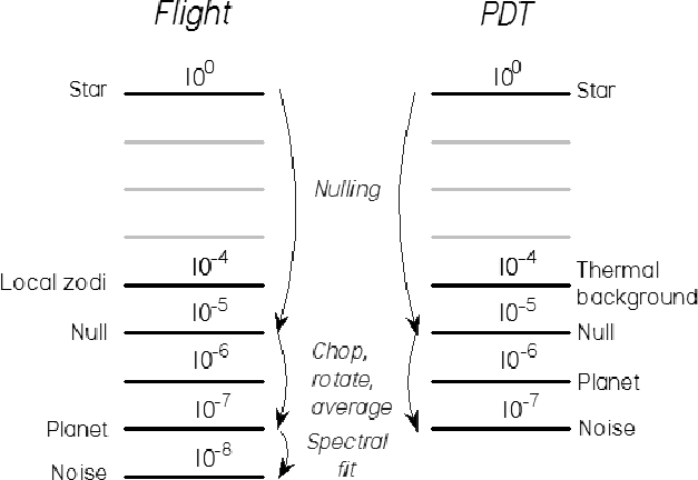
$\begin{figure} \par\resizebox{9cm}{!}{\includegraphics{14942fig1.eps}} \end{figure}$	Figure 1: Exoplanet detection process using a nulling interferometer.
Open with DEXTER

Figure 1 (left) illustrates the exoplanet detection technique envisaged for TPF-I.

1.: the star's apparent intensity is reduced relative to the planet by a factor of 100 000. This is done by interferometric nulling;
2.: the interferometer array is rotated around the line of sight to the star to search the region around the star for a characteristic planet signature;
3.: the planet signal is modulated against the bright radiation background. This is done using phase chopping. The combination of rotation, phase chopping and averaging over time reduces the noise level by a factor of one hundred, to 10^-7 of the stellar intensity;
4.: The technique of spectral fitting uses correlations between null fluctuations across the spectral band to reduce the instability noise. This yields a further factor of ten in reduction of the noise level.

The successful combination of these four techniques will yield the performance needed to detect an exo-earth. In this work, as shown on the right of Fig. 1, the objective was to demonstrate the first three parts of this process; the stable nulling, the array (or planet) rotation and the phase chopping. The fourth part, spectral fitting, requires a broadband source (the testbed has only a monochromatic source for the star) and a spectrometer and so is not addressed here.

This paper covers a description of the PDT, an outline of its capabilities, the objectives of the test and the demonstration criteria. There follows a description of the reduction and analysis of the collected data. Finally the results and conclusions are given.

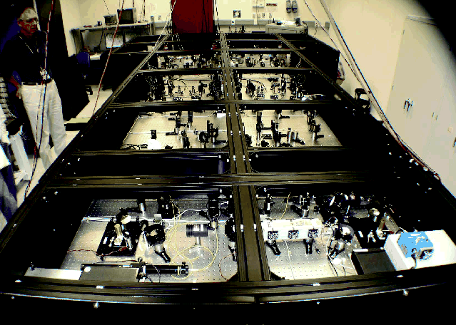
$\begin{figure} \par\resizebox{9cm}{!}{\includegraphics{14942fig2.eps}} \end{figure}$	Figure 2: The planet detection testbed, PDT, seen from the source end.
Open with DEXTER

2 The planet detection testbed

2.1 Principle and objectives of the testbed

The planet detection testbed, pictured in Fig. 2, was developed to demonstrate the feasibility of four-beam nulling, achievement of the required null stability and the capability of detecting faint planets using approaches similar to the ones contemplated for a flight mission such as TPF-I or Darwin/Emma (Cockell et al. 2009). The most promising architectures for a flight mission employing synthesis imaging techniques (the X-array, Lay et al. 2007 and the Linear Dual-Chopped Bracewell, Lane et al. 2006) are four-beam nulling interferometers that use interferometric chopping to detect planets in the presence of a strong mid-infrared background. Some other effects of this background on interferometer performance have been discussed by Defrère et al. (2010).

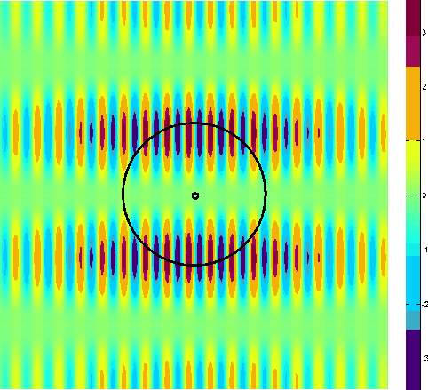
The flight mission will use the phase chopping (Woolf & Angel 1997) technique to modulate a sensitivity/fringe pattern around the star. This modulation technique is in many ways similar to the use of a chopper wheel that allows the detection of infrared sources against a thermal background and/or drifting detector offsets. In this case the thermal background on the sky includes the local and exozodiacal light. To achieve this modulation the interferometer employs two nullers each phased to null out the starlight and a second beam combiner, known as the cross-combiner, combines the output from the nullers and phases it to form the moving sensitivity pattern. The effect is to create a fixed dark null fringe over the star and also, moving constructive fringes which allow light from other parts of the field of view to enter the detector. The constructive fringes move stepwise, alternately to each side of the star and thus may move on and off the planet. If there are other planets in the field of view, their signals will also contribute depending on their locations and by rotating the fringe system around the star the whole planetary system can be observed. Signal processing is then used to determine the location of the planets orbiting the star. For a TPF-Emma X-array with 6:1 aspect ratio, the aperture layout and chopping action results in the on-sky modulation pattern shown in Fig. 3. In the figure, the modulation ranges from -1 to 1 (dark blue through green to dark red). The star is situated at the center. As the formation of telescopes rotates, the light from a planet will be modulated in a way characteristic of its angular distance from the star.

$\begin{figure} \par\resizebox{9cm}{!}{\includegraphics{14942fig3.eps}} \par\end{figure}$

Figure 3:

On-sky monochromatic modulation pattern for the TPF-Emma X-array. The small circle denotes the position of the star and the large circle the path traced by a planet through the fringe system as the formation rotates. The plot has been apodized to illustrate the effect of the field of view of a single mode fiber in the detection system: in reality the field of view would be a minimum of 20 fringes wide in the horizontal direction.

Open with DEXTER

The primary objective of the Planet Detection Testbed is to simulate this observing scenario and demonstrate the instrument stability needed to make this process work. The testbed is intended to demonstrate control of the nullers and the cross-combiner at levels close to those needed for flight, in the presence of ambient laboratory noise and optical disturbances. (Under Appendix A there is a discussion on the differences between the testbed and flight operations and conditions.) On the PDT a realistic planet signal can be created by controlling the optical path relationships between four planet source beams, simulating the phase changes caused by rotation of the telescope array around the line of sight to the star. Moreover, as a four-beam combiner, the testbed produces instability noise (Lay 2004); the testbed has systems and control loops analogous to those needed for flight in order to control the instability noise and maintain deep nulls.

At the output, the detected signal is the difference in the measured photon flux between the two chop states and this signal has both stochastic and systematic noise components. The time-varying part of the systematic component comprises the instability noise, which is expected to have a 1/ $\textit{f}$ spectral dependence. Such 1/ $\textit{f}$ disturbance spectra are fairly weakly suppressed by increasing experiment duration while, for white noise spectra, suppression improves with the square root of the duration. Typical values of instability noise suppression predicted for our test protocol (rotation, chopping and averaging) were between about 25 and 50, compared with white noise suppression of between a few hundred and a few thousand for likely experiment durations. The target suppression of the instability noise of 100, being between these two limits, would be achieved by a reduction of a part of the natural 1/ $\textit{f}$ disturbance spectrum by the testbed control systems. (The instability noise can be further reduced using expected correlations across the broadband light spectrum: this is the basis of the spectral fitting technique, but that was not employed here.)

$\begin{figure} \par\includegraphics[width=9cm,clip]{14942fig4.eps} \end{figure}$

Figure 4:

Schematic layout of testbed beam train. Star and planet light enters from the lower left through individual synchronized choppers. Each beam is then split twice to create four beams of starlight and four of planet light. These eight beams are then combined to make four beams, one for each TPF telescope. These four beams are then passed in pairs through two nullers and thence to a cross-combiner. One output of the cross-combiner goes to a detector. Planet phases are controlled by five moving optics; four mirrors and the first planet beam splitter. The phases at the nullers are controlled similarly using a set of mirrors. Finally, the cross-combiner imposes a $\pm$ $\lambda$ /4 phase chop.

Open with DEXTER

2.2 General description of the testbed

The PDT is built on a large T-shaped optical table comprised of a $12\times 6$ ft table bolted to a $10\times 5$ ft table. It is mounted on a pad, separated from the main floor of the building, on eight vibration absorbing air legs. The table is completely enclosed by a cover consisting of a frame covered with removable aluminum honeycomb panels, which provides partial isolation from room temperature changes and air conditioning turbulence. The testbed has the following main components: a star source and a planet source, a pair of nullers to null out the starlight and a cross-combiner to allow modulation of the detected planet signal. To provide the necessary stability, the testbed has pointing and shear control systems, laser metrology systems and fringe trackers to maintain the phase on the star. Reviews of the development of the testbed and some of the systems may be found in Martin et al. (2005), Martin (2006) and Booth et al. (2008).

The testbed produces four mid-infrared beams of light from the star and another four from the planet, then combines star and planet beams in pairs to produce four star+planet beams as if detected by the four telescopes. These beams are then nulled and cross-combined. Figure 4 shows the key parts of the optical layout. The beam combination process reproduces the operation of the flight beam combiner (Martin 2005). Using the delay lines, a $\pi$ phase shift is introduced into one of each beam pair by a combination of optical path differences in glass and air, producing a null at one output of each of the nulling beam combiners. The input star and planet beams are passed between chopper blades in a standard method for detecting faint infrared signals in the presence of a stronger background. These choppers are synchronized so that the star and planet are chopped (shuttered off and on) simultaneously. The precise detection process is discussed in detail below.

As shown in Fig. 5, the outputs of a CO₂ laser and a thermal source (a hot filament) are combined to form the star. The laser light provides 10.6 $\mu$ m wavelength radiation which is to be nulled and the thermal source provides broad band radiation, of which, radiation between 2.2 and 2.53 $\mu$ m is used for fringe tracking on the star. The starlight is passed through a chopper and pinhole and then split into two beams. These beams are split again forming four beams (the functional parts of one beam are labeled in the figure and are reproduced in each beam) and, after this second splitting stage, combined with four beams from a second thermal source. This second source, limited to a band of radiation 1 $\mu$ m wide and centered at 10.5 $\mu$ m, forms the artificial planet.

The overall optical throughput of the testbed varies with wavelength but near 10 $\mu$ m, the source area throughput is $\approx$ 56% (excluding nominal losses at beam splitters). Most loss is at the input pinhole. The beam-combiner area throughput is $\approx$ 24% (excluding beam splitters). At the detector, an 8 $\mu$ m diameter pinhole is used to provide spatial filtering. The loss at this component is approximately 50%. In flight, more efficient single mode fiber spatial filters will be used (Ksendzov et al. 2008).

2.3 Control systems

The four starlight beams are controlled by near-identical systems. Each beam has a fast and a slow optical delay line enabling both rapid, fine control of optical path length and slower, coarse control. The slow control can, for example, compensate for slow drifting of the overall optical path caused by thermal changes in the laboratory. The fast delay lines can compensate for higher frequency changes in optical path length caused, for example, by vibrations. The control signals for the delay lines are derived from the outputs of two sets of sensors. One, the laser metrology system, provides three measurements of optical path along sections of each beam train, so there is a total of 12 metrology signals. This measurement system provides a fast response to vibrations and has a small drift at longer (tens of seconds) timescales. The second path length sensor is the fringe tracker which has a slow response ( $\approx$ one second) but can provide one nanometer accuracy or better. The fringe tracking signal is available when two starlight beams combine on a nulling beam splitter. There is a total of three fringe trackers, one for each nuller and one for the cross-combiner.

Each beam has two piezoelectrically controlled tip/tilt mirrors. The first mirror (in combination with the second) allows for adjustment of the shear of the starlight within each beam train and the second mirror is used to adjust the pointing. The control voltages exerted on these two mirrors enable the intensity of the light striking the detector to be held constant to the 0.2% level, an important requirement for stable nulling. The control signals for these mirrors come from a pair of quad cell sensors mounted near the nulling beam splitters. The sensors derive their signals from a diode laser beam injected into the beam train before the first beam splitter. This laser beam follows the path of the star's radiation and thus provides a reference to the starlight pointing and shear within the testbed. One sensor measures shear to $\approx$ 10 $\mu$ m sensitivity and the other measures pointing to $\approx$ 1 $\mu$ radian sensitivity.

Each beam has a phase plate (Morgan et al. 2000) which enables correction of the small (<4 $\mu$ m) thickness differences between the beam splitters. By adjusting the phase plates to certain thickness differences, phase differences between the 10 $\mu$ m radiation and the fringe tracking radiation near 2.3 $\mu$ m can be adjusted so that the fringe trackers have maximum sensitivity when the 10 $\mu$ m starlight is being nulled.

Referring again to Fig. 4, at the two nulling beam splitters, each pair of starlight beams is combined and then at the cross-combiner all four beams are combined. At that location a delay line called the chopping stage enables a phase difference to be produced between the outputs of the two nullers. This phase difference, which is introduced at a 2 s period, causes the planet signal to be modulated. The chopping stage has been designed to move $\approx$ 6 $\mu$ m with extremely low induced beam tilt, for stable performance.

$\begin{figure} \par\includegraphics[width=9cm,clip]{14942fig5.eps} \end{figure}$

Figure 5:

Schematic layout of testbed optical systems. Only one beam path, the lowest one, is shown in its entirety since the three other beam paths have identical systems. The lines represent the light paths which travel generally from left to right. Top half of figure, the source area, the light from each source is shown being split from a single beam into four beams; A, A', A'': respectively, thermal source for planet, and laser and thermal sources for star; B, B': synchronized chopper blades; C: planet source metrology retro-reflector; D: first beam splitter in planet path, with delay line; E: first beam splitter in star path; F, F': second beam splitters; G: planet phasing mirrors; H: star-planet beam combiners (eight beams merge into four star and planet beams); J: pointing and shearing alignment laser entry point; K: planet metrology entry point. Bottom half of figure, the beam-combiner area, four beams merge into a single beam; L: intensity adjuster; M: beam combiner metrology entry point; N: pointing and shearing adjuster mirrors; Q, R: pointing and shearing sensing; P: fast and slow delay lines; S: nulling beam combiners; T: two nuller fringe tracker outputs; U: chopping cross-combiner (one beam emerges for detection); V: two cross-combiner fringe tracker outputs; W: beam combiner metrology retro-reflector; Y: spatial filter; Z: nulling detector.

Open with DEXTER

$\begin{figure} \par\includegraphics[width=9cm]{14942fig6.eps} \end{figure}$	Figure 6: Calculation of the planet phase for each beam input. The circles T represent the telescope formation rotating around the center at radii L. The phase of the planet light is measured along the bold line which passes through the star and planet.
Open with DEXTER

2.4 Production of the planet signal

The planet detection method involves simulation of a rotation (or rotations) of the telescope array while nulling the star. By adjusting the relative phases of the planet beams, the apparent wavefront from the planet can be tilted so that the incoming planet light effectively makes a slight angle to the star light. 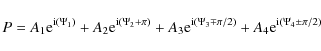By varying that tilt in a controlled sinusoidal fashion the testbed simulates the telescope array rotation around the line of sight to the star. The phase $\Psi_{i}$ for the ith telescope is given by:

$\begin{displaymath}\Psi_{i}= \frac{2 \pi L_{i} \Omega} {\lambda}\cos\left(2 \pi \omega t + \theta_{i}\right) \end{displaymath}$

(1)

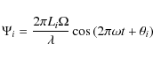
where L_i is the distance of the ith telescope from the formation center, $\lambda$ is the infrared wavelength, $\Omega$ is the angular offset of the planet from the star, 2 $\pi\omega\textit{t}$ is the rotation angle of the array and $\theta_i$ is the angle made by the ith telescope to a line bisecting the array; see Fig. 6. For the testbed, we chose values of displacement on the planet phase control stages to give realistic values of L $\Omega$ . By choosing different values of L_i and $\theta_i$ we could set up X-array formations or linear formations. The corresponding amplitude for the planet signal is simply given by:

$\begin{displaymath}P = A_{1}{\rm e}^{{\rm i}\left(\Psi_{1}\right)} + A_{2}{\rm e... ...right)} + A_{4}{\rm e}^{{\rm i}\left(\Psi_{4}\pm\pi/2\right)} \end{displaymath}$

(2)

where the A_i are the input beam amplitudes and both chop states are represented by $\pm$ $\pi$ /2. As the formation rotates, the phases of the planet beams evolve sinusoidally, with a different initial phase for each input. To generate these phases the testbed employs 4 mirrors and a beam splitter which follow sinusoidal piston paths with different phases controlled by the testbed metrology system. For an X-array formation, the distances L_i are all equal and $\theta_1=-\theta_2=\theta_3-\pi=\pi-\theta_4$ . So for a pair of planet beams arriving at apertures 1 and 2, a nulling pair, the differential phase is given by:

$\begin{displaymath}\Psi_{1}-\Psi_{2}=\frac{-4 \pi L \Omega }{\lambda}\sin\left(2 \pi \omega t\right) \sin\left(\theta\right) \end{displaymath}$

(3)

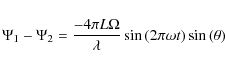
On the long baseline between apertures 1 and 4 we obtain similarly:

$\begin{displaymath}\Psi_{1}-\Psi_{4}=\frac{-4 \pi L \Omega }{\lambda}\cos\left(2 \pi \omega t\right) \cos\left(\theta\right) \end{displaymath}$

(4)

The scaling factor tan( $\theta$ ) between 3 and 4 is equal to the aspect ratio of the X-array formation. By measuring the differential phases $\Psi_{1}-\Psi_{2}$ , $\Psi_{3}-\Psi_{4}$ and $\Psi_{1}-\Psi_{4}$ using the metrology system, correct differential phases can be calculated for the input planet beams to mimic a planet signal at any chosen angular separation $\Omega$ . In the testbed implementation, two of the mirrors execute open-loop, approximately sinusoidal motion, while the two other mirrors and the beam splitter execute motions under closed loop control. This results in the exact desired effect within the resolution and stability of the metrology system. The apparent angular distance of the planet from the star is set by the amplitude of the control signals applied to the planet mirrors. Across the short array baseline (between a pair of beams which would be nulled) the planet mirrors were controlled to produce a sinusoidal optical path difference (OPD) variation in air of amplitude 6.2 $\mu$ m. Across the long baseline, the motion created a co-sinusoidal OPD variation of 37.2 $\mu$ m amplitude, thus emulating an X-array formation with a 6:1 aspect ratio.

2.5 Detection and measurement of the planet signal

Characteristic planet signals would be obtained from the beam combiner depending on the spacecraft formation geometry and the distance of the planet from the star. As can be inferred from Fig. 3, for different planet angular separations from the star, different paths will be traced through the interferometer's transmission map. Then, for any planet angular separation, a template can be produced that corresponds to the transmission function for a single formation rotation. The planet signal, which will contain substantial instability noise, will be tested by cross-correlating the measured signal for one rotation with a series of planet signal templates.

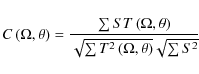
The two principal analyses are: the detection of a planet signal (for planet-only and star-and-planet), and the measurement of the noise at a given planet angular separation (star-only). We create the templates, as discussed by Mennesson & Mariotti (1997), for a 6:1 X-array formation of telescope apertures. For a recorded testbed signal S, truncated to an integer number of array rotations, and templates T( $\Omega$ , $\theta$ ) where $\Omega$ is the angular separation from the star and $\theta$ is the rotation angle, we calculate the cross-correlation:

$\begin{displaymath}C \left(\Omega,\theta \right)=\frac{\sum S T\left(\Omega,\the... ...\sqrt{\sum T^2 \left(\Omega,\theta \right)} \sqrt{ \sum S^2 }} \end{displaymath}$

(5)

for all desired template signals, using values of $\Omega$ starting near the star and extending outwards, and testing at all rotation angles $\theta$ (0 to 2 $\pi$ ).

Figure 7A shows the signal template for a planet at an angular separation of $0.635 \times 10^{-6}$ radian (130 mas) from the star. The test process, applied to that template signal for example, yields a two-dimensional map of the correlation in space as shown in Fig. 7B. Since the template signals for planets located throughout the observed region of space can correlate to some degree with the actual planet signal, a kind of bulls-eye pattern, with anti-symmetry, is observed, the planet being located at the positive peak of the correlation.

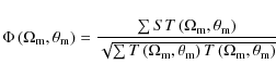
The detected planet will be assumed to be at the location ( $\Omega _{\rm m}$ , $\theta _{\rm m}$ ) where the cross-correlation is a maximum. Then the following equation is used to obtain an absolute measure of the signal amplitude at that location:

$\begin{displaymath}\Phi \left(\Omega_{\rm m},\theta_{\rm m} \right)=\frac{\sum S... ...{\rm m} \right) T\left(\Omega_{\rm m},\theta_{\rm m} \right)}} \end{displaymath}$

(6)

The true rms of the detected planet signal ( $\sigma _{\rm P}$ ) at this location (rather than the rms of the signal trace which contains some noise), is the rms of a template signal T at ( $\Omega _{\rm m}$ , $\theta$ ), with amplitude $\Phi$ . Thus from the similar Eqs. (5) and (6), five quantities, $\Omega _{\rm m}$ , $\theta _{\rm m}$ , $\Phi$ , C and the detected signal rms are obtained.

If no planet signal is present but S contains instability noise, the signal at any location ( $\Omega$ , $\theta$ ) is a measure of part of the noise. So, to obtain the signal to noise ratio for the planet in the star-and-planet trace, we compare $\sigma _{\rm P}$ to the rms of the star-only signal at the planet angular separation $\Omega _{\rm m}$ . This is done by applying the template T to the star-only signal at the measured angular separation $\Omega _{\rm m}$ of the planet and calculating $\Phi$ for all angles $\theta$ . The rms of $\Phi$ ( $\Omega _{\rm m}$ ,0 to 2 $\pi$ ) is the noise rms ( $\sigma _{\rm n}$ ).

$\begin{figure} \par\includegraphics[width=9cm]{14942fig7.eps} \end{figure}$

Figure 7:

A: the planet signal template for a planet at an angular separation of $0.635 \times 10^{-6}$ radian (130 mas) from the star, utilizing the formation parameters given in the results section. B: the corresponding correlation map on the sky when this template is tested using all the templates for planets at angular separations from $0.2 \times 10^{-7}$ radian (4 mas) to $1.75 \times 10^{-6}$ radian (360 mas). The planet's location is at the peak of the correlation at ( $6.35 \times 10^{-7}$ , 0) radian. The vertical scale of the correlation ranges from -1 (blue) to +1 (red).

Open with DEXTER

The star-only signal is used for this measurement because if the signal contained a planet, the noise level will be only an estimate. It would be found by subtracting the fitted planet signal from the trace and testing again. Since the fitted planet signal will contain some of the noise, the result will be the noise minus some fit error and will be an underestimate of the background noise.

Table 1: Summary of data sets taken in June and July 2009.

Table 2: Summary of data sets presented here.

3 Demonstration criteria

The goals of the demonstration were to meet the following performance criteria:

1.: residual starlight suppression, after nulling, resulting from phase chopping, averaging and rotation, of at least one hundred;
2.: detection of a planet, at a signal to noise ratio of at least ten, at a contrast of at most 10^-6 relative to the star;
3.: stable performance for at least 10 000 s (with periodic resetting allowed);
4.: repeatability of the performance.

Criteria 1 and 2 are discussed in more detail in Appendix B, together with some additional definitions and context for the ladder diagram (Fig. 1). The starlight suppression level is at the flight requirement and would allow Earth-like planet signal extraction when the spectral fitting method is also employed. The time-series duration of at least 10 000 s demonstrates long-term stability of the system, which approaches flight-level requirements of (typically) 50 000 s.

The following test procedures were designed to show: suppression of the starlight by a factor of one hundred below the null (planet source off), thus satisfying criterion 1, generation and detection of a planet signal ten times fainter than the null, thus satisfying criterion 2, sufficient test run-times to satisfy criterion 3, and repeatability of the performance to satisfy criterion 4.

Star-only test. The testbed was set up with all normal systems running except that the planet source was off. Measurements were made of the nulling detector output, which consists principally of the star laser light leakage. Data processing established the starlight suppression ratio after chopping and averaging. The test ran for at least 10 000 s.
Planet-only test. A measurement of the absolute planet signal magnitude was obtained by running a test with all normal systems running except that the star's laser source was off. This yielded a planet signal free of instability noise but with any other noise still present. The test verified that the planet path lengths are being correctly controlled and also yielded a measurement of the planet signal intensity so that the star to planet intensity ratio could be calculated. The test ran for at least 2000 s (or one rotation of the planet).
Star-and-planet test. A detection of the planet signal was made by running a test with similar conditions to the first two tests but with both planet and star sources on. The planet signal was detected in the data and could be compared with the planet-only signal. The suppression ratio was be assumed to be that found under item 1. The test ran for at least 10 000 s.
Repeatability test. These tests were run a total of three times on different days. Each test was separated by at least 48 hours from the previous test in order to verify the repeatability of performance.

4 Description and analysis of the collected data

4.1 Overview of the results

Several sets of data (shown in Table 1) were acquired that satisfied the technical criteria numbered 1, 2 and 3 (above). Because they were not all spaced more than 48 h apart (only nearly so), thus failing on criterion 4, we have chosen to fully review only a subset of these data sets in this paper. These data sets collectively meet all the criteria. Other combinations of data sets could have been chosen that would also satisfy all the criteria. Table 1 briefly summarizes all the data sets taken between mid-June and the end of July 2009. Four data sets were rejected because, in those cases, the planet signal amplitude did not fit the ${\it SNR} = 10$ criterion. However, since criterion 1 (residual starlight suppression) was satisfied in all but one case, there are planet amplitudes even in the rejected cases that would have met criterion 2, had we set up the testbed systems appropriately. Indeed, one of the more difficult parts of the test setup was to reliably place the planet intensity into the central range between the null and the noise. This was because 1: the star laser's intensity was different on different days; 2: adjustment of the planet signal was difficult because it was very weak and therefore difficult to measure accurately in a direct way and 3: the noise floor also varied. The noise floor is influenced by the disturbance environment in the building in which the laboratory is contained and seemed to vary daily. However, the overall starlight suppression was in all cases 25 million to one, or better. The suppression of the starlight beyond the null, obtained by chopping, averaging and rotation, ranged between 89 and 326, meeting or exceeding our minimum goal of 100 in all but one case.

Table 2 summarizes the main results for the selected data sets against the demonstration criteria. For the data sets of 6-18, 7-10 and 7-23 all the demonstration criteria were satisfied. In each case the residual starlight suppression from phase chopping, averaging and rotation was >100, thus satisfying criterion 1. The planet-to-star contrast was less than 10^-6 with a planet ${\it SNR}>10$ , thus satisfying criterion 2. The tests each ran for a duration >10 000 s, thus satisfying criterion 3. Criteria 1 to 3 were satisfied simultaneously on three separate occasions with at least 48 h between each demonstration, thus satisfying criterion 4.

Figure 8 compares the principal results against the test criteria in graphical form. The plot is similar in form to the ladder diagram, with the star at unity and the corresponding levels for the results visualized as bars. In summary, all of the success criteria for the demonstration were met or exceeded. Details of the data processing and resultant data plots are provided in the following subsections.

$\begin{figure} \par\includegraphics[width=9cm]{14942fig8.eps} \end{figure}$	Figure 8: The test performance data summarized in the ladder diagram form. The principal measured performance levels for the three data sets are compared with the demonstration goals. The null depth, the planet signal $\Phi$ ( $\Omega _{\rm m}$ , $\theta _{\rm m}$ ), the planet rms $\sigma _{\rm P}$ and the rms noise $\sigma _{\rm n}$ are shown compared with the normalized starlight (unity).
Open with DEXTER

4.2 Data reduction procedure

Three main data files were acquired for each run together with a number of ancillary supporting files. These files are pre-processed to obtain a subset of the data, and then this reduced data set is subjected to a series of processing steps. The data, sampled at 5 kHz, was sub-sampled and logged to disc at 50 Hz (in most cases) producing data sets of more than 500 000 samples per record. Planet-only files were shorter since only one rotation was required, resulting in initial record sizes of more than 100 000 samples.

$\begin{figure} \par\includegraphics[width=9cm]{14942fig9.eps} \par\end{figure}$

Figure 9:

The signal processing steps shown in order for the star-only data of the 6-18 data set: A, normalized data from nulling detector, truncated to 600 000 samples, representing a 12 000 s run time. B, the data processed in synchrony with the cross-combiner chop at a 2 s period. Reset periods have been removed and the record is now 10 000 s long. C, the chopped data cyclically averaged over the five rotations; now 2000 s long. D, data (C), high-pass filtered to remove only the dc level and the first harmonic of the rotation and the reset periods.

Open with DEXTER

Figure 9 shows full length time series records of the nulling detector output for the star-only run of the 6-18 data set. The vertical axes show contrast normalized by the total starlight (for clarity the axis of Fig. 9A is limited to a reduced range), the horizontal axes show sample number. The graph 9A exhibits two distinct characters. One, what appear to be periodic full range bursts occur during the reset periods. Two, the intervals between show the detector output sampled at 50 Hz. The two-beam null depth on the nullers can be estimated from this graph: it is approximately twice the mean of the trace, as noted in Appendix B. (For the purpose of establishing the levels for the data reduction, we made separate measurements of the individual nuller performances.) The data is next reduced by selecting the chopped data and eliminating the reset intervals, producing a record more than 5000 samples long, which is sampled at 0.5 Hz, to produce Fig. 9B.

The star-and-planet and the star-only data sets were sufficiently long to contain five rotations of the array (whether or not the planet was active). To average either of these two kinds of data, sections of length 2000 s (one rotation period) were overlayed and summed point by point, then divided by five, resulting in a record exactly 1000 samples long, sampled at 0.5 Hz, as shown in Fig. 9C. In the case of a planet-only record, this step was skipped and the data was simply truncated to a length of 1000 samples. To remove any dc offset and low frequency ripple, the record was then filtered by taking the Fourier transform, zeroing the first three terms and transforming back, resulting in the trace shown in Fig. 9D. This transformation results in elimination of the dc offset, the fundamental of the rotation period and the fundamental of the reset period. Figure 10 shows a similar data set for the star-and-planet data from 6-18. Thus prepared, the data was ready for testing for the presence of a planet signal.

$\begin{figure} \par\includegraphics[width=9cm,clip]{14942fig10.eps} \end{figure}$	Figure 10: The same signal processing steps shown in order for the star and planet signal of 6-18: A, normalized data from nulling detector. B, the data processed in synchrony with the cross-combiner chop. The planet signal is already apparent. C, the chopped data cyclically averaged over the five rotations. D, data (C), high-pass filtered, showing a clear but noisy planet signal.
Open with DEXTER

4.3 Planet template signal modification

Table 3: Summary of data sets presented here.

Because of a small uncommon path error arising between the star and planet (see Appendix C for details), the template signals must be modified to match the actual generated planet signal for each data set. This is done by performing the correlation test on the star-and-planet or planet-only data to determine approximate values of $\Omega _{\rm m}$ , $\theta _{\rm m}$ and $\Phi$ and then using the Matlab $^{\textregistered{}}$ function fminsearch to find an asymmetry value $\alpha$ . Once $\alpha$ is determined, the template signals used in all subsequent data processing include this asymmetry factor. When measuring the rms noise level we chose the asymmetry value measured for the star and planet, rather than trying to fit an asymmetry value to the data. Tests using asymmetry values over the range 0 to 2 $\pi$ showed that the choice of asymmetry value for this measurement had a negligible effect (less than 1%) on the measured rms noise level.

5 Results

Table 3 summarizes the data for the three datasets. The stellar intensity (row A) is normalized to unity and all the other data is normalized by the same factor. The upper part of the table shows the measured normalized quantities and the lower half shows the quantities of interest for the demonstration. The two beam null depth (row B), the planet signal (row C), and the noise rms (row F) are defined in B.2. The measured planet signals (rows D and E) are the results of the data testing algorithms, i.e. the output of the detection process applied to the testbed detector output. The star-to-null quantity, row G, is row A divided by row B. The star to planet quantity, row H, is row A divided by row C. The null to planet quantity, row I, is row B divided by row C. The planet to noise quantity, row J, is row E and the rightmost of the two columns, divided by row F. It compares the detected planet rms obtained from the star-and-planet run with the detected noise rms obtained from the star-only run. The suppression below the null, row K, is row B divided by 2, divided by row F.

Two sets of planet data are presented for each data set corresponding to the planet amplitudes measured in the two runs, planet-only and star-and-planet. In the lower part of the rightmost column, the target values matching the demonstration criteria are shown. Each data set meets all these criteria. In the lower-most row, the suppression of the starlight below the null is expressed as the two beam null depth divided by the rms noise. In Tables 1 and 2, this value was also more conservatively expressed in an alternative form as the product of the planet to null ratio and the rms planet to rms noise ratio (row I times row J).

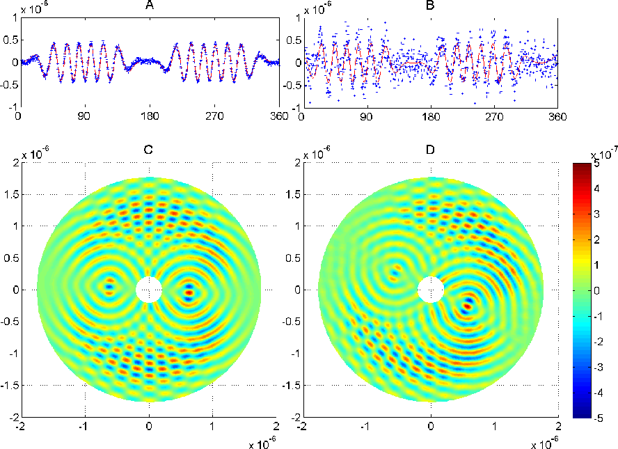
$\begin{figure} \par\resizebox{15cm}{!}{\includegraphics{14942fig11.eps}} \end{figure}$	Figure 11: Summary plots normalized by the stellar intensity. A: planet-only signal data and fit. B: star-and-planet signal data and fit. C: planet-only signal, cross-correlation map of $\Phi$ in space. D: star-and-planet signal, cross-correlation map. E: star-only cross-correlation map and for comparison, F: cross-correlation map for D with the detected planet signal removed.
Open with DEXTER

Figure 11 shows a summary of the data for the 6-18 data set. Data is normalized by the stellar intensity. Figure 11A shows the signal for the planet-only run, the blue dots, and the red trace shows the planet signal fit. Figure 11B similarly shows the signal and fitted planet signal for the star-and-planet run. Figures 11C and D show the corresponding cross-correlation maps of $\Phi$ in space. In both cases the peak indicating the location of the planet is to the right of center and the ``anti-peak'' is to the left: in the star-and-planet case the plot is rotated because the planet motion was started approximately 4 min before the data acquisition commenced. The central white area is an area not scanned for the planet.

The maps shown do not extend out to the full area over which the planet could be detected in the conceptual full TPF-Emma mission; for clarity only the central portion is shown. In reality the map would be several times wider, depending on the reciprocal of the telescope primary mirror diameter. The angular units assume an array nulling baseline, corresponding to the distance between apertures 1 and 2, of 10 m, suitable for detecting an exoplanet at 1 AU from its parent star at a distance of 10 pc. (The choice is fairly arbitrary; in the TPF-Interferometer design, we can utilize short baselines up to $\approx$ 70 m to obtain higher angular resolution). To convert these units to an OPD (optical path difference) between apertures 1 and 2, multiply by 10 million to obtain OPD in micrometers. Thus we see in Table 4 (discussed further below), that the measured planet orbital angular separations correspond reasonably closely with the set-up OPD of 6.2 $\mu$ m. Figure 11E shows the star-only cross-correlation map and Fig. 11F shows the star-and-planet cross-correlation map with the detected planet signal removed; some noise peaks remain but with little structure evident that would be associated with a planet signal.

$\begin{figure} \par\resizebox{16.5cm}{!}{\includegraphics{14942fig12.eps}} \end{figure}$	Figure 12: Summary plots for data of 7-10.
Open with DEXTER

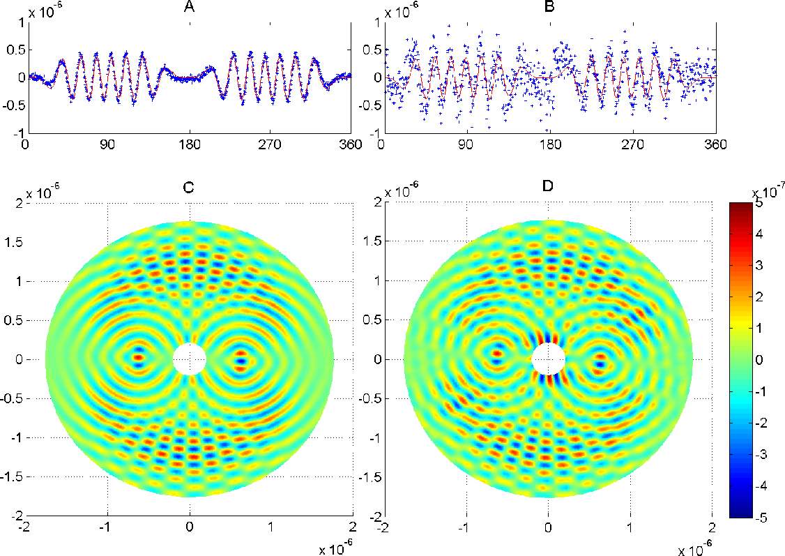
$\begin{figure} \par\resizebox{17cm}{!}{\includegraphics{14942fig13.eps}} \end{figure}$	Figure 13: Summary plots for data of 7-23.
Open with DEXTER

Figures 12 and 13 show similar graphs for the other two data sets. (The plots of star-only cross-correlation and of the residual after the removal of the planet signal are not included since they are very similar in appearance to those in Fig. 11.) In the data set of 7-23, because of a reconfiguration of the planet metrology optics, the array rotation was retrograde with respect to the other data sets and so the planet appeared approximately $\pi$ radian away from its former position, to the left of center instead of to the right.

Table 4 shows the supplementary data produced from the demonstration runs. As expected, planet-only data had a high correlation with the model, using the fitted asymmetry values. For the star-and-planet data, the correlation coefficients were more modest but the planet orbital radii agreed very closely with the planet-only data. The planet phases are expected to differ because of execution timing differences between runs but agree well with the corresponding metrology data estimates. For example, Fig. 14 shows a planet signal constructed from the metrology data assuming four equal amplitude beam inputs (blue dots), and its fitted signal (red line). The data set of 6-18, planet-only is shown. The correlation coefficients obtained for these fits were between 0.98 and 1.00. These metrology estimates were used to verify the detected phase angles shown in Table 4. The slight differences between the fit and the modeled signal may arise from the simple modeling of the planet spectrum as a ``top-hat'', flat between 10 and 11 $\mu$ m.

Taking the data sets as a whole, the agreement between the angular separation data measured from the star-and-planet signals and the planet-only signals is good; the rms difference is 0.7%. The agreement between the angular separation data measured for both the star-and-planet signals and the planet-only signals compared with their respective simulated signals derived from the metrology is similar; the rms difference is also 0.7%. The fit resolution for the angular separation is $0.01 \times10^{-7}$ radian (0.2 mas). Planet signal phases were in good agreement with the metrology-derived phases. The fit resolution is 0.01 radian in phase angle and the results all agree to within 0.02 radian. The rms asymmetry value $\alpha$ is 0.35 radian (20 $^{\circ}$ ) corresponding to about 600 nm of uncommon path error which could result from a typical mean temperature change of the testbed face-sheet of 60 mK between set-up and test execution.

Table 4: Supplementary data reduction values.

6 Conclusions

The data show that the combination of starlight nulling, phase chopping, array rotation, averaging and fitting to predicted planet signals (matched filtering) yields strong starlight and instability noise suppression. In the three tests, the resulting suppression of the starlight at the planet angular separation was by a factor of at least 67 million. Planet signals were obtained from the testbed having a good match to theoretical signals and only a single parameter was modified to account for a small uncommon path error. Analysis of the angular separation of the planet signals detected by nulling showed an excellent match to the actual metrology-controlled mirror displacements and the phasing of the detected signals was similarly well-matched by metrology signal analysis. The tests were conducted with an eye towards space operations:

There was no operator intervention during the data-taking.
The initial null depth was limited to the 10^-5 level, similar to the level expected to be used in space.
The testbed was allowed to drift from the initial alignment and co-phasing and was reset at fairly sparse intervals.

The testbed demonstrated good stability despite its sensitivity to small environmental changes. In space, we would expect a more benign environment, but we would also run for longer periods ( $\approx$ 50 000 s typically). The tests were very repeatable and were successfully executed at the required performance level several times. The main difficulty experienced was with the narrow intensity slot in which the planet had to be placed; given numerous disturbing factors, this led to the rejection of some otherwise good data sets. All the criteria of the demonstration were met and we therefore conclude that the goals of the demonstration were accomplished.

Under the technology program at the Jet Propulsion Laboratory for the development of infrared nulling for TPF-I, the principal optical tasks were divided into achromatic phase shifting architecture evaluations (Gappinger et al. 2009), adaptive nulling (Peters et al. 2008), single mode fiber development (Ksendzov et al. 2007,2008), and four-beam nulling. That work, which achieved the goals of adaptive nulling at the 10^-5 level over a 30% bandwidth and of higher mode suppression in single mode fibers of $1.5\times10^{4}$ , together with the starlight suppression of more than seven orders of magnitude and the planet detections reported here, met all the performance goals set for the technology program. (In addition, a formation flying testbed (Scharf et al. 2004,2010), met goals for spacecraft control that would be needed for the free-flying interferometer.) These performances, taken together, reach to within a factor of ten of the performance needed for flight.

$\begin{figure} \par\resizebox{8cm}{!}{\includegraphics{14942fig14.eps}} \end{figure}$	Figure 14: For the planet-only data of 6-18: the planet signal constructed from the planet beam train metrology data sampled at the chop frequency (blue dots) with the corresponding fitted planet signal measured from the mid-infrared detector.
Open with DEXTER

Additional work remains to be done and the current goal for the PDT is to expand the operation to broad band radiation, enabling testing of the final part of the starlight suppression plan as shown at the bottom left in Fig. 1. With the successful conclusion of that work, which is intended to close that factor of ten, the entire starlight suppression plan will have been demonstrated. Before moving to the initial stages of a flight project, further technology developments can be envisioned that would extend the work into the cryogenic area, with low radiation fluxes, increased optical bandwidth, and flight-like system architecture. While much is now being achieved in the exoplanet field by current telescope technologies, the eventual characterization of Earth-like exoplanets will depend on high performance observatories such as TPF-I and Darwin.

Acknowledgements

Kurt Liewer assisted with testbed development and operation. Frank Loya developed the software control system and several electronics systems. Oliver Lay assisted with development of the data analysis techniques and the traceability to flight. Hong Tang developed the testbed metrology system. Numerous others participated in testbed development over several years including Nasrat Raouf (optics), Piotr Szwaykowski (optical engineering), Randall Bartos (engineering), Boris Lurie (controls systems), Santos ``Felipe'' Fregoso (software), Francisco Aguayo (engineering), Martin Marcin (optical engineering), Ray Lam (software), Andrew Lowman (optical engineering), Steve Monacos (electronics engineering), Robert Peters (optical engineering) and Muthu Jeganathan (optical engineering). The authors are also grateful to Mike Devirian and to Peter Lawson for their unflagging support of the testbed. The work reported here was conducted at the Jet Propulsion Laboratory, California Institute of Technology, under contract with NASA. The mention of any commercial product herein does not constitute an endorsement. ©2010. All rights reserved.

Appendix A: Differences between flight and the laboratory demonstration

The testbed is fully representative of the flight architecture with beam shear and pointing control using a laser system, null stabilization using fringe tracking and with phase chopping at the beam combiner. However, there are several important differences between the lab demonstration and the baselined flight implementation: flux levels, representative control loops and calibration, timescales, polarization, ambient environmental conditions versus cryo-vacuum and detector types. Each is addressed briefly below.

Flux levels: Fig. 1 shows the key relative flux levels at a 10 $\mu$ m wavelength for (a) flight and (b) this test. Levels are normalized to the flux of the unsuppressed star. The exact ratios will depend on wavelength and the specific design of the flight system. The star is suppressed using nulling by a factor of 10⁵, bringing down the detected flux well below the level of the Local Zodi background. Chopping and averaging over the observation time reduces the level by a further factor of 10², down to the level of the planet at 10^-7. (This can also be viewed in the map domain; the planet signal appears in a single pixel, but the noise is scattered into many pixels. For a coronagraph Trauger & Traub 2007 this is the distinction between starlight suppression and contrast.) Spectral fitting is then used to achieve a further factor of 10 suppression of the noise relative to the planet, resulting in an SNR of 10. That technique exploits the spectral signature of the residual stellar leakage and it therefore requires a broadband star source. In this case, the star is simulated with laser light, so it is not possible to demonstrate spectral fitting. Therefore the levels shown for PDT in Fig. 1 are adopted for this test, with the planet intensity at 10-6 relative to the star. The absolute flux levels for PDT also differ by necessity from those in flight. In the flight scenario, the dominant source of background noise is emission from the Local Zodi ( $T\approx 300$ K, optical depth $\approx$ $4\times10^{-8}$ ). For the PDT the dominant source of background noise is emission from the ambient thermal background ( $T\approx 300$ K, optical depth $\approx$ 1), approximately $2\times10^{7}$ higher than the Local Zodi. All the photon flux levels for PDT are scaled up accordingly. There are two consequences: (1) the control loops and calibrations are operating in a significantly different flux regime. This is addressed below; (2) there will be negligible photon noise contributing to the null residual in the PDT experiment. The flight error budget has two main sources of noise: photon noise (straightforward to estimate given the flux level) and instability noise. The PDT experiment is addressing only the instability noise contribution. In a subsequent phase of the PDT we plan to demonstrate broadband nulling with spectral fitting, employing a bright, broadband arc source together with a low noise detector.
Representative control loops and calibration: maintaining a stable null over long periods in the presence of spacecraft motions requires a number of active control loops and calibrations, e.g. tip/tilt control, fast optical path difference control (metrology), slow optical path difference control (fringe tracking), equal intensity calibration, calibration of fringe tracking set points and adaptive nulling (a broadband phase and amplitude correction technique Peters et al. 2008). With the exception of adaptive nulling, all of these are represented in the PDT with an architecture that is scalable to flight. At this point however, we make no attempt to scale the PDT control loop performance to the flight conditions. There are 3 reasons for this: (1) the flux levels and detector performance differ by many orders of magnitude; (2) the flight disturbance environment is currently unknown but is likely very different from that seen in the lab; and (3) there are many layers of control and calibration with non-linear interdependencies that make it difficult to compare the various contributions between flight and testbed systems. While detailed model validation is a vital step in the future technology development for a flight mission, it is beyond the scope of the current tests. The controls architecture implemented in PDT is representative of flight, but the environmental differences mean that the quantitative performance characteristics are dissimilar.
Timescales: the baseline flight scenario calls for one or more rotations of the array per observation, with a typical rotation period of order 10 h. The current experiment is limited to timescales of less than $\approx$ 15 000 s by the ``hold time'' of the detector dewars. As for the discussion of control loops above, the PDT simulates the observation period over a period of several hours with a flight-like set of calibration steps, but the interval between recalibrations was not scaled in a quantitative way to flight timescales.
Polarization: in the flight system, the adaptive nuller component of the beam train will split the two linear polarization states and correct each independently for phase and amplitude deviations before recombining the light into a single beam. The PDT utilizes only one polarization of the laser light but uses no polarizing optical components; it would be expected to work equally well with either polarization state.
Cryo-vacuum: the flight system will operate in vacuum at low temperature ( $\approx$ 40 K), compared to the ambient air environment of the laboratory demonstration. The laboratory is a more challenging disturbance environment from a mechanical point of view and the room temperature thermal background is a significant source of noise in the experiment. Future engineering work outside the scope of this testbed will address the needed opto-mechanical components that operate in vacuum at low temperature.
Detectors: in flight, array detectors (Si:As BIB is baselined) will be used. When exposed to light, these devices accumulate electronic produced charge via the photovoltaic effect in a capacitor attached to each pixel. Periodically the array is discharged by being ``read out'', converting the number of stored electrons into a voltage. Associated with these detectors are intrinsic noise sources such as read-out noise and dark current noise. In PDT, the detectors are of the photoconductive type (HgCdTe for nulling and InSb for fringe tracking). When exposed to light, photoelectrons are emitted into the semiconductor material, causing a change in the electrical conductivity. A bias current flowing through the material is used to sense the conductivity change. The large bias current and the thermal background noise are then removed by lock-in detection using mechanical chopping. Amongst other noise sources, these sensors produce dark current noise, Johnson noise from the detector shunt resistance and preamplifier noise. Since the two detector types and mechanisms are somewhat different, the consequent detector noise characteristics are not easily matched.
Testbed metrology: the testbed uses laser metrology systems to monitor internal paths and also an ``external'' path to the source. The metrology systems are effectively band limited to frequencies above $\approx$ 1 Hz so that lower frequency components of the external and internal path variations are not measured. Thus the testbed uses the metrology only to correct for testbed vibrations induced by the environment and not to track the null fringe, making it analogous to the flight system.

Appendix B: Definition of ratios and noise terms

B.1 Test parameters

For criterion 1 (described in Sect. 3) there are several possible definitions. We chose:

A. The residual starlight suppression from phase chopping, averaging and rotation is defined to be half the two beam null depth (that is the mean starlight suppression averaged over all cross-combiner phases) divided by $\sigma _{\rm n}$ .

Other possible definitions might be used, for example:

B. The two beam null depth (the mean starlight suppression averaged over all cross-combiner phases) divided by $\sigma _{\rm n}$ ; this would yield a number corresponding to the total starlight suppression by the beam-combiner as a whole, twice as large as A.
C. The null to planet ratio times the planet to noise ratio: this yields a similar number to A.
D. The mean power measured at the detector during the experiment divided by the noise power. Experimentally this was found to be somewhat higher than definition A. From the data sets 6-18, 7-10 and 7-23, we found values of 888, 825 and 472 respectively.

The choice of definition A can be considered conservative.

For criterion 2 the planet to star contrast ratio is given by the sum of the individual intensities of the four planet beams averaged over 50 s each, divided by the sum of the individual intensities of the four star beams averaged over 20 s each. To make this measurement, a neutral density (ND) filter must be introduced into the star beam. The true density of the ND filter was determined using a series of measurements using different filters and lock-in amplifier gain settings and is known to 2% accuracy. Also for criterion 2, the planet signal to noise ratio is $\sigma _{\rm P}$ / $\sigma _{\rm n}$ .

B.2 Ladder diagram

The ladder diagram (Fig. 1) illustrates various signal levels in orders of magnitude. To more fully understand the diagram the terms are explained below:

The stellar power, given as unity, is the total starlight entering the telescope system, so it is in reality a total power (units of Watt, [W]) collected by the system. At the output of the nulling stages, this total power is reduced by a factor corresponding to the two beam null depth. For example, taking an input power of 1 W total into four apertures, then two apertures will collect 0.5 W and nulling at the 10^-5 level will reduce the output of one nuller to $0.5 \times 10^{-5}$ W. Since both nullers produce the same output, given the same nulling performance, the total power transmitted to the cross-combiner stage is $1 \times10^{-5}$ W, which is the total input power multiplied by the two beam null depth.
The local Zodi, is the total Zodiacal light power [W] collected by the system. It depends on a number of factors such as telescope diameter and location of the target star in space.
The planet light is the total planet light power [W] collected by the system. The star:planet intensity ratio is defined as the total star light entering the telescope system divided by the total planet light entering the telescope system.
The noise floor is an rms noise signal at the detector after the detection processes are completed. In particular, for any given planet radial distance from the star, it is the measured rms power [W] around the circle at that radius. It is equivalent to taking the planet template signal, measuring the amplitudes $\Phi$ for all possible angular positions (0 to 2 $\pi$ ) of the planet, and taking the rms value of those amplitudes. In these tests, the star-only signal was used for this measurement.
When considering the signal to noise ratio of the detected planet signal we take the rms planet signal [W] and divide it by the rms noise signal.

To summarize: when considering the star:planet ratio, star:null ratio or null:planet ratio we compare powers [W]. When considering the planet:noise ratio, we compare rms powers [W]. When considering the null:noise floor ratio we compare power with rms power.

When normalizing the data for Figs. 10 and 11, if the stellar power input to one aperture is $\textit{I}$ , the output of a single nuller is 2 $\textit{NI}$ , where $\textit{N}$ is the two beam null depth. At the cross-combiner, the leakage light from the two nullers is, on average, evenly distributed to the two outputs so that the measured signal on a single output is also 2 $\textit{NI}$ . Normalizing this by 4 $\textit{I}$ , the total stellar power provided to the four inputs, we measure a signal of $\textit{N}$ /2, i.e. half the two beam null depth.

Appendix C: Experimental procedure

C.1 Data acquisition

Each set of test data was acquired in one or two days, the length of time taken depending on the number of operations needed to bring the testbed into the performance range required. Since the laboratory environment is somewhat dynamic in terms of nanometer stability, sometimes more things would need to be adjusted, so the process would take longer. We were required to automate the actual test runs so that they would run unattended, but manual setup procedures were employed for many infrequently-used fine-tuning activities. We acquired star-only and star-and-planet datasets that were long enough to contain five full rotations of the planet. Only a single rotation of planet-only data was acquired. Once set up, the testbed alignment and phasing would drift with time, requiring periodic resets, allowed for in the procedure. We did not perform any resets when doing planet-only runs since with the star turned off, extreme phasing and pointing stability are not required. Once started, data acquisition was automatic and the testbed ran for more than three hours unattended for each star-only and star-and-planet run. After the collection of this data and the planet-only data, any additional data needed, such as laser intensities for example, was collected manually. Also, if the tests ran for two days, some of this additional data would be reacquired so as to obtain reliable baseline data. This backup data consisted of a minimum of one set each of the following information:

star beams 1, 2, 3, 4 intensities. Detector background;
two beam nulls on nullers 1 and 2. Detector background;
four beam null depth. Detector backgrounds, chopping and not chopping;
planet beams 1, 2, 3, 4 intensities. Detector background.

With this additional data, the scalar parameters such as null depth and the star:planet intensity ratios can be calculated. The testbed is capable of null depths better than 10^-6, so to be consistent with the ladder diagram (Fig. 1), we limited the initial null depth on both nullers at set-up time to the 10^-5 level. To degrade the nulls, offsets were applied to the fringe tracker set-points, resulting in small phase differences from the best null location on each nuller.

C.2 Reset process

The reset process is executed every 1000 s, corresponding to a half rotation period. That interval proved sufficiently frequent to keep the null within reasonable bounds. The temporal phasing of the resets varied randomly between data sets, depending on when the actual acquisitions were started and the precise test process. These processes are generally testbed-specific and would likely not be used in this form in flight. Resets are nonetheless baselined as part of the flight observation process. In flight, some parameters such as the null depth are not directly observable because of the low photon flux and high background, so the null would be maintained using a surrogate, in this case the relatively high flux around 2 to 3 $\mu$ m going to the fringe trackers. Since the observations will take several hours, drifting of the relative phase between 2 $\mu$ m light and the 10 $\mu$ m light can occur because the optical system changes shape under the varying thermal loads experienced as the spacecraft formation rotates. Therefore, periodically, the null will need to be reset. A similar argument applies to the overall optical system alignment. In PDT a laser beam is used as a surrogate for the starlight and the sensing points are adjusted at the start and periodically during the test. Similarly, for flight, an alignment laser is baselined that would act as a surrogate for the faint starlight. Periodically the relative alignment would shift and would need to be readjusted. As far as the intervals between resets are concerned, in space a more benign disturbance and thermal environment is anticipated, so that the interval would be expected to be somewhat longer, at least one hour and possibly longer. The reset durations are not expected to be a significant portion of the observing time.

During the resets on PDT, several operations take place. Planet rotation is suspended and then stellar fringe tracking is suspended. A neutral density (ND) filter is inserted in the star path and then each star beam is realigned with the detector by running a control loop which adjusts (principally) its pointing to maximize the signal. Then the ND filter is removed and the fringe tracking set point is optimized on each nuller in turn to find the deepest null. Once this is done, cross-combiner fringe tracking is restored and the small phase offsets which degrade the null to the 10^-5 level are re-applied. Then cross-combiner chopping and planet rotation are resumed. The process takes approximately 194 s. Since the planet rotation is suspended during the reset, the effective data acquisition duty cycle is approximately 5:1.

C.3 Uncommon path error

Because, up to the point of combination, the planet light travels a separate path from the star light, a phasing error can develop between the star and planet light. Referring to Fig. 5, the separation of the two beam splitters (D and E) where the starlight and planet light are first split, is roughly 0.5 m. This can produce an optical path length asymmetry when the starlight and the planet light cross the testbed to the next set of splitters. If the testbed stretches a little from side to side, the star-light fringe trackers will correct the cross-combiner phase for the starlight. This correction is not within the planet metrology system path and so it will produce double the error in the planet cross-combiner phase. We estimate that a 0.1 K increase in testbed temperature will produce a cross-combiner error of about 0.1 waves; such a temperature change was not atypical. The effect of this is to move the planet fringes a small distance along the long axis of the formation, creating a slightly different planet fringe pattern than is expected. If this were not allowed for in the data processing step, the generated planet signal would not correlate as strongly as it should with the planet signal templates, reducing its detectability. To account for it, an asymmetry term was introduced for the planet template signals. The term was introduced as a phase angle $\alpha$ on one side of the cross-combiner:

$\begin{displaymath}\Psi_{i}= \frac{2 \pi L_{i} \Omega {\lambda}}\cos(2 \pi \omega t + \theta_{i} + \alpha) \end{displaymath}$

(C.1)

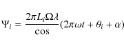
where i takes the values 1 and 2. Figure C.1 shows three modeled planet signal templates with different values of $\alpha$ and illustrates the relatively small effect on the appearance of the signal. Measured values of $\alpha$ are shown in Table 4; generally they were small.

$\begin{figure} \par\includegraphics[width=8cm]{14942fig15.eps} \par\end{figure}$	Figure C.1: Theoretical planet signals similar to those employed in these tests, showing the effect of varying $\alpha$ between $\pm$ 0.5 radian.
Open with DEXTER

References

Beichman, C. 2004, The Terrestrial Planet Finder, dSpace at Jet Propulsion Laboratory, http://trs-new.jpl.nasa.gov/dspace-oai/request (United States) [Google Scholar]
Booth, A. J., Martin, S. R., & Loya, F. 2008, in Optical and Infrared Interferometry (Marseille, France: SPIE), 7013, 20 [Google Scholar]
Bracewell, R. N. 1978, Nature, 274, 780 [NASA ADS] [CrossRef] [Google Scholar]
Cockell, C. S., Léger, A., Fridlund, M., et al. 2009, Astrobiology, 9 [Google Scholar]
Defrère, D., Absil, O., Den Hartog, R., Hanot, C., & Stark, C. 2010, AA, 509, A9 [Google Scholar]
Des Marais, D. J., Harwit, M. O., Jucks, K. W., et al. 2002, Astrobiology, 2, 153 [NASA ADS] [CrossRef] [PubMed] [Google Scholar]
Fridlund, M., Eiroa, C., Henning, T., et al. 2010, Astrobiology, 10, 5 [NASA ADS] [CrossRef] [PubMed] [Google Scholar]
Gappinger, R. O., Diaz, R. T., Ksendzov, A., et al. 2009, Appl. Opt., 48, 868 [NASA ADS] [CrossRef] [PubMed] [Google Scholar]
Kaltenegger, L., & Fridlund, M. 2005, Adv. Space Res., 36, 1114 [NASA ADS] [CrossRef] [Google Scholar]
Kaltenegger, L., Selsis, F., Fridlund, M., et al. 2010, Astrobiology, 10, 89 [NASA ADS] [CrossRef] [PubMed] [Google Scholar]
Ksendzov, A., Lay, O., Martin, S., et al. 2007, Appl. Opt., 46, 7957 [NASA ADS] [CrossRef] [PubMed] [Google Scholar]
Ksendzov, A., Lewi, T., Lay, O. P., et al. 2008, Appl. Opt., 47, 5728 [NASA ADS] [CrossRef] [PubMed] [Google Scholar]
Lane, B. F., Muterspaugh, M. W., & Shao, M. 2006, ApJ, 648, 1276 [NASA ADS] [CrossRef] [Google Scholar]
Lawson, P. R., Lay, O. P., Martin, S. R., et al. 2008, in Optical and Infrared Interferometry (Marseille, France: SPIE), 7013 [Google Scholar]
Lay, O. P. 2004, Appl. Opt., 43, 6100 [NASA ADS] [CrossRef] [PubMed] [Google Scholar]
Lay, O. P. 2006, in Advances in Stellar Interferometry (Orlando, FL, USA: SPIE), 6268 [Google Scholar]
Lay, O. P., Martin, S. R., & Hunyadi, S. L. 2007, in Techniques and Instrumentation for Detection of Exoplanets III (San Diego, CA, USA: SPIE), 6693 [Google Scholar]
Léger, A., Pirre, M., & Marceau, F. 1993, A&A, 277, 309 [NASA ADS] [Google Scholar]
Martin, S. 2005, in Techniques and Instrumentation for Detection of Exoplanets II (San Diego, CA, USA: SPIE), 5905 [Google Scholar]
Martin, S., Szwaykowski, P., & Loya, F. 2005, in Techniques and Instrumentation for Detection of Exoplanets II (San Diego, CA, USA: SPIE), 5905 [Google Scholar]
Martin, S. 2006, in Aerospace Conf., 2006 IEEE [Google Scholar]
Martin, S. 2007, in Aerospace Conf., 2007 IEEE [Google Scholar]
Martin, S. R., & Booth, A. J. 2010, A&A, 511, L1 [NASA ADS] [CrossRef] [EDP Sciences] [Google Scholar]
Mayor, M., & Queloz, D. 1995, Nature, 378, 355 [NASA ADS] [CrossRef] [Google Scholar]
Mennesson, B., & Mariotti, J. M. 1997, Icarus, 128, 202 [NASA ADS] [CrossRef] [Google Scholar]
Mennesson, B., Léger, A., & Ollivier, M. 2005, Icarus, 178, 570 [NASA ADS] [CrossRef] [Google Scholar]
Morgan, R. M., Burge, J. H., & Woolf, N. J. 2000, SPIE Conf. Ser., 4006, 340 [Google Scholar]
Peters, R. D., Lay, O. P., & Jeganathan, M. 2008, Appl. Opt., 47, 3920 [NASA ADS] [CrossRef] [PubMed] [Google Scholar]
Scharf, D., Hadaegh, F., Rahman, Z., et al. 2004, 2nd International Symp. on Formation Flying Missions and Technologies, Washington, D.C. [Google Scholar]
Scharf, D., Keim, J., & Hadaegh, F. 2010, IEEE Syst. J., 4, 84 [NASA ADS] [CrossRef] [Google Scholar]
Schindler, T. L., & Kasting, J. F. 2000, Icarus, 145, 262 [NASA ADS] [CrossRef] [MathSciNet] [PubMed] [Google Scholar]
Schneider, J., Léger, A., Fridlund, M., et al. 2010, Astrobiology, 10, 121 [NASA ADS] [CrossRef] [PubMed] [Google Scholar]
Segura, A., Meadows, V. S., Kasting, J. F., Crisp, D., & Cohen, M. 2007, AA, 472, 665 [Google Scholar]
Trauger, J. T., & Traub, W. A. 2007, Nature, 446, 771 [NASA ADS] [CrossRef] [PubMed] [Google Scholar]
Velusamy, T., Angel, R., Eatchel, A., Tenerelli, D., & Woolf, N. 2003, Proc. Towards Other Earths: DARWIN/TPF and the Search for Extrasolar Terrestrial Planets, Heidelberg, Germany, 22-25 April 2003, 631, ESA SP, 539 [Google Scholar]
Woolf, N., & Angel, R. 1997, ASP Conf. Ser., 119, 285 [NASA ADS] [Google Scholar]

Footnotes

... USA: Formerly at the Jet Propulsion Laboratory.

All Tables

Table 1: Summary of data sets taken in June and July 2009.

Table 2: Summary of data sets presented here.

Table 3: Summary of data sets presented here.

Table 4: Supplementary data reduction values.

All Figures

$\begin{figure} \par\resizebox{9cm}{!}{\includegraphics{14942fig1.eps}} \end{figure}$	Figure 1: Exoplanet detection process using a nulling interferometer.
Open with DEXTER
In the text

$\begin{figure} \par\resizebox{9cm}{!}{\includegraphics{14942fig2.eps}} \end{figure}$	Figure 2: The planet detection testbed, PDT, seen from the source end.
Open with DEXTER
In the text

$\begin{figure} \par\resizebox{9cm}{!}{\includegraphics{14942fig3.eps}} \par\end{figure}$	Figure 3: On-sky monochromatic modulation pattern for the TPF-Emma X-array. The small circle denotes the position of the star and the large circle the path traced by a planet through the fringe system as the formation rotates. The plot has been apodized to illustrate the effect of the field of view of a single mode fiber in the detection system: in reality the field of view would be a minimum of 20 fringes wide in the horizontal direction.
Open with DEXTER
In the text

$\begin{figure} \par\includegraphics[width=9cm,clip]{14942fig4.eps} \end{figure}$	Figure 4: Schematic layout of testbed beam train. Star and planet light enters from the lower left through individual synchronized choppers. Each beam is then split twice to create four beams of starlight and four of planet light. These eight beams are then combined to make four beams, one for each TPF telescope. These four beams are then passed in pairs through two nullers and thence to a cross-combiner. One output of the cross-combiner goes to a detector. Planet phases are controlled by five moving optics; four mirrors and the first planet beam splitter. The phases at the nullers are controlled similarly using a set of mirrors. Finally, the cross-combiner imposes a $\pm$ $\lambda$ /4 phase chop.
Open with DEXTER
In the text

$\begin{figure} \par\includegraphics[width=9cm,clip]{14942fig5.eps} \end{figure}$	Figure 5: Schematic layout of testbed optical systems. Only one beam path, the lowest one, is shown in its entirety since the three other beam paths have identical systems. The lines represent the light paths which travel generally from left to right. Top half of figure, the source area, the light from each source is shown being split from a single beam into four beams; A, A', A'': respectively, thermal source for planet, and laser and thermal sources for star; B, B': synchronized chopper blades; C: planet source metrology retro-reflector; D: first beam splitter in planet path, with delay line; E: first beam splitter in star path; F, F': second beam splitters; G: planet phasing mirrors; H: star-planet beam combiners (eight beams merge into four star and planet beams); J: pointing and shearing alignment laser entry point; K: planet metrology entry point. Bottom half of figure, the beam-combiner area, four beams merge into a single beam; L: intensity adjuster; M: beam combiner metrology entry point; N: pointing and shearing adjuster mirrors; Q, R: pointing and shearing sensing; P: fast and slow delay lines; S: nulling beam combiners; T: two nuller fringe tracker outputs; U: chopping cross-combiner (one beam emerges for detection); V: two cross-combiner fringe tracker outputs; W: beam combiner metrology retro-reflector; Y: spatial filter; Z: nulling detector.
Open with DEXTER
In the text

$\begin{figure} \par\includegraphics[width=9cm]{14942fig6.eps} \end{figure}$	Figure 6: Calculation of the planet phase for each beam input. The circles T represent the telescope formation rotating around the center at radii L. The phase of the planet light is measured along the bold line which passes through the star and planet.
Open with DEXTER
In the text

$\begin{figure} \par\includegraphics[width=9cm]{14942fig7.eps} \end{figure}$	Figure 7: A: the planet signal template for a planet at an angular separation of $0.635 \times 10^{-6}$ radian (130 mas) from the star, utilizing the formation parameters given in the results section. B: the corresponding correlation map on the sky when this template is tested using all the templates for planets at angular separations from $0.2 \times 10^{-7}$ radian (4 mas) to $1.75 \times 10^{-6}$ radian (360 mas). The planet's location is at the peak of the correlation at ( $6.35 \times 10^{-7}$ , 0) radian. The vertical scale of the correlation ranges from -1 (blue) to +1 (red).
Open with DEXTER
In the text

$\begin{figure} \par\includegraphics[width=9cm]{14942fig8.eps} \end{figure}$	Figure 8: The test performance data summarized in the ladder diagram form. The principal measured performance levels for the three data sets are compared with the demonstration goals. The null depth, the planet signal $\Phi$ ( $\Omega _{\rm m}$ , $\theta _{\rm m}$ ), the planet rms $\sigma _{\rm P}$ and the rms noise $\sigma _{\rm n}$ are shown compared with the normalized starlight (unity).
Open with DEXTER
In the text

$\begin{figure} \par\includegraphics[width=9cm]{14942fig9.eps} \par\end{figure}$	Figure 9: The signal processing steps shown in order for the star-only data of the 6-18 data set: A, normalized data from nulling detector, truncated to 600 000 samples, representing a 12 000 s run time. B, the data processed in synchrony with the cross-combiner chop at a 2 s period. Reset periods have been removed and the record is now 10 000 s long. C, the chopped data cyclically averaged over the five rotations; now 2000 s long. D, data (C), high-pass filtered to remove only the dc level and the first harmonic of the rotation and the reset periods.
Open with DEXTER
In the text

$\begin{figure} \par\includegraphics[width=9cm,clip]{14942fig10.eps} \end{figure}$	Figure 10: The same signal processing steps shown in order for the star and planet signal of 6-18: A, normalized data from nulling detector. B, the data processed in synchrony with the cross-combiner chop. The planet signal is already apparent. C, the chopped data cyclically averaged over the five rotations. D, data (C), high-pass filtered, showing a clear but noisy planet signal.
Open with DEXTER
In the text

$\begin{figure} \par\resizebox{15cm}{!}{\includegraphics{14942fig11.eps}} \end{figure}$	Figure 11: Summary plots normalized by the stellar intensity. A: planet-only signal data and fit. B: star-and-planet signal data and fit. C: planet-only signal, cross-correlation map of $\Phi$ in space. D: star-and-planet signal, cross-correlation map. E: star-only cross-correlation map and for comparison, F: cross-correlation map for D with the detected planet signal removed.
Open with DEXTER
In the text

$\begin{figure} \par\resizebox{16.5cm}{!}{\includegraphics{14942fig12.eps}} \end{figure}$	Figure 12: Summary plots for data of 7-10.
Open with DEXTER
In the text

$\begin{figure} \par\resizebox{17cm}{!}{\includegraphics{14942fig13.eps}} \end{figure}$	Figure 13: Summary plots for data of 7-23.
Open with DEXTER
In the text

$\begin{figure} \par\resizebox{8cm}{!}{\includegraphics{14942fig14.eps}} \end{figure}$	Figure 14: For the planet-only data of 6-18: the planet signal constructed from the planet beam train metrology data sampled at the chop frequency (blue dots) with the corresponding fitted planet signal measured from the mid-infrared detector.
Open with DEXTER
In the text

$\begin{figure} \par\includegraphics[width=8cm]{14942fig15.eps} \par\end{figure}$	Figure C.1: Theoretical planet signals similar to those employed in these tests, showing the effect of varying $\alpha$ between $\pm$ 0.5 radian.
Open with DEXTER
In the text

Current usage metrics show cumulative count of Article Views (full-text article views including HTML views, PDF and ePub downloads, according to the available data) and Abstracts Views on Vision4Press platform.

Data correspond to usage on the plateform after 2015. The current usage metrics is available 48-96 hours after online publication and is updated daily on week days.

Initial download of the metrics may take a while.

[1] Beichman, C. 2004, The Terrestrial Planet Finder, dSpace at Jet Propulsion Laboratory, http://trs-new.jpl.nasa.gov/dspace-oai/request (United States) [Google Scholar]

[2] Booth, A. J., Martin, S. R., & Loya, F. 2008, in Optical and Infrared Interferometry (Marseille, France: SPIE), 7013, 20 [Google Scholar]

[3] Bracewell, R. N. 1978, Nature, 274, 780 [NASA ADS] [CrossRef] [Google Scholar]

[4] Cockell, C. S., Léger, A., Fridlund, M., et al. 2009, Astrobiology, 9 [Google Scholar]

[5] Defrère, D., Absil, O., Den Hartog, R., Hanot, C., & Stark, C. 2010, AA, 509, A9 [Google Scholar]

[6] Des Marais, D. J., Harwit, M. O., Jucks, K. W., et al. 2002, Astrobiology, 2, 153 [NASA ADS] [CrossRef] [PubMed] [Google Scholar]

[7] Fridlund, M., Eiroa, C., Henning, T., et al. 2010, Astrobiology, 10, 5 [NASA ADS] [CrossRef] [PubMed] [Google Scholar]

[8] Gappinger, R. O., Diaz, R. T., Ksendzov, A., et al. 2009, Appl. Opt., 48, 868 [NASA ADS] [CrossRef] [PubMed] [Google Scholar]

[9] Kaltenegger, L., & Fridlund, M. 2005, Adv. Space Res., 36, 1114 [NASA ADS] [CrossRef] [Google Scholar]

[10] Kaltenegger, L., Selsis, F., Fridlund, M., et al. 2010, Astrobiology, 10, 89 [NASA ADS] [CrossRef] [PubMed] [Google Scholar]

[11] Ksendzov, A., Lay, O., Martin, S., et al. 2007, Appl. Opt., 46, 7957 [NASA ADS] [CrossRef] [PubMed] [Google Scholar]

[12] Ksendzov, A., Lewi, T., Lay, O. P., et al. 2008, Appl. Opt., 47, 5728 [NASA ADS] [CrossRef] [PubMed] [Google Scholar]

[13] Lane, B. F., Muterspaugh, M. W., & Shao, M. 2006, ApJ, 648, 1276 [NASA ADS] [CrossRef] [Google Scholar]

[14] Lawson, P. R., Lay, O. P., Martin, S. R., et al. 2008, in Optical and Infrared Interferometry (Marseille, France: SPIE), 7013 [Google Scholar]

[15] Lay, O. P. 2004, Appl. Opt., 43, 6100 [NASA ADS] [CrossRef] [PubMed] [Google Scholar]

[16] Lay, O. P. 2006, in Advances in Stellar Interferometry (Orlando, FL, USA: SPIE), 6268 [Google Scholar]

[17] Lay, O. P., Martin, S. R., & Hunyadi, S. L. 2007, in Techniques and Instrumentation for Detection of Exoplanets III (San Diego, CA, USA: SPIE), 6693 [Google Scholar]

[18] Léger, A., Pirre, M., & Marceau, F. 1993, A&A, 277, 309 [NASA ADS] [Google Scholar]

[19] Martin, S. 2005, in Techniques and Instrumentation for Detection of Exoplanets II (San Diego, CA, USA: SPIE), 5905 [Google Scholar]

[20] Martin, S., Szwaykowski, P., & Loya, F. 2005, in Techniques and Instrumentation for Detection of Exoplanets II (San Diego, CA, USA: SPIE), 5905 [Google Scholar]

[21] Martin, S. 2006, in Aerospace Conf., 2006 IEEE [Google Scholar]

[22] Martin, S. 2007, in Aerospace Conf., 2007 IEEE [Google Scholar]

[23] Martin, S. R., & Booth, A. J. 2010, A&A, 511, L1 [NASA ADS] [CrossRef] [EDP Sciences] [Google Scholar]

[24] Mayor, M., & Queloz, D. 1995, Nature, 378, 355 [NASA ADS] [CrossRef] [Google Scholar]

[25] Mennesson, B., & Mariotti, J. M. 1997, Icarus, 128, 202 [NASA ADS] [CrossRef] [Google Scholar]

[26] Mennesson, B., Léger, A., & Ollivier, M. 2005, Icarus, 178, 570 [NASA ADS] [CrossRef] [Google Scholar]

[27] Morgan, R. M., Burge, J. H., & Woolf, N. J. 2000, SPIE Conf. Ser., 4006, 340 [Google Scholar]

[28] Peters, R. D., Lay, O. P., & Jeganathan, M. 2008, Appl. Opt., 47, 3920 [NASA ADS] [CrossRef] [PubMed] [Google Scholar]

[29] Scharf, D., Hadaegh, F., Rahman, Z., et al. 2004, 2nd International Symp. on Formation Flying Missions and Technologies, Washington, D.C. [Google Scholar]

[30] Scharf, D., Keim, J., & Hadaegh, F. 2010, IEEE Syst. J., 4, 84 [NASA ADS] [CrossRef] [Google Scholar]

[31] Schindler, T. L., & Kasting, J. F. 2000, Icarus, 145, 262 [NASA ADS] [CrossRef] [MathSciNet] [PubMed] [Google Scholar]

[32] Schneider, J., Léger, A., Fridlund, M., et al. 2010, Astrobiology, 10, 121 [NASA ADS] [CrossRef] [PubMed] [Google Scholar]

[33] Segura, A., Meadows, V. S., Kasting, J. F., Crisp, D., & Cohen, M. 2007, AA, 472, 665 [Google Scholar]

[34] Trauger, J. T., & Traub, W. A. 2007, Nature, 446, 771 [NASA ADS] [CrossRef] [PubMed] [Google Scholar]

[35] Velusamy, T., Angel, R., Eatchel, A., Tenerelli, D., & Woolf, N. 2003, Proc. Towards Other Earths: DARWIN/TPF and the Search for Extrasolar Terrestrial Planets, Heidelberg, Germany, 22-25 April 2003, 631, ESA SP, 539 [Google Scholar]

[36] Woolf, N., & Angel, R. 1997, ASP Conf. Ser., 119, 285 [NASA ADS] [Google Scholar]