| Issue |
A&A
Volume 520, September-October 2010
|
|
|---|---|---|
| Article Number | A92 | |
| Number of page(s) | 5 | |
| Section | Planets and planetary systems | |
| DOI | https://doi.org/10.1051/0004-6361/201014761 | |
| Published online | 08 October 2010 | |
Global plasma-parameter simulation of
Comet 67P/Churyumov-Gerasimenko approaching the Sun![[*]](/icons/foot_motif.png)
N. Gortsas1 - U. Motschmann1,2 - E. Kührt1 - K.-H. Glassmeier3,4 - K. C. Hansen5 - J. Müller2 - A. Schmidt6
1 - Institute for Planetary Research, German Aerospace Center (DLR),
Rutherfordstr. 2, 12489 Berlin, Germany
2 - Institute for Theoretical Physics, TU Braunschweig,
Mendelssohnstrasse 3, 38106 Braunschweig, Germany
3 - Institute for Geophysics und Extraterrestrial Physics,
Mendelssohnstrasse 3, 38106 Braunschweig, Germany
4 - Max-Planck-Institute for Solar System Research, Max-Planck-Str. 2,
37191 Katlenburg-Lindau, Germany
5 - Department of Atmospheric, Oceanic and Space Sciences, The
University of Michigan, Ann Arbor, Michigan 48109-2143, USA
6 - European Space Astronomy Centre, PO Box 78, 28691 Villanueva de la
Caada (Madrid), Spain
Received 9 April 2010 / Accepted 27 July 2010
Abstract
We simulate the evolution of the plasma environment of comet
67P/Churyumov-Gerasimenko (CG), which is the target comet of the
European Space Agency's (ESA) Rosetta mission, as the comet approaches
the Sun.
The plasma environment is calculated in three dimensions with a hybrid
plasma model.
The model treats the dynamics of the solar wind protons and the
cometary ions in the framework of the macroparticle approach while
the electrons are treated as a massless, charge-neutralizing
fluid. The simulation starts at 4.2 AU and finishes at
1.3 AU.
The outgassing strength of the comet is calculated from a
thermal nucleus model. The model accounts for heat conduction, heat
advection, gas
diffusion, sublimation, and condensation processes in
a porous ice-dust matrix with moving boundaries. The movement
of the boundaries (Stefan problem) is accounted for by a temperature
remapping technique.
The maxima of the cometary ion flux and of the magnetic field in the
simulation domain are presented as functions of heliocentric distance.
The bow shock (BS), the ion composition boundary (ICB), and the
magnetic pileup boundary (MPB) position along the Sun-comet line as a
function of
heliocentric distance are also discussed. A comparison of the BS
position with an analytical formula yields good agreement. The MPB and
the ICB along the Sun-comet line coincide.
Key words: comets: general - comets: individual: 67P/Churyumov-Gerasimenko - plasmas - magnetic fields - interplanetary medium - methods: numerical
1 Introduction
We simulate the plasma environment of comet 67P/Churyumov-Gerasimenko (CG), which is the target of the European Space Agency's (ESA) Rosetta mission (Glassmeier et al. 2007), during its journey into the inner Solar System by combining a hybrid plasma simulation model with a thermophysical nucleus model. This combined effort allows us a unique insight into the evolution of the plasma environment of a weak comet with increasing activity (Coates & Jones 2009).
A key input parameter of the hybrid plasma model is the outgassing strength of the comet. In the present investigation the major cometary ion species is considered, i.e. water group ions. The outgassing strength is calculated from a sophisticated nucleus model that treats different processes such as heat conduction, heat advection, gas diffusion, sublimation, and condensation with moving boundaries in a chemically diverse nucleus. For a review of the efforts in the field of thermophysical modeling of comet nuclei we refer the reader to Prialnik et al. (2004) and the reference therein. Previous articles concerning the plasma environment of comets were performed at some fixed heliocentric distances and the outgassing strength was set to an estimated number based on observations, or else it was derived from a simple outgassing model (Gortsas et al. 2009; Lipatov et al. 2002; Motschmann & Kührt 2006; Delamere 2006). One of the first studies of the dynamic and very complex phenomenon of a comet approaching the Sun and thereby gaining strength in its outgassing of volatile materials has been presented by Bagdonat & Motschmann (2002). The authors studied the plasma environment of comet 46P/Wirtanen for several heliocentric distances between 3.25 AU to 1 AU in 2D and 3D. Based on characteristic plasma structures, different interaction regimes were identified. An improved investigation was presented by Hansen et al. (2007), who applied the hybrid plasma model of Bagdonat & Motschmann (2002) and the MHD model of Gombosi et al. (1996) to investigate the plasma environment of CG at four fixed heliocentric distances. This investigation has shown that important insight in to the plasma environment of comets is obtained through a kinetic approach as presented in the hybrid plasma model. Especially far from perihelion a kinetic description reveals important aspects of the solar-wind/comet interaction.
The novel feature of this study is the sophisticated thermal model employed to calculate the water activity of CG and the quasi continuous simulation of the cometary approach to perihelion. The simulation starts at 4.2 AU and finishes at 1.3 AU with a step size in heliocentric direction of 0.1 AU. In the presentation of the simulation results strong emphasis is laid on the evolution of the cometary ion flux and the magnetic field compared to the undisturbed solar wind and the interplanetary magnetic field. The simulation results are compared with analytical formulas for the BS standoff distance. Scaling laws of important boundaries are also presented.
![\begin{figure}
\par\includegraphics[width=9cm,clip]{14761fig1.eps}
\end{figure}](/articles/aa/full_html/2010/12/aa14761-10/img6.png)
|
Figure 1: Left scale: maximum of the cometary ion flux as a function of heliocentric distance. The maximum is taken from the whole simulation domain and fitted with a rational law r-1.4. For comparison the undisturbed solar wind ion flux is also shown. Three regimes can be distinguished. At the beginning, the solar-wind ion flux exceeds the cometary ion flux, this is the test-particle regime that covers the range from 4.2 AU to 3.7 AU. Around 3.7 AU, these quantities reach the same values. This regime is referred to as the Mach cone regime, which covers the range up to 2.7 AU. From 2.7 AU to 1.3 AU, the maximum cometary ion flux clealry exceeds the solar wind ion flux. This is the shock formation regime. Right scale: total water outgassing rates. |
| Open with DEXTER | |
2 Simulation model and input parameters
We apply a three-dimensional, quasi-neutral hybrid plasma model to study the evolution of the plasma environment of CG as the comet approaches the Sun. The dynamics of the solar wind protons and the cometary ions are described in the framework of the macroparticle approach while the electrons are treated as a massless, charge-neutralizing fluid. The key features of the hybrid model are discussed in preceding publications (Gortsas et al. 2009; Bagdonat & Motschmann 2002). Therefore, only a brief overview of the main aspects for this study shall be given.
We start the calculation at 4.2 AU from scratch.
After the simulation has reached quasi-stationarity, the result is
taken
as the starting point of the simulation at 4.1 AU. This is
continued until
perihelion. At each heliocentric distance the solar wind passes the
simulation box up to
five times. The dependence of the solar wind environment parameters,
e.g. solar wind background density n0
and the strength of the interplanetary magnetic
field ![]() ,
are obtained through a fit of Voyager 2 and IMP 8 data (Richardson et al. 1995)
and with the Parker model (Parker 1958).
The corresponding curves are shown in Fig. 1 for the solar-wind
ion flux
and in Fig. 2
for the magnetic field strength.
The increasing outgassing strength of the comet makes it necessary to
adapt the size of the simulation box. This is done in a trial-and-error
fashion with
the aim to keep the characteristic plasma structures like bow shock
approximately
in the middle of the simulation box and to get a smooth transition
between
adjacent steps. The simulation domain increases from 1200 km
at 4.2 AU to 24 000 km at perihelion.
,
are obtained through a fit of Voyager 2 and IMP 8 data (Richardson et al. 1995)
and with the Parker model (Parker 1958).
The corresponding curves are shown in Fig. 1 for the solar-wind
ion flux
and in Fig. 2
for the magnetic field strength.
The increasing outgassing strength of the comet makes it necessary to
adapt the size of the simulation box. This is done in a trial-and-error
fashion with
the aim to keep the characteristic plasma structures like bow shock
approximately
in the middle of the simulation box and to get a smooth transition
between
adjacent steps. The simulation domain increases from 1200 km
at 4.2 AU to 24 000 km at perihelion.
![\begin{figure}
\par\includegraphics[width=12cm,clip]{14761fig2.eps} \vspace*{4mm}
\end{figure}](/articles/aa/full_html/2010/12/aa14761-10/img7.png)
|
Figure 2:
Maximum of the magnetic field as function of heliocentric distance is
shown. The maximum is taken from the whole simulation domain and fitted
with a rational law of r-0.5.
For comparison the interplanetary magnetic field is also depicted. As
the comet approaches the Sun the magnetic field maximum exceeds the
|
| Open with DEXTER | |
The outgassing pattern in the hybrid code is spherically symmetric
and the outgassing strength is derived from a further development of
the thermophysical nucleus model of Kührt
(1999). The model consists of water ice, CO ice, and dust in
a porous ice-dust matrix. It solves the coupled heat
and mass transfer problem with moving boundary conditions. The model
takes into account erosion due to surface sublimation, which leads
to the loss of internal energy stored in the eroded subsurface layers.
This is achieved by applying the so-called temperature remapping
technique. Following the work of Crank
& Gupta (1972) the spatial discretization is kept
constant
while the grid is moved according to the amount of surface sublimation.
The thickness of the eroded surface layers ![]() is calculated from the Stefan condition (Stefan
1891)
is calculated from the Stefan condition (Stefan
1891)

Q denotes the amount of surface sublimation of water
ice, ![]() is the difference in thermal enthalpy, and
is the difference in thermal enthalpy, and ![]() the mass density of water ice.
In extension to that, a non-constant number of intervals
is introduced in order to be able to calculate oscillating boundaries,
which can come very close to the surface. This adaptive approach is
essential to model cometary activity of a multi-component nucleus. More
details of the
nucleus model will be published in an upcoming article.
the mass density of water ice.
In extension to that, a non-constant number of intervals
is introduced in order to be able to calculate oscillating boundaries,
which can come very close to the surface. This adaptive approach is
essential to model cometary activity of a multi-component nucleus. More
details of the
nucleus model will be published in an upcoming article.
3 Simulation results
3.1 Global view of the solar wind-comet interaction
Part of this manuscript is a movie showing the absolute value
of
cometary ion flux and of the magnetic field in
the orthogonal plane of ![]() as the comet approaches
the Sun. The movie is available as an online supplement.
as the comet approaches
the Sun. The movie is available as an online supplement.
The simulation results for the water-outgassing strength are
displayed in Fig. 1.
The water sublimation curve is fitted to observations of Schleicher (2006) by
integrating over the whole nucleus and by assuming that 3![]() of the total surface is active.
At 4.2 AU the comet is very faint, reaching an integrated
water activity of 1024 s-1.
At these large heliocentric distances water activity is very low.
But other more volatile species can sublime from the nucleus despite
low energy input from the Sun.
Such a volatile species would be CO. For the present investigation,
however, only water vapor is considered in the hybrid plasma model.
Depending on the simulation parameters of the thermal model
water exceeds CO-outgassing between 4 AU to 3.5 AU.
Therefore, the role of CO is not
further investigated here. At perihelion, the comet reaches a
water-outgassing strength of
of the total surface is active.
At 4.2 AU the comet is very faint, reaching an integrated
water activity of 1024 s-1.
At these large heliocentric distances water activity is very low.
But other more volatile species can sublime from the nucleus despite
low energy input from the Sun.
Such a volatile species would be CO. For the present investigation,
however, only water vapor is considered in the hybrid plasma model.
Depending on the simulation parameters of the thermal model
water exceeds CO-outgassing between 4 AU to 3.5 AU.
Therefore, the role of CO is not
further investigated here. At perihelion, the comet reaches a
water-outgassing strength of
![]() s-1.
Thus, during the simulation cometary water activity
increases by more then three orders of magnitude.
s-1.
Thus, during the simulation cometary water activity
increases by more then three orders of magnitude.
The weak outgassing strength at 4.2 AU yields a
maximum value of the cometary ion
flux, which is one order of magnitude below the undisturbed solar
wind ion flux as displayed in Fig. 1. At around
3.7 AU, cometary
activity has increased and yields a maximum ion flux that is comparable
to the undisturbed solar-wind ion flux. The evolution of the magnetic
field is depicted in Fig. 2.
At the beginning, the maximum of the magnetic field is a factor
of 2.5 above the ![]() .
This value is reached in front of the nucleus, while farther away the
magnetic field remains undisturbed. At 3.7 AU this factor
rises to a value of almost 5. The interval starting at
4.2 AU to 3.7 AU exhibits features which are
characteristic to the test-particle regime as described in Bagdonat & Motschmann (2002).
The comet is too faint to cause any
significant feedback to the solar wind.
.
This value is reached in front of the nucleus, while farther away the
magnetic field remains undisturbed. At 3.7 AU this factor
rises to a value of almost 5. The interval starting at
4.2 AU to 3.7 AU exhibits features which are
characteristic to the test-particle regime as described in Bagdonat & Motschmann (2002).
The comet is too faint to cause any
significant feedback to the solar wind.
![\begin{figure}
\par\includegraphics[width=9cm,clip]{14761fig3.eps} \vspace*{2mm}
\end{figure}](/articles/aa/full_html/2010/12/aa14761-10/img14.png)
|
Figure 3:
Left scale: the distance of the bow shock
(BS), the magnetic pileup boundary (MPB), and the ion composition
boundary (ICB) to the nucleus along the Sun-comet line is displayed.
The BS position agrees well with an analytical formula of Galeev et al. (1985).
The MPB and the ICB are well fitted by
|
| Open with DEXTER | |
The simulation data allow us to identify a second regime that covers a
heliocentric range from 3.7 AU to 2.7 AU. In this
interval, the growth of cometary activity is about 2 to 3 orders of
magnitude. This growth process is followed by the cometary ion flux,
which exceeds
the solar wind flux by a factor of 2 at the end of the interval.
The magnetic field exceeds the
![]() by a factor of 7. Compared to the factor
at 3.7 AU this amounts to a moderate enhancement of
about 1.4.
This regime has been characterized in previous studies of the
solar-wind/comet interaction by the
formation of the linear Mach cone (Lipatov et al. 2002; Bagdonat
& Motschmann 2002).
by a factor of 7. Compared to the factor
at 3.7 AU this amounts to a moderate enhancement of
about 1.4.
This regime has been characterized in previous studies of the
solar-wind/comet interaction by the
formation of the linear Mach cone (Lipatov et al. 2002; Bagdonat
& Motschmann 2002).
The last regime spans the distance from 2.7 AU to 1.3 AU. In this interval, cometary activity increases by more than one order of magnitude. The maximum of the cometary ion flux and of the magnetic field, however, seem to grow only moderately. Both quantities exceed the background values of the solar wind by a factor of 2 and 7, respectively; factors that were already reached at 2.7 AU. Hence, despite the growth in cometary activity by one order of magnitude, the maximum of the magnetic field and the cometary ion flux seem to follow the growth of the interplanetary magnetic field strength and the solar wind ion flux. In previous investigations of the solar-wind/comet interaction this last regime was characterized by the splitting of the Mach cone and the formation of a bow shock (Bagdonat & Motschmann 2002).
The proposed division of the simulation range in three interaction regimes appears to agree well with the investigation of Hansen et al. (2007). There are also differences though. The test-particle regime is farther away from the Sun in the ranges from 4.2 AU to 3.7 AU, while in Hansen et al. (2007) this regime was at 3.25 AU. This is mainly because of different water-outgassing curves. The formation of the Mach cone was identified by Hansen et al. (2007) at 2.7 AU, which coincides well with the present investigation. According to the present simulation the Mach cone evolves between 3.4 AU to 2.7 AU. In the global view of the solar wind-comet interaction the splitting of the Mach cone and the formation of the bow shock cannot be separated. These structures evolve from 2.7 AU to perihelion. As the comet approaches its perihelion position, the Hansen et al. (2007) and the present investigation converge as the differences in the employed water activity get smaller.
3.2 Shocks and cometary characteristics
The position of the bow shock ![]() relative to the comet as function
of heliocentric distance is compared with an analytical formula derived
by Biermann et al. (1967).
Assuming a stationary flow in an axial-symmetric 1 D model of the solar
wind
the mass flux equation reads (Biermann
et al. 1967)
relative to the comet as function
of heliocentric distance is compared with an analytical formula derived
by Biermann et al. (1967).
Assuming a stationary flow in an axial-symmetric 1 D model of the solar
wind
the mass flux equation reads (Biermann
et al. 1967)
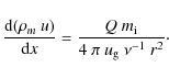
Integrating this equation from the undisturbed solar wind conditions to the location of the bow shock leads to the following expression for the standoff distance
![\begin{displaymath}
R_{\rm bs} = \frac{Q ~ m_{\rm i}}{4~ \pi ~ u_{\rm g} ~ \nu^...
...\infty} ~ u_{\infty} [ (\hat{\rho}~\hat{u})_{\rm c} -1]} \cdot
\end{displaymath}](/articles/aa/full_html/2010/12/aa14761-10/img17.png)
![]() ,
,
![]() ,
,![]() ,
,
![]() ,
and
,
and ![]() denote the cometary ion mass of the water species, the escape velocity
of the ions, e.g. 1 km s-1,
the ionization
rate, e.g. 10-6 s-1,
the background solar-wind proton-mass density, and velocity.
denote the cometary ion mass of the water species, the escape velocity
of the ions, e.g. 1 km s-1,
the ionization
rate, e.g. 10-6 s-1,
the background solar-wind proton-mass density, and velocity.
![]() denotes
the critical mass flux ratio of the contaminated solar wind
for shock formation. A continuous solar wind flow is possible only
until
the point at which the mean molecular weight of the solar wind
particles reaches
a critical value. This value was estimated by Biermann
et al. (1967)
to be
denotes
the critical mass flux ratio of the contaminated solar wind
for shock formation. A continuous solar wind flow is possible only
until
the point at which the mean molecular weight of the solar wind
particles reaches
a critical value. This value was estimated by Biermann
et al. (1967)
to be ![]() based on a simplified one-dimensional model.
Schmidt & Wegmann (1982)
showed that for 1P/Halley at 1 AU a shock wave with Mach
number 2 occurred at
a distance from the nucleus where
based on a simplified one-dimensional model.
Schmidt & Wegmann (1982)
showed that for 1P/Halley at 1 AU a shock wave with Mach
number 2 occurred at
a distance from the nucleus where ![]() .
Huddleston et al. (1992)
employed Eq. (3)
under the assumption that
the critical number
.
Huddleston et al. (1992)
employed Eq. (3)
under the assumption that
the critical number ![]() is mainly a function of the cometary
ion flux, while the solar wind ion flux is set to the undisturbed
background values
far from the comet. The authors obtained estimates for the shock
position
along the Sun-comet line in the range of
is mainly a function of the cometary
ion flux, while the solar wind ion flux is set to the undisturbed
background values
far from the comet. The authors obtained estimates for the shock
position
along the Sun-comet line in the range of ![]() km
for comet 26P/Grigg-Skjellerup
with a
km
for comet 26P/Grigg-Skjellerup
with a ![]() value of 1.22. In the present investigation, the critical value
value of 1.22. In the present investigation, the critical value ![]() is used as a fit parameter. It turns out that the hybrid
simulation data of the standoff distance are well fitted by
Eq. (3)
if
is used as a fit parameter. It turns out that the hybrid
simulation data of the standoff distance are well fitted by
Eq. (3)
if ![]() has a value of 2.05. At perihelion, the standoff distance
of CG is
has a value of 2.05. At perihelion, the standoff distance
of CG is ![]() km,
which is a factor of 2 below the value of comet 26P/Grigg-Skjellerup,
which has almost the same outgassing strength as CG at perihelion.
km,
which is a factor of 2 below the value of comet 26P/Grigg-Skjellerup,
which has almost the same outgassing strength as CG at perihelion.
The standoff distance of the bow shock, the position of the
ion composition boundary,
and the magnetic pile-up boundary as function of heliocentric distance
are displayed
in Fig. 3
from 2 AU to perihelion because these boundaries are not well
defined beyond 2 AU. The outgassing strength of the nucleus is
too low beyond 2 AU. The ICB is defined as the location of the
cross point along the Sun-comet line
of the solar-wind proton density and the cometary ion density.
The position of the MPB is represented by the peak value of the
magnetic field strength.
The ICB and MPB coincide well at perihelion, while farther away from
the Sun these
boundaries appear to follow different patterns. The ICB follows a r-0.3
fit while the MPB a r-0.56
fit. The latter is comparable to the fit of the maximum magnetic field
in the simulation domain of
![]() as
presented in Fig. 2.
The coincidence of the ICB and the MPB at comet CG has also been
observed at planet Mars by Bösswetter
et al. (2004). The fit to the cometary ion flux
maximum shown in Fig. 1
is
as
presented in Fig. 2.
The coincidence of the ICB and the MPB at comet CG has also been
observed at planet Mars by Bösswetter
et al. (2004). The fit to the cometary ion flux
maximum shown in Fig. 1
is ![]() .
A summary of the fit laws can be found in Table 1.
.
A summary of the fit laws can be found in Table 1.
Table 1: Scaling laws.
In Fig. 3 we also display the bow shock strength in terms of the Mach number as function of heliocentric distance. One can see that the hybrid model predicts a BS with a Mach number of about 2.3 for comet CG. As the comet approaches its perihelion position, the Mach number of the solar wind flow drops very steeply to this value.
4 Conclusion
We investigate the evolution of the plasma environment of comet CG as the comet approaches the Sun. The simulations are performed by combining two different and sophisticated models. We calculate the plasma environment with the quasi-neutral, three dimensional hybrid plasma model. The outgassing strength of the comet, an important input parameter of the hybrid plasma model, is calculated from a thermophysical nucleus model. The thermal model solves the coupled heat- and mass transfer problem in a porous ice-dust matrix with moving boundaries (Stefan problem).
The simulation starts at 4.2 AU and finishes at 1.3 AU with a step size in heliocentric distance of 0.1 AU. The maximum of the cometary ion flux and of the magnetic field are presented as functions of heliocentric distance. As part of this investigation a movie is published, which shows the perihelion approach of CG for the cometary ion flux and the magnetic field.
The simulation results allow us to distinguish three different
regimes.
The test-particle regime covers a heliocentric distance between
4.2 AU to 3.7 AU. Weak mass-loading of the solar wind
leads to
a moderate enhancement of the magnetic field, which is localized
in the vicinity of the nucleus and which reaches factors in the range
2.5 to 5 compared to the ![]() .
In the Mach cone regime which covers a heliocentric distance of
3.7 AU to about 2.7 AU, the cometary ion flux exceeds
the undisturbed solar-wind ion flow and leads to
a stronger feedback on the solar wind parameters. The magnetic field
exhibits an enhancement by a factor 7, which is detached from
the nucleus surface. The last regime
covers a distance of 2.7 AU to perihelion. Although this
regime
shows strong effects on the plasma environment of the comet, the
absolute
values of the magnetic field and the cometary ion flux appear
to follow the growth process of the interplanetary magnetic field
and of the solar-wind ion flux as the comet approaches the Sun.
.
In the Mach cone regime which covers a heliocentric distance of
3.7 AU to about 2.7 AU, the cometary ion flux exceeds
the undisturbed solar-wind ion flow and leads to
a stronger feedback on the solar wind parameters. The magnetic field
exhibits an enhancement by a factor 7, which is detached from
the nucleus surface. The last regime
covers a distance of 2.7 AU to perihelion. Although this
regime
shows strong effects on the plasma environment of the comet, the
absolute
values of the magnetic field and the cometary ion flux appear
to follow the growth process of the interplanetary magnetic field
and of the solar-wind ion flux as the comet approaches the Sun.
The position of the bow shock along the Sun-comet line is compared with an analytical formula by Biermann et al. (1967) and Galeev et al. (1985), which agree well.
We also presented rational law fits to the hybrid simulation data. Fits to the maximum of the cometary ion flux, the maximum of the magnetic field magnitude, and fits along the Sun-comet line to the MPB, the ICB, and the BS position as function of heliocentric distance are discussed. The hybrid model predicts a BS with a Mach number of about 2.3. With decreasing heliocentric distance the Mach number drops very steeply.
AcknowledgementsThe authors are indebted to the ISSI comet modeling team for fruitful discussions. The work of U.M. and J.M. was supported by the Deutsche Forschungsgemeinschaft under grant number MO 539/16-1. The work by K.H.G. was financially supported by the Deutsches Zentrum für Luft- und Raumfahrt and the Bundesministerium für Wirtschaft und Technologie under grant 50 QP 0402.
References
- Bagdonat, T., & Motschmann, U. 2002, Earth Moon and Planets, 90, 305 [NASA ADS] [CrossRef] [Google Scholar]
- Biermann, L., Brosowski, B., & Schmidt, H. U. 1967, Sol. Phys., 1, 254 [NASA ADS] [CrossRef] [Google Scholar]
- Bösswetter, A., Bagdonat, T., Motschmann, U., & Sauer, K. 2004, Ann. Geophys., 22, 4363 [Google Scholar]
- Coates, A. J., & Jones, G. H. 2009, Planet Space Sci., 57, 1175 [CrossRef] [Google Scholar]
- Crank, J., & Gupta, R. S. 1972, J. Inst. Math. Appl., 10, 296 [CrossRef] [Google Scholar]
- Delamere, P. A. 2006, J. Geophys. Res., 111, 12217 [CrossRef] [Google Scholar]
- Galeev, A. A., Cravens, T. E., & Gombosi, T. I. 1985, ApJ, 289, 807 [NASA ADS] [CrossRef] [Google Scholar]
- Glassmeier, K., Boehnhardt, H., Koschny, D., Kührt, E., & Richter, I. 2007, Space Sci. Rev., 128, 1 [NASA ADS] [CrossRef] [Google Scholar]
- Gombosi, T. I., De Zeeuw, D. L., Häberli, R. M., & Powell, K. G. 1996, J. Geophys. Res., 101, 15233 [NASA ADS] [CrossRef] [Google Scholar]
- Gortsas, N., Motschmann, U., KÃijhrt, E., et al. 2009, Ann. Geophys., 27, 1555 [NASA ADS] [CrossRef] [Google Scholar]
- Hansen, K. C., Bagdonat, T., Motschmann, U., et al. 2007, Space Sci. Rev., 128, 133 [NASA ADS] [CrossRef] [Google Scholar]
- Huddleston, D. E., Coates, A. J., & Johnstone, A. D. 1992, Geophys. Res. Lett., 19, 837 [NASA ADS] [CrossRef] [Google Scholar]
- Kührt, E. 1999, Space Sci. Rev., 90, 75 [NASA ADS] [CrossRef] [Google Scholar]
- Lipatov, A. S., Motschmann, U., & Bagdonat, T. 2002, Planet Space. Sci., 50, 403 [NASA ADS] [CrossRef] [Google Scholar]
- Motschmann, U., & Kührt, E. 2006, Space Sci. Rev., 122, 197 [NASA ADS] [CrossRef] [Google Scholar]
- Parker, E. N. 1958, ApJ, 128, 664 [Google Scholar]
- Prialnik, D., Benkhoff, J., & Podolak, M. 2004, Modeling the structure and activity of comet nuclei, ed. Festou, M. C., Keller, H. U., & Weaver, H. A., 359 [Google Scholar]
- Richardson, J. D., Paularena, K. I., Lazarus, A. J., & Belcher, J. W. 1995, Geophys. Res. Lett., 22, 325 [NASA ADS] [CrossRef] [Google Scholar]
- Schleicher, D. G. 2006, Icarus, 181, 442 [CrossRef] [Google Scholar]
- Schmidt, H. U., & Wegmann, R. 1982, in Comet Discoveries, Statistics, and Observational Selection, ed. L. L. Wilkening, IAU Colloq., 61, 538 [Google Scholar]
- Stefan, J. 1891, Ann. Phys. Chem., 42, 269 [Google Scholar]
Online Material
Download the movie: hybrid_67P_movie.wmv.
Footnotes
- ... Sun
- A movie showing the plasma environment of CG during its approach to the Sun is available in electronic form at http://www.aanda.org.
All Tables
Table 1: Scaling laws.
All Figures
|
|
Figure 1: Left scale: maximum of the cometary ion flux as a function of heliocentric distance. The maximum is taken from the whole simulation domain and fitted with a rational law r-1.4. For comparison the undisturbed solar wind ion flux is also shown. Three regimes can be distinguished. At the beginning, the solar-wind ion flux exceeds the cometary ion flux, this is the test-particle regime that covers the range from 4.2 AU to 3.7 AU. Around 3.7 AU, these quantities reach the same values. This regime is referred to as the Mach cone regime, which covers the range up to 2.7 AU. From 2.7 AU to 1.3 AU, the maximum cometary ion flux clealry exceeds the solar wind ion flux. This is the shock formation regime. Right scale: total water outgassing rates. |
| Open with DEXTER | |
| In the text | |
|
|
Figure 2:
Maximum of the magnetic field as function of heliocentric distance is
shown. The maximum is taken from the whole simulation domain and fitted
with a rational law of r-0.5.
For comparison the interplanetary magnetic field is also depicted. As
the comet approaches the Sun the magnetic field maximum exceeds the
|
| Open with DEXTER | |
| In the text | |
|
|
Figure 3:
Left scale: the distance of the bow shock
(BS), the magnetic pileup boundary (MPB), and the ion composition
boundary (ICB) to the nucleus along the Sun-comet line is displayed.
The BS position agrees well with an analytical formula of Galeev et al. (1985).
The MPB and the ICB are well fitted by
|
| Open with DEXTER | |
| In the text | |
Copyright ESO 2010
Current usage metrics show cumulative count of Article Views (full-text article views including HTML views, PDF and ePub downloads, according to the available data) and Abstracts Views on Vision4Press platform.
Data correspond to usage on the plateform after 2015. The current usage metrics is available 48-96 hours after online publication and is updated daily on week days.
Initial download of the metrics may take a while.