| Issue |
A&A
Volume 520, September-October 2010
|
|
|---|---|---|
| Article Number | A32 | |
| Number of page(s) | 18 | |
| Section | Planets and planetary systems | |
| DOI | https://doi.org/10.1051/0004-6361/201014208 | |
| Published online | 24 September 2010 | |
The Edgeworth-Kuiper debris disk
Ch. Vitense - A. V. Krivov - T. Löhne
Astrophysikalisches Institut, Friedrich-Schiller-Universität Jena, Schillergäßchen 2-3, 07745 Jena, Germany
Received 5 February 2010 / Accepted 8 June 2010
Abstract
The Edgeworth-Kuiper belt (EKB) and its presumed dusty debris is
a natural reference for extrsolar debris disks.
We re-analyze the current database of known transneptunian objects
(TNOs)
and employ a new algorithm to eliminate the inclination and the
distance selection
effects in the known TNO populations to derive expected
parameters of the ``true'' EKB.
Its estimated mass is
![]() ,
which is by a factor of
,
which is by a factor of ![]() 15
larger than the mass
of the EKB objects detected so far.
About a half of the total EKB mass is in classical and resonant
objects and another half is in scattered ones.
Treating the debiased populations
of EKB objects as dust parent bodies, we then ``generate'' their dust
disk
with our collisional code.
Apart from accurate handling of
destructive and cratering collisions and direct radiation pressure, we
include the Poynting-Robertson (P-R) drag.
The latter is known to be
unimportant for debris disks around other stars detected so far, but
cannot
be ignored for the EKB dust disk because of its much lower optical
depth.
We find the radial profile of the normal optical depth to peak
at the inner edge of the classical belt,
15
larger than the mass
of the EKB objects detected so far.
About a half of the total EKB mass is in classical and resonant
objects and another half is in scattered ones.
Treating the debiased populations
of EKB objects as dust parent bodies, we then ``generate'' their dust
disk
with our collisional code.
Apart from accurate handling of
destructive and cratering collisions and direct radiation pressure, we
include the Poynting-Robertson (P-R) drag.
The latter is known to be
unimportant for debris disks around other stars detected so far, but
cannot
be ignored for the EKB dust disk because of its much lower optical
depth.
We find the radial profile of the normal optical depth to peak
at the inner edge of the classical belt, ![]()
![]() .
Outside the classical EKB, it approximately follows
.
Outside the classical EKB, it approximately follows
![]() which is roughly intermediate
between the slope
predicted analytically for collision-dominated (r-1.5)
and transport-dominated (r-2.5)
disks.
The size distribution of dust is less affected by the P-R effect.
The cross section-dominating grain size still lies just above
the blowout size (
which is roughly intermediate
between the slope
predicted analytically for collision-dominated (r-1.5)
and transport-dominated (r-2.5)
disks.
The size distribution of dust is less affected by the P-R effect.
The cross section-dominating grain size still lies just above
the blowout size (![]()
![]() ),
as it would if the P-R effect was ignored.
However, if the EKB were by one order of magnitude less massive, its
dust disk would have
distinctly different properties. The optical depth profile would fall
off
as
),
as it would if the P-R effect was ignored.
However, if the EKB were by one order of magnitude less massive, its
dust disk would have
distinctly different properties. The optical depth profile would fall
off
as ![]() ,
and
the cross section-dominating grain size would shift from
,
and
the cross section-dominating grain size would shift from ![]()
![]() to
to
![]()
![]() .
These properties are seen if dust is assumed to be generated only by
known TNOs
without applying the debiasing algorithm.
An upper limit of the in-plane optical depth of the EKB dust set by our
model
is
.
These properties are seen if dust is assumed to be generated only by
known TNOs
without applying the debiasing algorithm.
An upper limit of the in-plane optical depth of the EKB dust set by our
model
is ![]() outside
outside ![]() .
If the solar system were observed from outside, the thermal emission
flux from the EKB dust
would be about two orders of magnitude lower than for
solar-type stars with the brightest known infrared excesses observed
from the same distance.
Herschel and other new-generation facilities should reveal extrasolar
debris disks
nearly as tenuous as the EKB disk.
We estimate that the Herschel/PACS instrument should be able to detect
disks at a
.
If the solar system were observed from outside, the thermal emission
flux from the EKB dust
would be about two orders of magnitude lower than for
solar-type stars with the brightest known infrared excesses observed
from the same distance.
Herschel and other new-generation facilities should reveal extrasolar
debris disks
nearly as tenuous as the EKB disk.
We estimate that the Herschel/PACS instrument should be able to detect
disks at a ![]()
![]() level.
level.
Key words: Kuiper belt: general - methods: statistical - methods: numerical - planetary systems - circumstellar matter - infrared: planetary systems
1 Introduction
Debris disks, now known to be ubiquitous around main-sequence stars, are the natural aftermath of the evolution of dense protoplanetary disks that may or may not result in formation of planets (see, e.g., Krivov 2010; Wyatt 2008, for recent reviews). They are composed of left-over planetesimals and smaller debris produced in mutual collisions, and it is the tiniest, dust-sized collisional fragments that are evident in observations through thermal radiation and scattered stellar light.
Like planetary systems of other stars, our solar system contains planetesimals that have survived planetary formation. The main asteroid belt between two groups of planets, terrestrial and giant ones, comprises planetesimals that failed to grow to planets because of the strong perturbations by the nearby Jupiter (e.g., Wetherill 1980; Safronov 1969). The Edgeworth-Kuiper Belt (EKB) exterior to the Neptune orbit is built up by planetesimals that did not form planets because the density of the outer solar nebula was too low (e.g., Lissauer 1987; Kenyon & Bromley 2008; Safronov 1969). Both the asteroid belt and the Kuiper belt are heavily structured dynamically, predominantly by Jupiter and Neptune respectively. They include non-resonant and resonant families, as well as various objects in transient orbits ranging from detached and scattered Kuiper-belt objects through Centaurs to Sun-grazers. Short-period comets, another tangible population of small bodies in the inner solar system, must be genetically related to the Kuiper belt that acts as their reservoir (Quinn et al. 1990). Asteroids and short-period comets together are sources of interplanetary dust, observed in the planetary region, although their relative contribution to the dust production remain uncertain (Grün et al. 2001). And this complex system structure was likely quite different in the past. It is argued that the giant planets and the Kuiper belt have originally formed in a more compact configuration (the ``Nice model'', Gomes et al. 2005), and that it went through a short-lasting period of dynamical instability, likely explaining the geologically recorded event of the Late Heavy Bombardment (LHB).
As the amount of material and spatial dimensions of the EKB surpass by far those of the asteroid belt and the population of short-period comets, it is the EKB and its presumed collisional debris that should be referred to as the debris disk of the solar system. Ironically, the observational status of the solar system's debris disk is the opposite of that of the debris disks around other stars. In the latter case, as mentioned above, it is dust that can be observed. In the former case, we can observe the planetesimals, but there is no certain detection of their dust so far (Landgraf et al. 2002; Gurnett et al. 1997).
An obvious difference between the debris disks detected so far around other stars and our solar system's debris disk is the total mass (and thus, also the amount of dust). Müller et al. (2010) for example infer several Earth masses as the total mass of the Vega debris disk, whereas the Kuiper belt mass is reported to be below one-tenth of the Earth mass (Bernstein et al. 2004; Fuentes & Holman 2008). As a result, were the solar system observed from afar, its debris dust would be far below the detection limits. However, a number of debris disks around Sun-like stars that are coeval with or even older than the Sun have been detected. Booth et al. (2009) analyze ``dusty consequences'' of a major depletion of the planetesimal populations in the solar system at the LHB phase. They point out that the pre-LHB debris disk of the Sun would be among the brightest debris disks around solar-type stars currently observed. Future, more sensitive observations (for instance, with Herschel Space Observatory) should detect lower-mass disks, bridging the gap between dusty debris disks around other stars and tenous debris disks in the present-day solar system.
Given the low mass of the dust parent bodies in the EKB, our debris disk is thought to fall into the category of the so-called transport-dominated disks (Krivov et al. 2000), where radial transport timescales for dust (due to the Poynting-Robertson effect, henceforth P-R, e.g. Burns et al. 1979) are shorter than their collisional lifetime. This is opposite to extrasolar debris disks that are collision-dominated (Wyatt 2005). Whereas the latter have been extensively modeled both analytically and numerically (Thébault & Augereau 2007; Müller et al. 2010; Thébault et al. 2003; Krivov et al. 2006; Strubbe & Chiang 2006; Löhne et al. 2008; Wyatt et al. 2007), more effort has to be invested into modeling of transport-dominated disks. The more so, as new-generation facilities like Herschel Space Observatory will soon open a phase when low-density, transport-dominated disks can be studied observationally.
The main goal of this paper is to develop a more realistic model of such a tenuous disk, exemplified by the EKB dust disk, than was done before (e.g. Stern 1995). We take an advantage that - unlike with other debris disks and unlike at the time when the first collisional models of the EKB dust were devised - more than a thousand EKB objects, acting as dust parent bodies of the solar system's debris disk, are now known. This task is accomplished in two steps:
- I.
- first, the currently known objects in the EKB are analyzed. In Sect. 2, we work out an algorithm to correct their distributions for observational selection effects and try to reconstruct the properties of the expected ``true'' EKB;
- II.
- second, we treat the objects of the ``true'' EKB as dust parent bodies. In Sect. 3, we make simulations of dust production and evolution with a statistical code, fully taking into account collisions and the P-R effect, and present the expected radial and size distribution of the presumed EKB dust. In Sect. 4, we model the spectral energy distribution (SED) of the simulated EKB dust disk and compare it to the SEDs of other debris disks. We also compare these results with the detection limits of the Herschel/PACS instrument.
2 Planetesimals in the Kuiper belt
2.1 Observations and their biases
The EKB was predicted more than fifty years ago by Edgeworth and Kuiper
and it took fourty
years until the first object, QB 1, was discovered (Jewitt et al. 1992).
More than 1260 transneptunian objects (TNOs) orbiting the Sun beyond
the orbit of Neptune have been discovered.
Table 1
lists most of the surveys published so far, in which new TNOs
have been discovered, and key parameters of these surveys.
One parameter is the area ![]() on the sky searched for TNOs.
Another one is the limiting magnitude m50that
corresponds to the detection probability of
on the sky searched for TNOs.
Another one is the limiting magnitude m50that
corresponds to the detection probability of ![]() .
As the detection probability drops rapidly from 100% to zero when the
apparent magnitude m ``crosses'' m50,
we simply assume that an object
will be detected with certainty if
m
< m50 and missed
otherwise.
Finally, the maximum ecliptic latitude
.
As the detection probability drops rapidly from 100% to zero when the
apparent magnitude m ``crosses'' m50,
we simply assume that an object
will be detected with certainty if
m
< m50 and missed
otherwise.
Finally, the maximum ecliptic latitude
![]() covered by each survey is listed.
Where it was not given explicitly in the original papers, we estimated
it
to be
covered by each survey is listed.
Where it was not given explicitly in the original papers, we estimated
it
to be ![]() ,
assuming
that the surveyed area was centered on the ecliptic.
Table 1
shows that all campaigns
can be roughly divided into two groups:
deeper ones with a small sky area covered (``pencil-beam'' surveys)
and shallower ones with a larger area, but a smaller limiting
magnitude.
,
assuming
that the surveyed area was centered on the ecliptic.
Table 1
shows that all campaigns
can be roughly divided into two groups:
deeper ones with a small sky area covered (``pencil-beam'' surveys)
and shallower ones with a larger area, but a smaller limiting
magnitude.
Table 1: A list of campaigns where TNOs were found.
The orbits of TNOs are commonly characterized by
six orbital elements:
semi-major axis a(or perihelion
distance q),
eccentricity e,
inclination i,
argument of pericenter ![]() ,
longitude of the ascending node
,
longitude of the ascending node ![]() ,
and mean anomaly M.
In addition, each object itself is characterized by the absolute
magnitude H, which is defined as the
apparent magnitude the object would have if it was
,
and mean anomaly M.
In addition, each object itself is characterized by the absolute
magnitude H, which is defined as the
apparent magnitude the object would have if it was
![]() away from the Sun and the Earth, and depends on the object radius and
albedo.
We take the orbital elements and the absolute magnitudes of all known
objects
from the Minor Planet Center (MPC) database
away from the Sun and the Earth, and depends on the object radius and
albedo.
We take the orbital elements and the absolute magnitudes of all known
objects
from the Minor Planet Center (MPC) database![]() rather than from discovery papers listed in Table 1,
because the MPC data include follow-up observations and thus provide
a better precision.
rather than from discovery papers listed in Table 1,
because the MPC data include follow-up observations and thus provide
a better precision.
![\begin{figure}
\par\includegraphics[width=17cm]{14208fig1.eps}
\end{figure}](/articles/aa/full_html/2010/12/aa14208-10/img41.png)
|
Figure 1:
Known TNOs in the a-e plane
(top) and a-i plane (bottom).
Different groups are shown with different symbols:
865 classical objects with dots, 235 resonant TNOs
with pluses, and the remaining 160 scattered objects with
crosses. Solid lines separate classical and scattered objects in our
classification. One object with
|
| Open with DEXTER | |
The planet formation theory implies that the TNO orbits strongly
concentrate
towards the ecliptic plane.
Accordingly, in order to increase the detection probability,
the majority of the observations were made near the ecliptic, and only
a few
surveys covered high ecliptic latitudes.
Our sample, given in Table 1,
contains surveys with ![]() up to
up to ![]() (e.g.
Elliot
et al. 2005; Trujillo & Brown 2003;
Trujillo
et al. 2001a; Petit et al. 2006;
Larsen
et al. 2007).
However, TNOs with higher orbital inclinations exist as well.
Since Brown (2001) it is
known that the inclination distribution of TNOs
has a second maximum at higher inclinations.
Several objects with very high inclinations, including one with
(e.g.
Elliot
et al. 2005; Trujillo & Brown 2003;
Trujillo
et al. 2001a; Petit et al. 2006;
Larsen
et al. 2007).
However, TNOs with higher orbital inclinations exist as well.
Since Brown (2001) it is
known that the inclination distribution of TNOs
has a second maximum at higher inclinations.
Several objects with very high inclinations, including one with
![]() ,
were detected.
Clearly, the fact that observations are done near the ecliptic plane
decreases
the probability to detect such objects, because it is only possible
twice per orbital period, close to the nodes.
Thus there is an obvious selection effect in favor of TNOs in
low-inclination orbits
that needs to be taken into account.
Equally obvious is another selection effect, which is that objects are
predominantly
discovered at smaller heliocentric distances. This reduces the
probability to
discover TNOs with large semi-major axes and high eccentricities,
because these are too faint all the time except for the short period of
time when they are near perihelion.
,
were detected.
Clearly, the fact that observations are done near the ecliptic plane
decreases
the probability to detect such objects, because it is only possible
twice per orbital period, close to the nodes.
Thus there is an obvious selection effect in favor of TNOs in
low-inclination orbits
that needs to be taken into account.
Equally obvious is another selection effect, which is that objects are
predominantly
discovered at smaller heliocentric distances. This reduces the
probability to
discover TNOs with large semi-major axes and high eccentricities,
because these are too faint all the time except for the short period of
time when they are near perihelion.
2.2 Classification of TNOs
Many classifications of TNOs into ``classical'', ``resonant'', ``excited'', ``scattered'', ``detached'' etc. groups have been proposed, based on the orbital elements and taking into account dynamical arguments (e.g., Jewitt et al. 1998; Chiang & Brown 1999; Jewitt et al. 2009; Delsanti & Jewitt 2006; Luu & Jewitt 2002, among others). Classifications by different authors are similar, but not identical. In this paper we use the following working classification:
- 1.
- resonant objects (RES): objects in a mean-motion
commensurability with Neptune, where we only consider the three most
prominent first-order resonances 4:3, 3:2 and 2:1. To identify the
objects as resonant, we use the resonance ``widths'' from Murray & Dermott (2000).
For example, the width of the 3:2-resonance at e=0.1
is
 .
The width increases with increasing eccentricity and with decreasing
distance to Neptune;
.
The width increases with increasing eccentricity and with decreasing
distance to Neptune; - 2.
- classical Kuiper Belt (CKB) objects: objects with
 ,
which are
neither resonant nor Neptune-crossers (
,
which are
neither resonant nor Neptune-crossers (
 );
); - 3.
- scattered disk objects (SDO): objects with
 ,
as well as Neptune-crossers (
,
as well as Neptune-crossers (
 and
and
 ).
).
2.3 Debiasing procedure
Because of the obvious selection effects of inclined and faint objects, statistical models were developed to estimate a true distribution of orbital elements and numbers of the TNOs. Brown (2001) calculated an inclination distribution. He assumed circular orbits and derived a relation between the inclination and the fraction of an object's orbit that it spends at low ecliptic latitudes. Donnison (2006) calculated the magnitude distribution for the classical, resonant, and scattered objects for absolute magnitudes H<7, using maximum likelihood estimations, and showed that the samples were statistically different.
Here we propose another debiasing method to estimate the
``true''
distribution of the TNOs, based on the obervational surveys listed in
Table 1.
We start with calculating the probability to find an
object with the given parameters
![]() for each given
survey.
To this end, we estimate the time fraction of the object's orbit that
lies within
the maximum ecliptic latitude
for each given
survey.
To this end, we estimate the time fraction of the object's orbit that
lies within
the maximum ecliptic latitude
![]() covered by the survey, as
well as the fraction of the orbit which is observable at the given
limiting
magnitude m50, and
find the intersection of the two orbital arcs. Once
the probability to detect the object in each of the surveys has been
calculated, we compute the probability that it would be detected at
least
in one of the surveys made so far.
Finally, we augment the number of objects with that same orbital
elements
as the object considered to a
covered by the survey, as
well as the fraction of the orbit which is observable at the given
limiting
magnitude m50, and
find the intersection of the two orbital arcs. Once
the probability to detect the object in each of the surveys has been
calculated, we compute the probability that it would be detected at
least
in one of the surveys made so far.
Finally, we augment the number of objects with that same orbital
elements
as the object considered to a ![]() probability, e.g., an
object with
probability, e.g., an
object with ![]() probability is counted five times.
probability is counted five times.
We now explain this procedure in more detail. The first effect
is the ``inclination bias''. In calculating the
orbital arc that lies in the
observable latitudinal zone, we make the assumption that we observe
from the sun.
The observable area on the sky is thus a belt
![]() ,
where b is
the heliocentric ecliptic latitude.
The orbit crosses the boundary of the observed belt,
,
where b is
the heliocentric ecliptic latitude.
The orbit crosses the boundary of the observed belt,
![]() ,
at four points. At these intersection points, the true anomaly
,
at four points. At these intersection points, the true anomaly ![]() takes
the values
takes
the values
Due to our approximation that we observe from the Sun, the longitude of the ascending node does not appear in this formula.
The second effect is the ``distance bias''
(or ``eccentricity
bias''). The maximum distance at which an object is
detectable is given by
Irwin et al. (1995)

Then we combine both observability constraints, from inclination (Eq. (1)) and eccentricity (Eq. (2)), into one, to find the orbital arc (or arcs) that lie both in the observable latitudinal belt and the observable sphere. Typical geometries are sketched in Fig. 2, assuming that the pericenter is inside the observing latitudinal belt. The intersection points of the orbit with the visibility sphere
As an example, we take ellipse number III. The object starts at the pericenter (where it is visible) and moves toward I1. Between I1 and I2, it is outside the observed latitudinal belt and is invisible. Although it has a sufficiently low ecliptic latitude up to I3, it is only detectable up to E1, because it gets too faint beyond that point. Between I3 and I4 the object is too far from from the ecliptic, and it stays outside the limiting sphere until it reaches E2. Starting from E2, the object is visible again.
![\begin{figure}
\par\mbox{\includegraphics[width=0.16\textwidth]{14208fig2a.eps} ...
...g2h.eps} \includegraphics[width=0.16\textwidth]{14208fig2i.eps} }
\end{figure}](/articles/aa/full_html/2010/12/aa14208-10/img61.png)
|
Figure 2:
Observable arc(s) of a TNO orbit that satisfy the distance and the
inclination restrictions. Smaller points denoted with E1
and E2 are intersection
points of the orbit with the sphere
|
| Open with DEXTER | |
In this way, for each of the known TNOs,
we can calculate the detection probability in any survey.
We then calculate the probability Pi
that an object iwould be detected in any of
the ![]() surveys:
surveys:
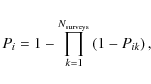
where Pik is the probability to detect an object i in a survey k. The advantage of Eq. (3) is that 1-Pik gives the probability not to detect an object, ``shallower'' surveys make little contribution to the product and thus to the total detection probability of very faint objects. Therefore, it is deep surveys that dominate the result for faint objects.
Given the discovery probability Pi of a given object, we can augment the observed Kuiper belt to the ``true'' one by counting that object Pi-1 times. In other words, we debias the observed Kuiper belt by setting the number of TNOs with the same orbital elements as the known object to Pi-1.
The number of surveys in Table 1 is
![]() .
However, only nearly half of the 1260 TNOs contained in the
MPC database were found in these campaigns.
Another
.
However, only nearly half of the 1260 TNOs contained in the
MPC database were found in these campaigns.
Another ![]() 600 objects
were discovered in other observations, some
serendipitously in surveys that did not aim to search for TNOs.
The circumstances of those observations have not been been published in
all cases.
What is more, even for the campaigns listed in Table 1,
it is problematic to identify which particular set of
600 objects
were discovered in other observations, some
serendipitously in surveys that did not aim to search for TNOs.
The circumstances of those observations have not been been published in
all cases.
What is more, even for the campaigns listed in Table 1,
it is problematic to identify which particular set of ![]() 600 objects
out of 1260 in total was found in those surveys.
Indeed, the papers that give a specific, identifiable list of newly
discovered objects
(marked with an asterisk in Table 1) only
cover
600 objects
out of 1260 in total was found in those surveys.
Indeed, the papers that give a specific, identifiable list of newly
discovered objects
(marked with an asterisk in Table 1) only
cover ![]() 400 TNOs.
We do not know under which
circumstances the remaining two-thirds of the TNOs were detected.
In other words, there is no guarantee that the parameters of those
unknown surveys (m50,
400 TNOs.
We do not know under which
circumstances the remaining two-thirds of the TNOs were detected.
In other words, there is no guarantee that the parameters of those
unknown surveys (m50,
![]() etc.) are similar to those listed in
Table 1.
Furthermore, some of the surveys
in our list may not have reported their discoveries to the MPC.
As a result, it is difficult to judge how complete the MPC database is.
We can even suspect that there have been surveys not listed in
Table 1
that have
discovered TNOs not listed in the MPC.
Therefore, it does not appear possible to compile a complete version of
Table 1
that would cover all known TNOs and
all discovery observations (together with their
etc.) are similar to those listed in
Table 1.
Furthermore, some of the surveys
in our list may not have reported their discoveries to the MPC.
As a result, it is difficult to judge how complete the MPC database is.
We can even suspect that there have been surveys not listed in
Table 1
that have
discovered TNOs not listed in the MPC.
Therefore, it does not appear possible to compile a complete version of
Table 1
that would cover all known TNOs and
all discovery observations (together with their ![]() ,
m50, and
,
m50, and
![]() ).
Nor is it possible to get a complete list of all known TNOs together
with their orbital elements, along with information in which
particular survey each of the known TNOs was discovered.
To cope with these difficulties,
we make two assumptions.
First, we assume that the surveys listed in
Table 1
are representative of all surveys that discovered TNOs.
Second, we assume that, conversely, the TNOs listed is the
MPC are respresentative of all the objects discovered in surveys
listed in Table 1.
These two assumptions represent the main
shortcoming of our debiasing approach.
).
Nor is it possible to get a complete list of all known TNOs together
with their orbital elements, along with information in which
particular survey each of the known TNOs was discovered.
To cope with these difficulties,
we make two assumptions.
First, we assume that the surveys listed in
Table 1
are representative of all surveys that discovered TNOs.
Second, we assume that, conversely, the TNOs listed is the
MPC are respresentative of all the objects discovered in surveys
listed in Table 1.
These two assumptions represent the main
shortcoming of our debiasing approach.
To check them at least partly and proceed with the debiasing,
we employed two different methods.
In the first method, we have randomly chosen 600 TNOs out of
the full list of known
objects and assumed that it is these objects that were discovered in
the campaigns
listed in Table 1.
We tried this several times for different
sets of 600 TNOs and found that the results (e.g., the
elemental distributions and the total mass of the ``debiased EKB'') are
in close agreement.
In the second method, we have made an assumption that another set of
23 similar surveys with similar detection success rate would
have likely led to a discovery of all known TNOs. So we simply counted
each survey twice and replaced Eq. (3) by
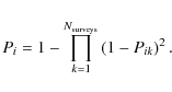
Again, the results turned out to be very close to those found with the first method.
Figure 3
illustrates
the probabilities Pik
to observe known TNOs
in a fiducial survey with
![]() ,
a latitudinal coverage of
,
a latitudinal coverage of
![]() ,
and a longitudinal coverage of
,
and a longitudinal coverage of ![]() .
Let us start with an artificial case where all objects are in circular
orbits.
If they were bright enough to be observed
(or equivalently, in the limiting case
.
Let us start with an artificial case where all objects are in circular
orbits.
If they were bright enough to be observed
(or equivalently, in the limiting case
![]() ),
they would all lie on the curve overplotted in Fig. 3.
In particular, their detection probability would be 100%
for
),
they would all lie on the curve overplotted in Fig. 3.
In particular, their detection probability would be 100%
for ![]() ,
and it would be
,
and it would be
![]() %
for
%
for ![]() .
If they are too faint for detection, their detection probability will
be zero
regardless of the inclination.
The case of eccentric orbits is more complicated.
Then, the vast majority objects still are on the curve but, as seen in
the figure,
there are many that lie below.
Either these are objects whose pericenter is outside of the latitudinal
belt
.
If they are too faint for detection, their detection probability will
be zero
regardless of the inclination.
The case of eccentric orbits is more complicated.
Then, the vast majority objects still are on the curve but, as seen in
the figure,
there are many that lie below.
Either these are objects whose pericenter is outside of the latitudinal
belt ![]() or these are objects that cannot be observed over the entire orbits,
even when they have sufficiently low ecliptic latitude,
because in some low-latitude parts of their orbits they are too faint
to be visible.
In fact, a mixture of both cases is typical.
Finally, a few objects lie above the curve.
These are rare cases of objects in highly-eccentric orbits,
whose aphelia fall into the observable latitudinal belt,
and whose apocentric distances are not too large.
Such objects spend much of their orbital period near aphelia and are
detectable there,
which raises their detection probability.
or these are objects that cannot be observed over the entire orbits,
even when they have sufficiently low ecliptic latitude,
because in some low-latitude parts of their orbits they are too faint
to be visible.
In fact, a mixture of both cases is typical.
Finally, a few objects lie above the curve.
These are rare cases of objects in highly-eccentric orbits,
whose aphelia fall into the observable latitudinal belt,
and whose apocentric distances are not too large.
Such objects spend much of their orbital period near aphelia and are
detectable there,
which raises their detection probability.
![\begin{figure}
\par\includegraphics[width=8.8cm]{14208fig3.eps}
\end{figure}](/articles/aa/full_html/2010/12/aa14208-10/img73.png)
|
Figure 3:
The detection probability of all known TNOs (as function of their
orbital inclinations) in a fiducial survey with a full coverage of a
belt on the sky within
|
| Open with DEXTER | |
Although the average detection probability in Fig. 3
is quite high, this only holds for a complete coverage of the
![]() band on the sky.
In reality, only a limited range of the ecliptic longitude is covered.
The resulting detection probability Pi
of all known TNOs in all 23 surveys,
calculated with Eq. (4)
that takes into account actual
latitudinal coverage of the observational campaigns,
is plotted in Fig. 4.
Typical values are within
band on the sky.
In reality, only a limited range of the ecliptic longitude is covered.
The resulting detection probability Pi
of all known TNOs in all 23 surveys,
calculated with Eq. (4)
that takes into account actual
latitudinal coverage of the observational campaigns,
is plotted in Fig. 4.
Typical values are within ![]() 20%
for near-ecliptic orbits and drop to a few percent for inclinations
above
20%
for near-ecliptic orbits and drop to a few percent for inclinations
above ![]() .
.
![\begin{figure}
\par\includegraphics[width=8.8cm]{14208fig4.eps}
\end{figure}](/articles/aa/full_html/2010/12/aa14208-10/img74.png)
|
Figure 4: The final detection probability of the known TNOs, calculated with Eq. (4). Included are all surveys from Table 1. |
| Open with DEXTER | |
2.4 Orbital element distributions of the Kuiper belt objects
Having applied the debiasing procedure, we compared and analyzed the distributions of orbital elements of the known and the ``true'' EKB - separately for each class.
Figures 5
and 6
show the distributions
in terms of numbers (for ![]() )
and
masses (for
)
and
masses (for ![]() )
of objects per element's bin before and after debiasing.
The distribution in terms of numbers
depicted in Fig. 5
emphasizes smaller, more numerous, TNOs.
It is directly related to observational counts of TNOs and is also
useful to alleviate comparison with similar work by the others.
In contrast, the distribution of TNO's mass in Fig. 6 is
dominated by
larger objects. It demonstrates more clearly where the wealth of the
EKB material
is located, which aids placing the EKB in context of extrasolar debris
disks.
Objects with
)
of objects per element's bin before and after debiasing.
The distribution in terms of numbers
depicted in Fig. 5
emphasizes smaller, more numerous, TNOs.
It is directly related to observational counts of TNOs and is also
useful to alleviate comparison with similar work by the others.
In contrast, the distribution of TNO's mass in Fig. 6 is
dominated by
larger objects. It demonstrates more clearly where the wealth of the
EKB material
is located, which aids placing the EKB in context of extrasolar debris
disks.
Objects with ![]() were excluded from Fig. 5, because
detections of the smallest objects are the least complete,
which would lead to a highly uncertain, distorted distribution.
And conversely, we excluded the biggest objects with
were excluded from Fig. 5, because
detections of the smallest objects are the least complete,
which would lead to a highly uncertain, distorted distribution.
And conversely, we excluded the biggest objects with
![]() from
Fig 6
to avoid large bin-to-bin variations stemming
from a few individual rogues. Failure to do this would lead, for
example, to
a pronounced peak in the eccentricity distribution of resonant objects
at
from
Fig 6
to avoid large bin-to-bin variations stemming
from a few individual rogues. Failure to do this would lead, for
example, to
a pronounced peak in the eccentricity distribution of resonant objects
at ![]() produced by
a single object, Pluto.
produced by
a single object, Pluto.
As seen in Figs. 5 and 6 for the
classical Kuiper belt,
debiasing increases the total number and mass of objects, but the
position of the maximum remains at
![]() .
The same holds for the semimajor axis distribution of resonant objects,
whose
peaks are preserved at known resonant locations.
In contrast, for the scattered objects, here are indications that a
substantial unbiased
population with larger semimajor axes of
.
The same holds for the semimajor axis distribution of resonant objects,
whose
peaks are preserved at known resonant locations.
In contrast, for the scattered objects, here are indications that a
substantial unbiased
population with larger semimajor axes of
![]() might exist.
Some of them may be ``detached'' (
might exist.
Some of them may be ``detached'' (
![]() ), while some others
may not (since the eccentricities of these TNOs are also large, see
middle panels in the bottom rows of Figs. 5 and 6).
These conclusions should be taken with caution,
because the statistics of scattered objects is scarce and their
debiasing factors are the largest.
), while some others
may not (since the eccentricities of these TNOs are also large, see
middle panels in the bottom rows of Figs. 5 and 6).
These conclusions should be taken with caution,
because the statistics of scattered objects is scarce and their
debiasing factors are the largest.
The eccentricity distribution in Figs. 5 and 6
shows moderate values (e<0.2) for the
classical belt and reveals a broad maximum at
![]() for the resonant objects.
The maximum for the scattered objects appears to be located around
for the resonant objects.
The maximum for the scattered objects appears to be located around
![]() .
.
As far as the inclination distribution (right panels in
Figs. 5
and 6)
is concerned,
our analysis confirms the result by Brown
(2001) who indentified two
distinct subpopulations in the classical Kuiper belt, a cold one with
low
inclinations and a hot one with more inclined orbits.
The maxima of ![]() and
and
![]() that we found are consistent
with his results of
that we found are consistent
with his results of
![]() and
and
![]() .
.
The inclination distribution of the resonant objects
reveals a broad maximum around ![]()
![]() .
For comparison, Brown (2001)
found a
maximum at
.
For comparison, Brown (2001)
found a
maximum at
![]() .
A second maximum visible at
.
A second maximum visible at
![]() in
the number distribution (Fig. 5) is due to
small objects
with a large debiasing factor, which are still
big enough not to fall under the
in
the number distribution (Fig. 5) is due to
small objects
with a large debiasing factor, which are still
big enough not to fall under the
![]() criterion.
That is why in Fig. 6
the same
peak is barely seen.
criterion.
That is why in Fig. 6
the same
peak is barely seen.
A clear difference between the number and mass distributions
can be seen in the
bottom right panels of the two figures, too, which show the inclination
distribution
of the scattered objects.
A large number of scattered TNOs can be found at
![]() (Fig. 5),
whereas their mass peaks at
(Fig. 5),
whereas their mass peaks at
![]() (Fig. 6).
Interestingly, a recent paper by Gulbis
et al. (2010) yielded
(Fig. 6).
Interestingly, a recent paper by Gulbis
et al. (2010) yielded
![]() ,
which is
close to the maxima we find here.
,
which is
close to the maxima we find here.
![\begin{figure}
\par\includegraphics[width=17cm]{14208fig5.eps}
\end{figure}](/articles/aa/full_html/2010/12/aa14208-10/img96.png)
|
Figure 5:
Distribution of classical (top row), resonant (middle
row), and scattered objects (bottom row),
in terms of numbers of objects. Left column:
semimajor axes, middle: eccentricities,
right: inclinations. Black and grey bars in each panel
represent the expected (unbiased) and observed populations,
respectively. The numbers of the observed TNOs are magnified
by 20 (classical and resonant objects) and 50
(scattered objects) for better visibility. Numbers are given
in 1000 for intervals with a width of
|
| Open with DEXTER | |
![\begin{figure}
\par\includegraphics[width=17cm]{14208fig6.eps}
\end{figure}](/articles/aa/full_html/2010/12/aa14208-10/img97.png)
|
Figure 6: Same as Fig. 5, but in terms of mass contained in TNOs. |
| Open with DEXTER | |
2.5 Albedos and sizes of the Kuiper belt objects
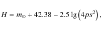
To estimate the TNO sizes, we employed the V-band
formula from
Kavelaars et al.
(2009):
|
(5) |
where

With this equation and albedo measurements from Stansberry et al. (2008); Noll et al. (2004); Brucker et al. (2009), we calculated the radius of objects with known albedo (Fig. 7).
Albedos inferred for a handful of big objects with ![]() turned out
to be high, which is indicative of a strongly reflecting surface
material.
For instance, the surface of Haumea was found to be covered with
>
turned out
to be high, which is indicative of a strongly reflecting surface
material.
For instance, the surface of Haumea was found to be covered with
>![]() pure
water ice (Pinilla-Alonso
et al. 2009).
Dumas et al. (2007)
reported for Eris
pure
water ice (Pinilla-Alonso
et al. 2009).
Dumas et al. (2007)
reported for Eris ![]() methane ice on its surface
along with nitrogen and water ices, and ice tholin.
Smaller objects are coated with darker carbonaceous layers,
so their albedo is lower.
Note that objects between 6<H<7 have a
very strong
scatter, the reason for that being unknown. Albedos of the smallest
TNOs with 7<H<9 are typically close to
methane ice on its surface
along with nitrogen and water ices, and ice tholin.
Smaller objects are coated with darker carbonaceous layers,
so their albedo is lower.
Note that objects between 6<H<7 have a
very strong
scatter, the reason for that being unknown. Albedos of the smallest
TNOs with 7<H<9 are typically close to
![]() 0.05,
and there have been no measurements beyond H=9.
However, since the EKB is known to act as a reservoir of short-period
comets,
we can use the measurements of cometary nuclei with sizes
of
0.05,
and there have been no measurements beyond H=9.
However, since the EKB is known to act as a reservoir of short-period
comets,
we can use the measurements of cometary nuclei with sizes
of ![]() 1-
1-
![]() as a proxy for the reflectance
properties of
the smallest TNOs. (The obvious caveat is that comets may have altered
their original surface properties as a result of their long residence
in the inner solar system.)
The typical albedo values of the nuclei
range from 0.02 to 0.06 (Lamy
et al. 2004).
as a proxy for the reflectance
properties of
the smallest TNOs. (The obvious caveat is that comets may have altered
their original surface properties as a result of their long residence
in the inner solar system.)
The typical albedo values of the nuclei
range from 0.02 to 0.06 (Lamy
et al. 2004).
On these grounds, to eliminate the dependence on albedo (which
is not known for most of the Kuiper belt objects) from Eq. (6),
we have fitted the sizes of the TNOs with known albedo
by an exponential function at H < 6and
assumed p=0.05 for all TNOs with ![]() .
This yielded a formula where s is only a function
of H:
.
This yielded a formula where s is only a function
of H:
and
The smallest object found so far is a scattered object with
![\begin{figure}
\par\includegraphics[width=9cm]{14208fig7.eps} \vspace*{-1.5mm}
\end{figure}](/articles/aa/full_html/2010/12/aa14208-10/img112.png)
|
Figure 7:
Absolute magnitude - radius relation for objects with known albedo. The
biggest objects are labeled with their names. The thick solid line is a
fit to this relation, Eqs. (7)-(8). Thin lines
correspond to equal albedos of
|
| Open with DEXTER | |
2.6 Mass of the Kuiper belt
To translate the TNO sizes into mass requires assumptions for the bulk
density.
We took the commonly used value of
![]() .
This assumption is in accord with the values of
.
This assumption is in accord with the values of
![]() found
for a few individual TNOs (Lacerda
2009).
The resulting mass and number of objects in resonant, classical, and
scattered populations and in the entire Kuiper belt are listed in
Table 2.
The deduced ``true'' masses are several times higher
than in Fuentes &
Holman (2008) who inferred
found
for a few individual TNOs (Lacerda
2009).
The resulting mass and number of objects in resonant, classical, and
scattered populations and in the entire Kuiper belt are listed in
Table 2.
The deduced ``true'' masses are several times higher
than in Fuentes &
Holman (2008) who inferred
![]() ,
,
![]() ,
with a total
of
,
with a total
of
![]() .
However, they considered the mass within
.
However, they considered the mass within ![]()
![]() around
the ecliptic.
Since we investigated the full range of ecliptic latitudes, we deem the
results consistent with each other.
around
the ecliptic.
Since we investigated the full range of ecliptic latitudes, we deem the
results consistent with each other.
Table 2: Masses and numbers of objects in the Kuiper belt.
One issue about the deduced mass of the entire EKB and its
populations
is the influence of the uncertainties of the orbital elements inferred
from
the observations. In many cases, the elements are known only roughly,
and some of them are not known at all. For 134 out of 865
known
classical objects, for instance, the observed arc was so short
that a circular orbit was assumed by the observers (these objects are
clearly visible as an e=0 stripe in the upper panel
of Fig. 1).
How could a change in the orbital elements of an object affect the
debiasing procedure
and the final estimates of the parameters of the ``true'' EKB?
Obviously, if a true value of one of the three
elements of a TNO
(a, i, or the absolute
magnitude H) is larger than the one given
in the database, the detection
probability will be overestimated and the estimated number of similar
objects
in the ``true'' EKB underestimated. The eccentricity plays a special
role in this case.
Increasing it would not automatically lead to a lower detection
probability,
the pericenter distance decreases while the apocenter increases, so
that the total
detection probability depends also on a.
However, a combined variation of two
or more elements may alter the results in either direction.
As an example, let us consider a scattered object with
![]() and e=0.977,
which has a pericenter distance of
and e=0.977,
which has a pericenter distance of
![]() .
Decreasing, for instance, both a
and e by
.
Decreasing, for instance, both a
and e by ![]() would lead to a pericenter at
would lead to a pericenter at
![]() ,
which would result in a significantly lower detection probability and
therefore in a higher contribution of that object to the estimated
total mass. In contrast, we may consider a classical object with
,
which would result in a significantly lower detection probability and
therefore in a higher contribution of that object to the estimated
total mass. In contrast, we may consider a classical object with
![]() and e=0.2,
which cannot be observed near the apocenter. Again, decreasing both
values by
and e=0.2,
which cannot be observed near the apocenter. Again, decreasing both
values by ![]() would
now reduce the aphelion distance to detectable values, so that the
detection probability would increase.
would
now reduce the aphelion distance to detectable values, so that the
detection probability would increase.
From published observational results, we assume 5-![]() as a
typical error for the orbital elements.
To quantify possible effects, we used the following Monte-Carlo
procedure.
We assumed that the orbital elements and the absolute magnitude
as a
typical error for the orbital elements.
To quantify possible effects, we used the following Monte-Carlo
procedure.
We assumed that the orbital elements and the absolute magnitude
![]() are known with a certain relative accuracy
are known with a certain relative accuracy ![]() (for simplicity, the same for all four elements). Then, we randomly
generated
(for simplicity, the same for all four elements). Then, we randomly
generated ![]() -sets for each of the known TNOs assuming that each element
of each object is uniformly distributed between
-sets for each of the known TNOs assuming that each element
of each object is uniformly distributed between
![]() and
and ![]() ,
where x is the cataloged value. For this
hypothetical EKB, the debiasing procedure
was applied and the expected masses and number of objects in the
``true'' Kuiper belt
were evaluated. This procedure was repeated 10 000 times (for
10 000 realizations
of the observed Kuiper belt, that is to say).
From these calculations we excluded the scattered objects,
because varying their orbital elements would lead to
extremely low detection probabilities.
The results for several
,
where x is the cataloged value. For this
hypothetical EKB, the debiasing procedure
was applied and the expected masses and number of objects in the
``true'' Kuiper belt
were evaluated. This procedure was repeated 10 000 times (for
10 000 realizations
of the observed Kuiper belt, that is to say).
From these calculations we excluded the scattered objects,
because varying their orbital elements would lead to
extremely low detection probabilities.
The results for several ![]() values between
values between ![]() and
and ![]() are
listed in Table 3.
It is seen that the effect of the uncertainties of the orbital elements
on
the global parameters of the ``true'' EKB is moderate except for the
SDOs.
Since the SDOs have ``extreme'' orbital elements, compared to the
classical belt,
an uncertainty of, e.g.,
are
listed in Table 3.
It is seen that the effect of the uncertainties of the orbital elements
on
the global parameters of the ``true'' EKB is moderate except for the
SDOs.
Since the SDOs have ``extreme'' orbital elements, compared to the
classical belt,
an uncertainty of, e.g., ![]() would alter the total mass by a factor of 2.
would alter the total mass by a factor of 2.
Interestingly, the net effect of the increasing ![]() is that the mean TNO detection
probabilities slightly decrease, which leads to somewhat higher
estimates for the mass of the EKB populations and the whole Kuiper
belt.
is that the mean TNO detection
probabilities slightly decrease, which leads to somewhat higher
estimates for the mass of the EKB populations and the whole Kuiper
belt.
Table 3:
Masses of objects in the Kuiper belt, as a function of the assumed
relative accuracy ![]() ,
with which orbital elements of TNOs were deduced from observations.
,
with which orbital elements of TNOs were deduced from observations.
2.7 Size distribution of the Kuiper belt objects
We now come to the size distribution of KBOs.
The exponents q of the differential size
distribution
![]() after
debiasing were derived with the size-magnitude relation (7)-(8).
In doing so, we have chosen the size range
after
debiasing were derived with the size-magnitude relation (7)-(8).
In doing so, we have chosen the size range
![]() (8.9>H>6),
and we determined the size distribution index separately for different
populations of TNOs and their combinations.
For the CKB, the result is
(8.9>H>6),
and we determined the size distribution index separately for different
populations of TNOs and their combinations.
For the CKB, the result is ![]() .
The resonant objects reveal a steeper slope of
.
The resonant objects reveal a steeper slope of
![]() ,
with plutinos (in 3:2 resonance with Neptune) having
,
with plutinos (in 3:2 resonance with Neptune) having
![]() and twotinos (2:1 resonance) having
and twotinos (2:1 resonance) having
![]() .
This results in
.
This results in ![]() for classical and all resonant objects together.
In contrast, the scattered objects have
for classical and all resonant objects together.
In contrast, the scattered objects have
![]() .
Altogether, we find
.
Altogether, we find ![]() for the entire EKB (classical, resonant, and scattered TNOs).
for the entire EKB (classical, resonant, and scattered TNOs).
Our results are largely consistent with previous
determinations
(Table 4).
For the CKB, for instance,
the range between ![]() (Chiang & Brown 1999)
and 4.8+0.5-0.6
(Gladman et al. 1998)
was reported.
In this comparison, one has to take into account that different authors
dealt with somewhat different size intervals.
Chiang & Brown (1999)
considered objects between
(Chiang & Brown 1999)
and 4.8+0.5-0.6
(Gladman et al. 1998)
was reported.
In this comparison, one has to take into account that different authors
dealt with somewhat different size intervals.
Chiang & Brown (1999)
considered objects between
![]() ,
Gladman et al.
(2001) and Trujillo
et al. (2001a) between
,
Gladman et al.
(2001) and Trujillo
et al. (2001a) between
![]() ,
and Donnison (2006)
between
,
and Donnison (2006)
between ![]() (7>H>2).
For the SDOs, our results are also consistent within the error bars
with Donnison (2006).
However, for the resonant objects our result departs from his
appreciably.
(7>H>2).
For the SDOs, our results are also consistent within the error bars
with Donnison (2006).
However, for the resonant objects our result departs from his
appreciably.
Table 4: Size distribution index of the Kuiper belt populations.
Figure 8
shows cumulative numbers of the expected Kuiper belt objects
larger than a given size.
In agreement with Donnison (2006),
the profile flattens for objects
![]() (H<7).
The break in the size distribution at radii of several tens of
kilometers
reported by some authors, e.g., at
(H<7).
The break in the size distribution at radii of several tens of
kilometers
reported by some authors, e.g., at
![]() by Bernstein
et al. (2004) and Fraser
(2009)
can neither be clearly identified nor ruled out with our
debiasing algorithm.
by Bernstein
et al. (2004) and Fraser
(2009)
can neither be clearly identified nor ruled out with our
debiasing algorithm.
![\begin{figure}
\par\includegraphics[width=8.8cm]{14208fig8.eps}
\end{figure}](/articles/aa/full_html/2010/12/aa14208-10/img173.png)
|
Figure 8:
Cumulative numbers of the expected and known Kuiper belt objects with a
|
| Open with DEXTER | |
3 Dust in the Kuiper belt
3.1 Simulations
We now move on from the observable ``macroscopic'' objects in the EKB to the expected debris dust in the transneptunian region. We employ the technique to follow the size and radial distribution of solids (from planetesimals down to dust) in rotationally-symmetric debris disks, developed in previous papers (; Krivov et al. 2005; Müller et al. 2010; Krivov et al. 2006; Löhne et al. 2008; Krivov et al. 2000). Our numerical code, ACE (Analysis of Collisional Evolution), solves the Boltzmann-Smoluchowski kinetic equation over a grid of masses m, periastron distances q, and orbital eccentricities e of solids. It includes the effects of stellar gravity, direct radiation pressure, as well as disruptive and erosive collisions. Gravitational effects of planets in the system are not simulated with ACE directly. Since we do expect Neptune to affect the dust disk in the EKB region in several ways, we will discuss this later in Sect. 5. The code outputs, among other quantities, the size and radial distribution of disk solids over a broad size range from sub-micrometers to hundreds of kilometers at different time steps, and the code is fast enough to evolve the distribution over gigayears.
As explained in Sect. 1,
an effect of particular importance in transport-dominated disks is the
Poynting-Robertson drag.
The latter is now implemented in ACE through an
appropriate diffusion
term in the space of orbital elements, coming from the classical
orbit-averaged equations for ![]() and
and ![]() (e.g. Burns et al.
1979).
To clearly see the role played by the P-R drag,
we ran ACE twice, with and without P-R.
Figure 9
illustrates the distribution of the perihelion distance qversus
orbital eccentricity e of dust grains.
This distribution was calculated both without (top panel) and with P-R
effect (bottom panel).
The location of the main belt is recognizable as a dark grey region
in each of the plots.
Clearly visible is the dual role played by the P-R drag.
On the one hand, it lowers the pericentic distances of dust particles,
filling the lower parts of the bottom panel. On the other hand, it
circularizes
the orbits of dust particles. This can be seen, for example, as a
slight concentration
of particles, whose pericenters are located inside the main belt,
towards the e=0 line.
(e.g. Burns et al.
1979).
To clearly see the role played by the P-R drag,
we ran ACE twice, with and without P-R.
Figure 9
illustrates the distribution of the perihelion distance qversus
orbital eccentricity e of dust grains.
This distribution was calculated both without (top panel) and with P-R
effect (bottom panel).
The location of the main belt is recognizable as a dark grey region
in each of the plots.
Clearly visible is the dual role played by the P-R drag.
On the one hand, it lowers the pericentic distances of dust particles,
filling the lower parts of the bottom panel. On the other hand, it
circularizes
the orbits of dust particles. This can be seen, for example, as a
slight concentration
of particles, whose pericenters are located inside the main belt,
towards the e=0 line.
![\begin{figure}
\par\includegraphics[width=8.8cm]{14208fig9a.eps}
\includegraphics[width=8.8cm]{14208fig9b.eps}
\end{figure}](/articles/aa/full_html/2010/12/aa14208-10/img176.png)
|
Figure 9: Phase-space distribution (in e,q-plane) of dust maintained by the expected EKB. Top: without P-R effect, bottom: with P-R effect. Pericenter distances are in AU. Eccentricities e<-1 correspond to anomalous hyperbolas open outward from the Sun. Grayscale gives the total cross section of dust, integrated over all sizes (in arbitrary units). |
| Open with DEXTER | |
To model the collisional evolution of the EKB, as well as the
distribution and
thermal emission of the EKB dust, we have to assume certain optical and
mechanical
properties of dust. This, in turn, necessitates assumptions about its
chemical composition. The surface composition of a number of bright EKB
objects
has been measured (see, e.g., Barucci
et al. 2008, for a recent review);
see also discussion in Sect. 2.5.
These objects turned out to have surfaces with very different colors
and spectral reflectances. Some objects show no diagnostic
spectral bands, while others have spectra showing signatures of various
ices (such as water, methane, methanol, and nitrogen). The diversity in
the spectra suggests that these objects represent a substantial range
of
original bulk compositions, including ices, silicates, and organic
solids. A single standard composition that could be adopted to
represent
``typical'' EKB dust grains is therefore difficult to find.
For the sake of simplicity, for the collisional simulation with ACE
we choose an ideal material with
![]() and geometric
optics, leading to the radiation pressure efficiency
and geometric
optics, leading to the radiation pressure efficiency
![]() .
Next, an important property that we need for the collisional
simulations is the critical specific energy QD*,
which is the ratio
of impact energy and mass of the target. It is calculated by the sum of
two power laws
(Krivov
et al. 2005; Löhne et al. 2008,
and references therein)
.
Next, an important property that we need for the collisional
simulations is the critical specific energy QD*,
which is the ratio
of impact energy and mass of the target. It is calculated by the sum of
two power laws
(Krivov
et al. 2005; Löhne et al. 2008,
and references therein)
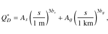
|
(9) |
where the first and the second term represent the strength and the gravity regime, respectively. We took values thought to be typical of low-temperature ice:
In the collisional simulation with ACE, we
refrain from testing various
possible material compositions of dust, for the following reasons.
First, each ACE run requires up
to a few weeks of computing time in parallel mode on
8-16 kernels.
Second, we would need to consistently modify both the optical constants
of the assumed material (that determine the strength of the radiation
pressure
force through ![]() )
and its mechanical properties that control
the collisional cascade. The latter would be problematic because of the
lack of
experimental data, for instance on QD*,
for non-icy materials.
Nevertheless, in Sect. 4, we will test the influence of
various materials
on the resulting termal emission of the EKB dust to get a rough idea of
the material dependence of the simulation results.
)
and its mechanical properties that control
the collisional cascade. The latter would be problematic because of the
lack of
experimental data, for instance on QD*,
for non-icy materials.
Nevertheless, in Sect. 4, we will test the influence of
various materials
on the resulting termal emission of the EKB dust to get a rough idea of
the material dependence of the simulation results.
In the ACE simulations, we used the
following
size-pericentric distance-eccentricity mesh.
The minimum grain radius was set to
![]() and the variable mass ratio in the adjacent bins between 4
(for largest TNOs)
and 2.1 (for dust sizes).
The pericenter distance grid covered 41 logarithmically-spaced
values
from 4 AU to 200 AU.
The eccentricity grid contained 50 linearly-spaced values
between -5.0 and 5.0 (eccentricities are negative in
the case of smallest
grains with
and the variable mass ratio in the adjacent bins between 4
(for largest TNOs)
and 2.1 (for dust sizes).
The pericenter distance grid covered 41 logarithmically-spaced
values
from 4 AU to 200 AU.
The eccentricity grid contained 50 linearly-spaced values
between -5.0 and 5.0 (eccentricities are negative in
the case of smallest
grains with ![]() ,
whose orbits are anomalous hyperbolas, open
outward from the star).
The distance grid used by ACE to output
distance-dependent
quantities such as the size distribution was 100 values
between 4 AU and 400 AU.
,
whose orbits are anomalous hyperbolas, open
outward from the star).
The distance grid used by ACE to output
distance-dependent
quantities such as the size distribution was 100 values
between 4 AU and 400 AU.
In many previous studies, the initial radial and size distributions of dust parent bodies - planetesimals - were taken in the form of power laws, with normalization factors and indices being parameters of the simulations. In this paper, we use a different approach. To take advantage of our knowledge of the (largest) parent bodies, TNOs, we directly filled the (m,q,e)-bins at the beginning of each simulation with the objects of the ``true'' Kuiper belt. For comparison, we also made a run, where we populated the bins with known TNOs only (without debiasing).
As already described, our ``true'' distribution contains only
big objects
with radii greater than ![]()
![]() ,
whereas in reality small objects at all sizes down to dust must be
present, too.
If we started a simulation without smaller objects, the collisional
cascade would take many gigayears to produce a noteworthy amount of
dust and to reach collisional
equilibrium.
Accordingly, we have extrapolated the contents of the filled bins
towards smaller
sizes with a slope of
q=3.03 for objects between
,
whereas in reality small objects at all sizes down to dust must be
present, too.
If we started a simulation without smaller objects, the collisional
cascade would take many gigayears to produce a noteworthy amount of
dust and to reach collisional
equilibrium.
Accordingly, we have extrapolated the contents of the filled bins
towards smaller
sizes with a slope of
q=3.03 for objects between
![]() (in the gravity regime)
and q=3.66 for objects smaller than
(in the gravity regime)
and q=3.66 for objects smaller than
![]() (in the strength regime),
following O'Brien
& Greenberg (2003). Note that the adopted slope in
the gravity regime is roughly consistent
with Fig. 8.
The break at radii of several tens of kilometers
reported by Bernstein
et al. (2004) and Fraser
(2009)
was not included.
In the course of the collisional evolution,
this artificial distribution corrects itself until it
comes to a collisional quasi-steady state.
The latter is assumed to have been reached, when the size distribution
no longer changes its shape and
just gradually moves down as a whole as a result of collisional
depletion
of parent bodies (Löhne
et al. 2008).
We find that after
(in the strength regime),
following O'Brien
& Greenberg (2003). Note that the adopted slope in
the gravity regime is roughly consistent
with Fig. 8.
The break at radii of several tens of kilometers
reported by Bernstein
et al. (2004) and Fraser
(2009)
was not included.
In the course of the collisional evolution,
this artificial distribution corrects itself until it
comes to a collisional quasi-steady state.
The latter is assumed to have been reached, when the size distribution
no longer changes its shape and
just gradually moves down as a whole as a result of collisional
depletion
of parent bodies (Löhne
et al. 2008).
We find that after ![]()
![]() a collisional quasi-steady
state sets in for all solids in the strength
regime (i.e., smaller than
a collisional quasi-steady
state sets in for all solids in the strength
regime (i.e., smaller than ![]()
![]() ).
This particularly means that the system ``does not remember'' anymore
the assumed initial distribution in this size range.
).
This particularly means that the system ``does not remember'' anymore
the assumed initial distribution in this size range.
We stress that the extrapolation of the observable EKB toward
smaller sizes
described above should not be misinterpreted as an attempt to describe
the primordial size distribution of solids in the early EKB. The latter
is set by the mechanism
of the initial planetesimal accretion, which is as yet unknown. In the
standard scenarios of ``slow'' accretion (e.g. Kenyon & Bromley 2008)
a broad size distribution is expected. In contrast, ``rapid''
scenarios, such as
the ``primary accretion'' mechanism proposed by Cuzzi et al. (2007)
or ``graviturbulent'' formation triggered by transient zones of high
pressure (Johansen
et al. 2006) or by streaming instabilities
(Johansen et al.
2007) all imply that most of the mass of just-formed
planetesimals was contained in
![]() bodies.
Whatever mechanism was at work, and whatever size distribution the EKB
in the early solar system had, in this study we are only interested in
the
present-day EKB. Thus the purpose of the extrapolation described above
is
merely to choose the initial size distribution across the sizes that
would be as close to collisional equilibrium with the present-day EKB
as possible.
bodies.
Whatever mechanism was at work, and whatever size distribution the EKB
in the early solar system had, in this study we are only interested in
the
present-day EKB. Thus the purpose of the extrapolation described above
is
merely to choose the initial size distribution across the sizes that
would be as close to collisional equilibrium with the present-day EKB
as possible.
3.2 Size distribution of dust
![\begin{figure}
\par\includegraphics[width=8.5cm]{14208fig10.eps}
\end{figure}](/articles/aa/full_html/2010/12/aa14208-10/img190.png)
|
Figure 10: Size distribution of the Kuiper belt dust at different distances. The vertical axis gives the cross section density per size decade. Top: the debiased EKB, without P-R effect; middle: the debiased EKB, with P-R effect; bottom: known EKB objects only, with P-R effect. |
| Open with DEXTER | |
Figure 10
depicts the simulated size distribution of the EKB dust.
We present three cases:
for the debiased EKB without (top panel) and with P-R included
(middle), as well as for the known EKB objects with
P-R effect, for comparison (bottom).
To explain the gross features of the size distributions shown in
Fig. 10,
we introduce the ratio of radiation pressure to gravity,
usually denoted as ![]() (Burns et al. 1979).
If a small dust grain is released after a collision from a nearly
circular orbit,
its eccentricity is
(Burns et al. 1979).
If a small dust grain is released after a collision from a nearly
circular orbit,
its eccentricity is
![]() .
This implies higher eccentricities for smaller grain sizes.
The orbits of sufficiently small grains with
.
This implies higher eccentricities for smaller grain sizes.
The orbits of sufficiently small grains with ![]() exceeding
exceeding ![]() 0.5
are unbound. Accordingly, the grain radius that corresponds
to
0.5
are unbound. Accordingly, the grain radius that corresponds
to ![]() is commonly referred to as blowout limit.
The blowout size for the assumed ideal material in the solar system is
is commonly referred to as blowout limit.
The blowout size for the assumed ideal material in the solar system is
![]() .
Typically, the amount of blowout grains instantaneously present in the
steady-state system is much less than the amount of slightly larger
grains in loosely bound orbits around the star.
This is because the dust production of the grains of adjacent sizes is
comparable, but the lifetime of bound grains (due to collisions) is
much
longer than the lifetime of blowout grains (disk-crossing timescale).
This explains a drop in the size distribution around the blowout size
which is seen in all three panels of Fig. 10.
.
Typically, the amount of blowout grains instantaneously present in the
steady-state system is much less than the amount of slightly larger
grains in loosely bound orbits around the star.
This is because the dust production of the grains of adjacent sizes is
comparable, but the lifetime of bound grains (due to collisions) is
much
longer than the lifetime of blowout grains (disk-crossing timescale).
This explains a drop in the size distribution around the blowout size
which is seen in all three panels of Fig. 10.
Another generic feature of the size distribution is that it
becomes narrower
at larger distances from the Sun. Were the parent bodies all confined
to a narrow radial belt, the distribution far outside would appear as a
narrow peak composed only of small, high-![]() ,
barely bound grains sent by radiation pressure into eccentric orbits
with large apocentric distances.
However, in the case of the EKB this
effect is somewhat washed out, since the radial distribution of parent
bodies
themselves (mostly, of scattered objects) is extended radially, as
discussed in Sect. 3.3. As a result, the size distribution
even at relatively
large distances (e.g.
,
barely bound grains sent by radiation pressure into eccentric orbits
with large apocentric distances.
However, in the case of the EKB this
effect is somewhat washed out, since the radial distribution of parent
bodies
themselves (mostly, of scattered objects) is extended radially, as
discussed in Sect. 3.3. As a result, the size distribution
even at relatively
large distances (e.g. ![]() )
is a superposition of such a narrow distribution
and a background broad distribution of particles produced at those
distances directly.
Only at largest distances, at which hardly any parent bodies are
present
(see
)
is a superposition of such a narrow distribution
and a background broad distribution of particles produced at those
distances directly.
Only at largest distances, at which hardly any parent bodies are
present
(see ![]() curve), the size distribution transforms to a predicted narrow
peak adjacent to the blowout size.
curve), the size distribution transforms to a predicted narrow
peak adjacent to the blowout size.
A direct comparison of our two simulations for the debiased
EKB, without and
with P-R effect, reveals some differences.
One obvious - and expected - difference is the one between the
![]() curves.
At this distance (and all the others inside the main belt) parent
bodies
are nearly absent; there are only some scattered TNOs,
see Fig. 1.
Accordingly, without P-R nearly no dust is present there. However, a
substantial
amount of small particles is present there in the P-R case, because
these are transported
there by the P-R drag.
curves.
At this distance (and all the others inside the main belt) parent
bodies
are nearly absent; there are only some scattered TNOs,
see Fig. 1.
Accordingly, without P-R nearly no dust is present there. However, a
substantial
amount of small particles is present there in the P-R case, because
these are transported
there by the P-R drag.
Outside ![]()
![]() ,
the size distributions without and with P-R
show more similarities than dissimilarities.
In particular, the maximum of the cross section
at
,
the size distributions without and with P-R
show more similarities than dissimilarities.
In particular, the maximum of the cross section
at ![]() is nearly the same.
At sizes
is nearly the same.
At sizes ![]() ,
the curves roughly follow a classical Dohnanyi's law
(cross section per size decade
,
the curves roughly follow a classical Dohnanyi's law
(cross section per size decade ![]() s-0.5).
The main difference is a dip of the size distribution in the region of
the classical
EKB that occurs at sizes of
s-0.5).
The main difference is a dip of the size distribution in the region of
the classical
EKB that occurs at sizes of
![]() in the P-R case, which is easy to explain.
The
in the P-R case, which is easy to explain.
The ![]() grains in the classical EKB region stay in nearly-circular orbits,
because their
grains in the classical EKB region stay in nearly-circular orbits,
because their ![]() ratio
is small and radiation pressure-induced eccentricities are low.
These grains are mainly destroyed in collisions with most abundant
smaller
grains, several
ratio
is small and radiation pressure-induced eccentricities are low.
These grains are mainly destroyed in collisions with most abundant
smaller
grains, several ![]() in size.
In the non-P-R case, the latter grains have their pericenters
within the classical belt. Thus the collisions are ``grazing'', the
collisional
velocities relatively low, and the collisional desctruction of
in size.
In the non-P-R case, the latter grains have their pericenters
within the classical belt. Thus the collisions are ``grazing'', the
collisional
velocities relatively low, and the collisional desctruction of
![]() grains
relatively inefficient.
When the P-R effect is switched on, this changes. The P-R transport
lowers the
pericenters of smaller projectiles, and in the classical belt, they
collide with
grains
relatively inefficient.
When the P-R effect is switched on, this changes. The P-R transport
lowers the
pericenters of smaller projectiles, and in the classical belt, they
collide with ![]() grains
at higher speeds, which enhances their destruction and produces the
dip.
Note that this effect is absent farther out from the Sun. At a
grains
at higher speeds, which enhances their destruction and produces the
dip.
Note that this effect is absent farther out from the Sun. At a
![]() distance,
for example, the collisions between smaller grains and
distance,
for example, the collisions between smaller grains and
![]() particles
always occur far from the pericenter. Thus the P-R effect has
little influence
on the collisional velocities, and the size distribution
in the non-P-R and P-R cases is similar.
particles
always occur far from the pericenter. Thus the P-R effect has
little influence
on the collisional velocities, and the size distribution
in the non-P-R and P-R cases is similar.
![\begin{figure}
\par\includegraphics[width=18cm]{14208fig11.eps}
\end{figure}](/articles/aa/full_html/2010/12/aa14208-10/img205.png)
|
Figure 11:
Radial distribution of parent bodies a), from
|
| Open with DEXTER | |
However, the dust distributions computed with P-R effect,
but for expected (i.e., debiased) EKB and known (not debiased) EKB,
which
are shown in middle and bottom panels of Fig. 10, exhibit a
striking difference.
The P-R effect has only a moderate influence on dust produced
by the
expected (debiased) EKB, but a strong one on dust generated solely by
known TNOs.
This needs to be explained.
The debiasing procedure makes the EKB more densely populated, and the
resulting
increase in the dustiness shortens collision timescales to make them
comparable with the P-R transport timescales.
The resulting optical depth of the dust disk is such that it lies
roughly between the collision-dominated and transport-dominated
regimes.
Without debiasing the parent body population, the dustiness of the disk
is by two orders of magnitude lower, and so is the optical depth of the
dust disk.
At that optical depth level, the EKB dust disk would be
transport-dominated
below ![]() (but still collision-dominated at larger sizes).
This is illustrated by the lowest panel in Fig. 10 that presents
the size distribution of dust that would be produced by known TNOs.
It is seen that the size distribution in such a transport-dominated
disk
differs from that in a collision-dominated one qualitatively.
From
(but still collision-dominated at larger sizes).
This is illustrated by the lowest panel in Fig. 10 that presents
the size distribution of dust that would be produced by known TNOs.
It is seen that the size distribution in such a transport-dominated
disk
differs from that in a collision-dominated one qualitatively.
From ![]() down to blowout limit, the size distribution flattens and turns over.
This is because the smaller the grains, the faster their inward
P-R drift.
This transport removes small grains from the collisionally active
region
and thus they are present in smaller amounts.
As a result, the maximum of the cross section density shifts towards
down to blowout limit, the size distribution flattens and turns over.
This is because the smaller the grains, the faster their inward
P-R drift.
This transport removes small grains from the collisionally active
region
and thus they are present in smaller amounts.
As a result, the maximum of the cross section density shifts towards
![]() particles.
particles.
3.3 Radial distribution of dust
Figure 11 presents the radial distribution of dust parent bodies and their dust, the latter simulated without and with P-R transport.
We start with a radial distribution of parent bodies, TNOs
themselves,
shown in Fig. 11a.
In contrast to Fig. 6,
we plot here the total cross section
of the TNOs instead of the mass they carry, because it is the cross
section
that characterizes the efficiency of TNOs as dust producers.
Besides, we use the distance from the Sun instead of the semimajor axis
as an argument.
Specifically, we plot the cross section in the
![]() -sized
TNOs,
but the
radial profile for larger objects look similar.
As expected, the distribution peaks in the region of the main belt (40-
-sized
TNOs,
but the
radial profile for larger objects look similar.
As expected, the distribution peaks in the region of the main belt (40-
![]() ),
where about 90% of the cross section comes from the classical
EKB
objects.
Outside
),
where about 90% of the cross section comes from the classical
EKB
objects.
Outside ![]()
![]() ,
the cross section is solely due to scattered objects.
The distribution of the latter is quite extended radially, it is nearly
flat
over a wide distance range from
,
the cross section is solely due to scattered objects.
The distribution of the latter is quite extended radially, it is nearly
flat
over a wide distance range from ![]()
![]() to more than
to more than
![]() .
.
We now move to a discussion of the radial distribution of
dust.
As noted above, smaller grains with higher ![]() ratios acquire
higher orbital eccentricities.
As the eccentricities of particles slightly above the blowout limit are
the highest,
their radial distribution is the broadest, whereas larger particles
stay more confined to their birth regions.
In Fig. 11b
this effect can be seen from how the curves gradually change from the
largest (
ratios acquire
higher orbital eccentricities.
As the eccentricities of particles slightly above the blowout limit are
the highest,
their radial distribution is the broadest, whereas larger particles
stay more confined to their birth regions.
In Fig. 11b
this effect can be seen from how the curves gradually change from the
largest (
![]() )
to the smallest bound grains (
)
to the smallest bound grains (
![]() ).
The former essentially follow the distribution of the parent bodies,
while the latter exhibit a more extended, flatter radial profile.
Finally, blowout grains (e.g., those with
).
The former essentially follow the distribution of the parent bodies,
while the latter exhibit a more extended, flatter radial profile.
Finally, blowout grains (e.g., those with
![]() have an
have an ![]() r-2distribution,
as expected for a set of hyperbolic orbits streaming outward from their
birth locations.
r-2distribution,
as expected for a set of hyperbolic orbits streaming outward from their
birth locations.
Including the P-R drag (Fig. 11c)
does little with largest grains, but modifies the profile of smaller
ones (![]()
![]() )
substantially.
The P-R transport inward steepens their profile.
Besides, small particles are now present in high amounts at smaller
distances, even where no parent bodies are present, in contrast to the
case
without P-R.
)
substantially.
The P-R transport inward steepens their profile.
Besides, small particles are now present in high amounts at smaller
distances, even where no parent bodies are present, in contrast to the
case
without P-R.
Figure 11d
is the same as
Fig. 11c,
but replotted in the same units as Fig. 1a in Moro-Martín &
Malhotra (2003).
Instead of treating the actual distribution of TNOs and their
collisional dust production, they assumed a simplified narrow birth
ring between
![]() and a constant dust production rate. Nonetheless, the general behavior
remains the same.
At
and a constant dust production rate. Nonetheless, the general behavior
remains the same.
At ![]() the number density begins to decrease rapidly
but we still have some parent bodies outside
the number density begins to decrease rapidly
but we still have some parent bodies outside
![]() which
produce dust, so that in our case the number density decreases more
gently.
which
produce dust, so that in our case the number density decreases more
gently.
3.4 Coupled size-radial distribution
Another view of the EKB dust can be achieved by plotting its combined radial and size distribution (Fig. 12). Besides presenting the same salient features as those discussed in Sects. 3.2 and 3.3, it emphasizes that radial and size distribution of dust in a debris disk are intrinsically coupled and cannot be treated independently of each other.
![\begin{figure}
\par\includegraphics[width=8.8cm]{14208fig12.eps}
\end{figure}](/articles/aa/full_html/2010/12/aa14208-10/img219.png)
|
Figure 12: The distribution of the cross section density of the EKB dust as a function of distance and grain sizes. The panels are as in Fig. 11. |
| Open with DEXTER | |
3.5 Optical depth
The radial profile of the normal geometrical optical depth is shown in
Fig. 13.
In the case of a disk dominated by the P-R effect, Strubbe & Chiang (2006)
calculated analytically the exponent of the optical depth profile
![]() to be
to be ![]() and
and ![]() in the outer and inner regions, respectively.
Without P-R effect, i.e. for a collision-dominated disk,
no dust is present interior to the parent bodies, and the outer slope
should be close to
in the outer and inner regions, respectively.
Without P-R effect, i.e. for a collision-dominated disk,
no dust is present interior to the parent bodies, and the outer slope
should be close to ![]() .
.
These slopes are in qualitative agreement with our simulations
(Fig. 13).
Taking the known EKB objects as dust sources and including the
P-R effect,
we find a nearly constant optical depth in the inner region and
a slope of ![]() in the outer disk, close enough
to predictions for a transport-dominated disk.
For the actual EKB dust disk and with the P-R effect taken
into account,
the result is intermediate between what is expected for
transport-dominated
and collision-dominated disks. This is seen from the inner profile
which is gently decreasing inward (cf. Fig. 1 of Wyatt 2005),
and from the outer slope of
in the outer disk, close enough
to predictions for a transport-dominated disk.
For the actual EKB dust disk and with the P-R effect taken
into account,
the result is intermediate between what is expected for
transport-dominated
and collision-dominated disks. This is seen from the inner profile
which is gently decreasing inward (cf. Fig. 1 of Wyatt 2005),
and from the outer slope of
![]() .
Finally, for the actual EKB dust disk, but with the P-R effect
switched off,
the profile is the one expected for collision-dominated disks.
The optical depth drops sharply inward from the main belt,
whereas in the outer region the slope is
.
Finally, for the actual EKB dust disk, but with the P-R effect
switched off,
the profile is the one expected for collision-dominated disks.
The optical depth drops sharply inward from the main belt,
whereas in the outer region the slope is
![]() .
That it is somewhat flatter than the analytic value
.
That it is somewhat flatter than the analytic value
![]() ,
traces back to a rather broad radial distribution of scattered TNOs
that make a considerable constribution to the overall dust profile.
,
traces back to a rather broad radial distribution of scattered TNOs
that make a considerable constribution to the overall dust profile.
![\begin{figure}
\par\includegraphics[width=8.8cm]{14208fig13.eps}
\end{figure}](/articles/aa/full_html/2010/12/aa14208-10/img227.png)
|
Figure 13: Normal optical depth of the Kuiper belt with and without P-R drag. Uranus and Neptune are shown for orientation, but were not included in the simulations. The optical depth for the known EKB is amplified by a factor of 100. |
| Open with DEXTER | |
For the debiased EKB and with P-R effect included, the normal optical
depth
peaks at ![]()
![]() at a level
of
at a level
of ![]()
![]() .
Besides the normal optical depth shown in Fig. 13,
we have calculated the in-plane optical depth.
Our result,
.
Besides the normal optical depth shown in Fig. 13,
we have calculated the in-plane optical depth.
Our result, ![]() outside
outside ![]() ,
is at least by a factor of 4 higher than the estimate by
Stern (1996) who found
,
is at least by a factor of 4 higher than the estimate by
Stern (1996) who found
![]() .
.
We finally note that the dust production rate for the expected
EKB in collisional equilibrium was calculated to ![]()
![]() and
is three times higher than the predicted rate of
and
is three times higher than the predicted rate of
![]() from Landgraf
et al. (2002)
on the base of in situ measurements of Pioneer 10
and 11.
from Landgraf
et al. (2002)
on the base of in situ measurements of Pioneer 10
and 11.
4 Spectral energy distribution
4.1 Parameters and materials
![\begin{figure}
\par\includegraphics[width=8.8cm]{14208fig14.eps}
\end{figure}](/articles/aa/full_html/2010/12/aa14208-10/img234.png)
|
Figure 14: Infrared excess of the Kuiper belt dust. a) the debiased EKB, without P-R effect; b) the debiased EKB, with P-R effect; c) known EKB objects only, with P-R effect (amplified by a factor of 100); d) the ratio of b) and c). Three curves in each panel a) to c) are based on the same ACE runs, but the thermal emission was calculated for three different materials: blackbody, astrosilicate, and ``dirty ice''. For comparison, observed SEDs of three other old Sun-like stars are shown with symbols. Photometric data for these stars are adapted from Tanner et al. (2009); Beichman et al. (2006); Chen et al. (2006); Lawler et al. (2009); Sheret et al. (2004); Moór et al. (2006); Greaves et al. (2004). |
| Open with DEXTER | |
The equilibrium temperatures of dust and their thermal emission were
calculated
in a standard way as described, for instance, in Krivov et al. (2008).
In these calculations we computed the solar photospheric spectrum with
the NextGen
grid of models (Hauschildt
et al. 1999), assuming
a G2V star of solar metallicity.
To get a rough idea of how the thermal flux is affected by (unknown)
chemical composition
of the dust, we tested three different cases: ideal material (blackbody
absorption and emission),
astrosilicate from Laor
& Draine (1993), and ``dirty ice''.
The latter is defined as a mixture consisting of
a water ice matrix (with constants from Warren
1984) contaminated with ![]() volume fraction of astronomical silicate (Laor
& Draine 1993).
This is similar to what, for instance, Yamamoto & Mukai (1998)
adopted
in their calculation of thermal emission of the EKB dust.
The refractive indices of the adopted ice-silicate mixture were
calculated by means of the Maxwell-Garnett theory.
This also explains our using
volume fraction of astronomical silicate (Laor
& Draine 1993).
This is similar to what, for instance, Yamamoto & Mukai (1998)
adopted
in their calculation of thermal emission of the EKB dust.
The refractive indices of the adopted ice-silicate mixture were
calculated by means of the Maxwell-Garnett theory.
This also explains our using ![]() silicate fraction:
silicate fraction:
![]() is an upper
limit for which the effective medium theory still provides accurate
results (Kolokolova
& Gustafson 2001). With a standard Mie algorithm, we
then computed
the absorption efficiency
is an upper
limit for which the effective medium theory still provides accurate
results (Kolokolova
& Gustafson 2001). With a standard Mie algorithm, we
then computed
the absorption efficiency ![]() as a function of size and wavelength.
as a function of size and wavelength.
4.2 Calculated flux
The resulting SEDs of the simulated EKB dust disk, as it would be seen
from a ![]() distance, are presented in Fig. 14.
Three different curves correspond to three materials described above.
Pure astrosilicate and the ice-silicate
mixture produce SEDs of similar shape and height, peaking at 50-
distance, are presented in Fig. 14.
Three different curves correspond to three materials described above.
Pure astrosilicate and the ice-silicate
mixture produce SEDs of similar shape and height, peaking at 50-
![]() with
a maximum flux at a level of several
with
a maximum flux at a level of several
![]() .
On the ``dirty ice'' curve, a typical water ice feature at
.
On the ``dirty ice'' curve, a typical water ice feature at ![]()
![]() is
seen.
This feature may have been detected in the disk of a young debris disk
star
HD 181327 (Chen
et al. 2008). The fact that the feature is located
near
the SED maximum may help finding water ice in other debris
disks by future
observations.
A comparison with the blackbody curve readily shows that it departs
from the two others
significantly. The maximum moves to
is
seen.
This feature may have been detected in the disk of a young debris disk
star
HD 181327 (Chen
et al. 2008). The fact that the feature is located
near
the SED maximum may help finding water ice in other debris
disks by future
observations.
A comparison with the blackbody curve readily shows that it departs
from the two others
significantly. The maximum moves to
![]() and the (sub)-mm flux
becomes by two orders of magnitude higher than in the two other cases.
This
result confirms earlier conclusion (see, e.g. Krivov et al. 2008;
Yamamoto
& Mukai 1998)
that the blackbody assumption is probably too crude and should not be
used
in modeling the thermal emission of debris disks.
and the (sub)-mm flux
becomes by two orders of magnitude higher than in the two other cases.
This
result confirms earlier conclusion (see, e.g. Krivov et al. 2008;
Yamamoto
& Mukai 1998)
that the blackbody assumption is probably too crude and should not be
used
in modeling the thermal emission of debris disks.
It is important to compare the calculated flux of the EKB dust
with measurements of other known debris disks. For this purpose, we
looked at photometric data for other Sun-like stars.
We have chosen three stars which possess well-known, bright excesses
(measured at many wavelengths from mid-IR to sub-mm), which have
spectral classes
not too far from solar G2, and which, like the Sun, are rather
old
(![]()
![]() ). These are
HD 48682 (
). These are
HD 48682 (![]() Aur,
G0V, at 17 pc distance, estimated age 0.6-
Aur,
G0V, at 17 pc distance, estimated age 0.6-
![]() ),
HD 10647 (q1 Eri, F8V, 17 pc,
),
HD 10647 (q1 Eri, F8V, 17 pc, ![]()
![]() ), and HD 10700 (
), and HD 10700 (![]() Cet,
G8V, 4 pc,
Cet,
G8V, 4 pc, ![]() ).
Their SEDs, normalized to
).
Their SEDs, normalized to
![]() ,
are overplottted in Fig. 14.
A comparison shows that their SEDs are similar in shape to the
simulated SED
of the EKB dust disk (for one of the two realistic materials, not
blackbody).
The maximum of the SEDs of the selected debris disk stars
lies at1
,
are overplottted in Fig. 14.
A comparison shows that their SEDs are similar in shape to the
simulated SED
of the EKB dust disk (for one of the two realistic materials, not
blackbody).
The maximum of the SEDs of the selected debris disk stars
lies at1 ![]()
![]() ,
i.e. at slightly longer wavelenghts than the maximum
of the EKB dust flux. This (moderate) difference in the peak
wavelengths of different SEDs may be caused by a choice of chemical
composition
of the disks, by different extentions of EKB and other debris disks, or
both.
,
i.e. at slightly longer wavelenghts than the maximum
of the EKB dust flux. This (moderate) difference in the peak
wavelengths of different SEDs may be caused by a choice of chemical
composition
of the disks, by different extentions of EKB and other debris disks, or
both.
The major difference between the EKB dust disk and extrasolar debris disks is, of course, the absolute level of the thermal emission fluxes. For dust maintained by the debiased EKB (panels a and b), the fluxes from far-IR to sub-mm are about one to two orders of magnitude lower that those of the reference stars. Obviously, this traces back to a much lower total mass of the EKB compared to that of the extrasolar Kuiper belts. The reasons for this difference are currently a matter of debate. For instance, Booth et al. (2009) argue that typical Kuiper belts around stars with observed debris disks may not have undergone a major depletion phase due to a ``Late Heavy Bombardment''. Currently, it is not known whether low-mass disks at the EKB level exist around other stars at all and, if they do, how common they are. This question can only be answered with future, more sensitive observations (for instance, with Herschel Space Observatory).
It is interesting to compare fluxes from the expected EKB dust
disk (Fig. 14b)
with those from the dust disk that would stem from the known TNOs,
without
debiasing. The corresponding SEDs, depicted in Fig. 14c, are completely
different. Apart from an expected reduction of the fluxes by almost two
orders of magnitude, two other effects are seen. One is that the
astrosilicate and ``dirty ice'' SEDs
come much closer to each other and to the blackbody curve. As a result,
their maxima
shift to longer wavelengths of ![]()
![]() .
Another effect is a disapperance of the water ice feature. Both effects
are easily explained by the major differences between
the size distribution of dust of the known and expected EKBs
(cf. middle and bottom panels in Fig. 10).
In the dust disk of the known EKB, the cross section, and thus the
thermal emission, are dominated by grains
.
Another effect is a disapperance of the water ice feature. Both effects
are easily explained by the major differences between
the size distribution of dust of the known and expected EKBs
(cf. middle and bottom panels in Fig. 10).
In the dust disk of the known EKB, the cross section, and thus the
thermal emission, are dominated by grains ![]()
![]() in
size.
Such big grains behave as black bodies and do not produce
any distinctive spectral features.
We also present the ratio of fluxes from the dust disks of the expected
and known
EKBs (Fig. 14d).
The aforementioned reduction of the fluxes is seen here even
better. The reduction factor,
in
size.
Such big grains behave as black bodies and do not produce
any distinctive spectral features.
We also present the ratio of fluxes from the dust disks of the expected
and known
EKBs (Fig. 14d).
The aforementioned reduction of the fluxes is seen here even
better. The reduction factor, ![]() 10 at wavelengths longward of
10 at wavelengths longward of ![]()
![]() ,
increases further at shorter wavelengths for ice-silicate and
especially astrosilicate grains.
Obviously, this is also a consequence of the change in the size
distribution
discussed above.
,
increases further at shorter wavelengths for ice-silicate and
especially astrosilicate grains.
Obviously, this is also a consequence of the change in the size
distribution
discussed above.
For three selected wavelengths of
![]() ,
,
![]() ,
and
,
and ![]() ,
the fluxes
calculated for the ``known'' and ``expected'' EKBs and for all three
materials
are also tabulated in Table 5.
Solar photosphereic fluxes are given for comparison.
These values are used below to assess the detectability of debris disks
with Herschel.
,
the fluxes
calculated for the ``known'' and ``expected'' EKBs and for all three
materials
are also tabulated in Table 5.
Solar photosphereic fluxes are given for comparison.
These values are used below to assess the detectability of debris disks
with Herschel.
4.3 Detectability of ``Kuiper belts''
Table 5:
Calculated flux of the known and expected Kuiper belt dust (including
the P-R-effect) and photospheric flux of the Sun at different
wavelengths from a ![]() distance.
distance.
We would like to estimate the level, down to which Herschel can detect faint debris disks, and then to compare that level with our EKB dust disk models.
The sensitivity limit of the PACS instrument of the Herschel
telescope
at ![]() in the scan-map mode for one hour exposure time
is
in the scan-map mode for one hour exposure time
is ![]() at a
at a ![]() uncertainty
level
uncertainty
level![]() ,
or
,
or ![]() at
at ![]() .
The background noise, of course, is highly variable from one star to
another.
For 133 target stars of the Open Time Key Program DUNES (DUst
around NEarby Stars), its average value at
.
The background noise, of course, is highly variable from one star to
another.
For 133 target stars of the Open Time Key Program DUNES (DUst
around NEarby Stars), its average value at
![]() is
is ![]() at
at ![]() .
Combining the instrument and the background noise leads to a limiting
flux
as low as
.
Combining the instrument and the background noise leads to a limiting
flux
as low as
![]() for one hour exposure time at a
for one hour exposure time at a ![]() uncertainty level.
Assuming that the
uncertainty level.
Assuming that the ![]() flux
is proportional to the total mass of a debris disk,
we can conclude that an extrasolar EKB analog with a mass
flux
is proportional to the total mass of a debris disk,
we can conclude that an extrasolar EKB analog with a mass
![]() will
be detectable from a distance of
will
be detectable from a distance of
![]() ,
assuming a ``dirty ice'' as a dust composition.
For silicate dust, the detectability limit would go down to
,
assuming a ``dirty ice'' as a dust composition.
For silicate dust, the detectability limit would go down to
![]() .
Additional uncertanties in the stellar photospheric flux
(
.
Additional uncertanties in the stellar photospheric flux
(![]()
![]() of
of ![]() ,
or
,
or ![]() )
increase these
values slightly to
)
increase these
values slightly to ![]()
![]() and
and ![]()
![]() ,
respectively.
,
respectively.
5 Summary and conclusions
In this paper, we attempted to construct a model of the solar system debris disk - Kuiper belt objects and their collisional debris. This was done in two major steps. First, we developed a new algorithm to remove the two largest selection effects from TNO observations, the inclination and the distance biases. Applying it to the database of 1260 known TNOs, we derived new estimates for the global parameters of the ``true'' Kuiper belt: its mass, orbital and size distribution. Second, treating the debiased populations of EKB objects as dust parent bodies, we employed our collisional code to simulate their dust disk. This has resulted in estimates of the size and radial distribution of dust in the transneptunian region, as well the optical depth of the Kuiper belt dust disk. We have also calculated the thermal emission of the Kuiper belt dust and compared the expected infrared fluxes with those of known debris disks around other Sun-like stars.
We draw the following conclusions:
- 1.
- The total mass of the EKB, including classical, resonant,
and scattered objects,
amounts to
 .
Without scattered objects, the mass reduces to
.
Without scattered objects, the mass reduces to
 .
These values are by about one order of magnitude higher than the
mass of the known TNOs.
.
These values are by about one order of magnitude higher than the
mass of the known TNOs.
- 2.
- The dust disks that would be produced by the known EKB and by the expected (i.e., debiased) one are shown to have distinctly different properties, as detailed below. Much of the difference in the size and radial distribution of dust of the two EKBs traces back to the increased total mass of TNOs after the debiasing.
- 3.
- The slope of the differential size distribution in the EKB
in the size range
 (absolute magnitudes 8.9>H>6)is found
to be
(absolute magnitudes 8.9>H>6)is found
to be  for the classical objects,
 for resonant ones,
and
for resonant ones,
and  for scattered TNOs.
This results in
for scattered TNOs.
This results in  for classical and all resonant objects together.
For the entire EKB (classical, resonant, and scattered TNOs),
we find
for classical and all resonant objects together.
For the entire EKB (classical, resonant, and scattered TNOs),
we find  .
.
- 4.
- If the debiased populations of TNOs are taken as dust
sources,
the dustiness of the disk is high enough to make collisional timescales
comparable to, or even shorter than, the radial transport timescales.
Thus the predicted Kuiper belt dust disk rather falls to the category
of
collision-dominated debris disks, to which all debris disks detected
so far around other stars belong, albeit it is already close to the
``boundary''
between collision-dominated and transport-dominated disks.
The simulated size distribution in the EKB dust disk shows a sharp
cutoff
at the radiation pressure blowout radius of

 .
The cross section
dominating radius is several times larger.
.
The cross section
dominating radius is several times larger.
- 5.
- For comparison, we have also considered the dust disk that
would be produced solely by known TNOs as parent bodies.
That disk would fall into the transport-dominated regime,
where the Poynting-Robertson drift timescales are shorter than the
collisional
timescales (at dust sizes).
The size distribution in such a disk is dramatically different from
the one expected in collision-dominated disks. While a cutoff at
remains,
the distribution between
and
several hundreds of
 is
nearly flat, and the cross section is now dominated by much larger
grains,
is
nearly flat, and the cross section is now dominated by much larger
grains,
 in
radius.
in
radius.
- 6.
- The radial distribution of the TNOs themselves
peaks in the region of the main belt (40-
 ),
where about 90% of the cross section comes from the classical
EKB
objects.
Outside
),
where about 90% of the cross section comes from the classical
EKB
objects.
Outside
 ,
the cross section is solely due to scattered objects.
The distribution of the latter is quite extended radially, being nearly
flat
over a wide distance range from
,
the cross section is solely due to scattered objects.
The distribution of the latter is quite extended radially, being nearly
flat
over a wide distance range from 
 to more than
 .
.
- 7.
- The radial distribution of dust grains with radii

 is
similar
to the distribution of the parent bodies described above.
At smaller sizes, the radial profile gets progressively broader with
decreasing
radius, which is a classical effect of radiation pressure.
is
similar
to the distribution of the parent bodies described above.
At smaller sizes, the radial profile gets progressively broader with
decreasing
radius, which is a classical effect of radiation pressure.
- 8.
- The maximum normal geometrical optical depth is reached at
the inner edge
of the classical belt,
 ,
and is estimated to be
,
and is estimated to be
 .
Outside that distance, it falls off as r-2.
This slope is roughly intermediate between the slope
predicted analytically for collision-dominated (r-1.5)
and transport-dominated (r-2.5)
disks.
An upper limit of the in-plane optical depth is set to
.
Outside that distance, it falls off as r-2.
This slope is roughly intermediate between the slope
predicted analytically for collision-dominated (r-1.5)
and transport-dominated (r-2.5)
disks.
An upper limit of the in-plane optical depth is set to
 outside
 .
.
- 9.
- For comparison, the normal optical depth of the
dust disk produced only by known TNOs would fall off
outside the classical EKB as
 ,
and the
in-plane optical depth would be by two orders of magnitude lower.
,
and the
in-plane optical depth would be by two orders of magnitude lower.
- 10.
- The estimated thermal emission flux from the EKB dust disk
that would be
observed from a
 distance strongly depends on the assumed dust composition.
For two ``realistic'' materials probed, astrosilicate and ice-silicate
mixture,
the SED would peak at 40-
distance strongly depends on the assumed dust composition.
For two ``realistic'' materials probed, astrosilicate and ice-silicate
mixture,
the SED would peak at 40-
 .
The maximum value is at a level of
several
.
The maximum value is at a level of
several  (at the solar photospheric flux at the same wavelengths
is several tens of
), which is about two orders
of magnitude smaller than for the brightest known debris disks around
other solar-type stars,
normalized to the same distance.
For a non-debiased EKB, the fluxes would be another two orders of
magnitude
lower.
(at the solar photospheric flux at the same wavelengths
is several tens of
), which is about two orders
of magnitude smaller than for the brightest known debris disks around
other solar-type stars,
normalized to the same distance.
For a non-debiased EKB, the fluxes would be another two orders of
magnitude
lower.
- 11.
- With the Herschel Space Observatory, it may be possible to
detect faint debris disks around other stars, which are nearly as faint
as the EKB dust disk.
For observations with the PACS instrument at
in a scan-map mode with one hour exposure, assuming an average
background noise, the minimum mass of a Kuiper belt analog detectable
at
 from
is estimated as
from
is estimated as
 .
.
6 Discussion
The main result of this paper is a set of new estimates of the parameters of the ``true'' (debiased) Kuiper belt and its debris dust. As all models, ours involves uncertainties. Here we discuss three major ones.
1. Parent bodies.
Although we believe that our debiasing algorithm is more accurate that
the ones used before, it is possible that the results over- or
underestimate,
for instance, the mass of the EKB by a factor of a few.
The main reason is an incomplete list of surveys used for debiasing.
In particular, observations that covered higher ecliptic latitudes,
omitted in Table 1,
could alter the results.
We have identified 90 objects in the MPC
(excluding Centaurs) that have been detected beyond ![]() ecliptic
latitude. Of these, 29 objects have been found beyond
ecliptic
latitude. Of these, 29 objects have been found beyond ![]() .
To check how non-including the surveys that covered higher latitudes
may affect the results, we have made additional tests. We have
re-run our code several times, each time artificially
changing
.
To check how non-including the surveys that covered higher latitudes
may affect the results, we have made additional tests. We have
re-run our code several times, each time artificially
changing
![]() in three randomly chosen
surveys of Table 1
to
in three randomly chosen
surveys of Table 1
to ![]() .
This changed the detection probability of single objects typically by
a few tenths of percent only. The change in the inferred total EKB mass
turned out to be larger, but still minor, 4%.
.
This changed the detection probability of single objects typically by
a few tenths of percent only. The change in the inferred total EKB mass
turned out to be larger, but still minor, 4%.
Another difficulty is related to the scattered objects
with their large eccentricities and inclinations.
Their average detection probability is very low, the resulting ``mass
amplification factor''
very high (![]() 25),
so that the estimated masses of objects can
considerably differ from the ``true'' ones.
25),
so that the estimated masses of objects can
considerably differ from the ``true'' ones.
The same applies to the treatment of the smallest objects
discovered so far,
a few kilometers is radius. If, for instance, the break
the size distribution at
![]() inferred by
Bernstein et al.
(2004) and Fraser (2009)
were included, this would reduce the overall amount of dust.
This would make the EKB dust disk ``more transport-dominated''
with all the consequences discussed above.
inferred by
Bernstein et al.
(2004) and Fraser (2009)
were included, this would reduce the overall amount of dust.
This would make the EKB dust disk ``more transport-dominated''
with all the consequences discussed above.
Being aware of such caveats, throughout the paper we always compare the known (not debiased) EKB with the expected (debiased) EKB. This applies to the EKB itself (Sect. 2), as well as to its dust (Sect. 3-4). We expect that the results obtained here for the known and debiased EKB would at least ``bracket'' the reality.
2. Material composition of solids. Realistic simulations would necessitate good knowledge of tens of parameters, such as the bulk density, porosity, shape, tensile strength, optical constants of solids in the EKB, and all this over an extremely broad range of sizes: from hundreds of kilometers (large TNOs) down to a fraction of a micrometer (tiniest dust grains). In this paper, we made a large set of simplifying assumptions, ignoring, in particular, any dependence of all these parameters on size, although such dependencies are expected. We only probed several different materials when calculating the thermal emission of dust in Sect. 4, and saw how sensitive the results are to the adopted absorption and emission efficiencies of grains. There are no reasons to think that variation of other parameters, for instance mechanical properties of different-sized solids in the collisional modeling, would alter the results to a lesser extent.
3. Modification of dust disk by Neptune.
As mentioned above, effects of giant planets on the dust distribution,
of which those by Neptune are the largest,
were not included in our simulations.
These effects are diverse and can alter the results substantially.
Neptune is expected to capture some grains stemming from non-resonant
KBOs and drifting inward by P-R effect
into mean-motion resonances
(e.g. Moro-Martín
& Malhotra 2002; Liou & Zook 1999).
Similarly, sufficiently large grains that derive from resonant TNOs
must stay locked in such resonances from the very beginning for
considerable time periods
(e.g. Wyatt
2006; Krivov et al. 2007).
This will cause an enhancement of dust density at resonance locations,
which was not modeled here.
Furthermore, the distribution of dust will exhibit azimuthal
clumps instead of being rotationally-symmetric, as was assumed in our
ACE simulations.
Next, many of the grains are in Neptune-crossing orbits, or reach such
orbits in the process of their inward drift. The probability of close
encounters
with Neptune is not negligible, especially for larger grains that
drift inward more slowly. Encounters would result in partial truncation
of the dust disk at the planet's orbit, i.e. in a drop of dust density
at ![]() .
Some of the grains will be ejected outward, which may affect
the collisional balance of the whole disk.
.
Some of the grains will be ejected outward, which may affect
the collisional balance of the whole disk.
For these reasons, the simulation results presented here should be treated as preliminary. We can hope that future, deeper, TNO surveys would lead to a better knowledge of the global parameters of the EKB acting as dust parent bodies. Further modeling work, perhaps with other methods, should help quantify the effects of Neptune on the dust distribution. Choosing the most adequate mechanical and optical properties of KBOs and their dust is probably the main difficulty. Eventually, many of the uncertainties could be minimized, and the models can be verified, if dust in the transneptunian region is detected in situ by dust detectors aboard space missions, such as New Horizons (Horányi et al. 2008). On any account, we consider this study as a reasonable starting point in developing more accurate models of the debris disk of our own solar system.
AcknowledgementsWe thank Mark Wyatt for stimulating discussions of several aspects of this work and useful suggestions, Sebastian Müller for assistance in thermal emission calculations presented in Sect. 4, and the anonymous reviewer for a useful referee report. This research was supported by the Deutsche Forschungsgemeinschaft (DFG), project number Kr 2164/8-1. A.K. and T.L. are grateful to the Isaac Newton Institute for Mathematical Sciences in Cambridge where part of this work was carried out in the framework of the program ``Dynamics of Discs and Planets''.
References
- Allen, R. L., Bernstein, G. M., & Malhotra, R. 2001, ApJ, 549, L241 [NASA ADS] [CrossRef] [MathSciNet] [Google Scholar]
- Barucci, M. A., Brown, M. E., Emery, J. P., & Merlin, F. 2008, in The Solar System Beyond Neptune, ed. M. A. Barucci, H. Boehnhardt, D. P. Cruikshank, & A. Morbidelli, 143 [Google Scholar]
- Beichman, C. A., Bryden, G., Stapelfeldt, K. R., et al. 2006, ApJ, 652, 1674 [NASA ADS] [CrossRef] [Google Scholar]
- Bernstein, G. M., Trilling, D. E., Allen, R. L., et al. 2004, AJ, 128, 1364 [NASA ADS] [CrossRef] [Google Scholar]
- Booth, M., Wyatt, M. C., Morbidelli, A., Moro-Martín, A., & Levison, H. F. 2009, MNRAS, 399, 385 [NASA ADS] [CrossRef] [Google Scholar]
- Brown, M. E. 2001, AJ, 121, 2804 [Google Scholar]
- Brucker, M. J., Grundy, W. M., Stansberry, J. A., et al. 2009, Icarus, 201, 284 [NASA ADS] [CrossRef] [Google Scholar]
- Burns, J. A., Lamy, P. L., & Soter, S. 1979, Icarus, 40, 1 [NASA ADS] [CrossRef] [Google Scholar]
- Chen, C. H., Sargent, B. A., Bohac, C., et al. 2006, ApJS, 166, 351 [NASA ADS] [CrossRef] [Google Scholar]
- Chen, C. H., Fitzgerald, M. P., & Smith, P. S. 2008, ApJ, 689, 539 [NASA ADS] [CrossRef] [Google Scholar]
- Chiang, E. I., & Brown, M. E. 1999, AJ, 118, 1411 [NASA ADS] [CrossRef] [Google Scholar]
- Cuzzi, J. N., Hogan, R. C., & Shariff, K. 2007, in Lunar and Planetary Inst. Technical Report, Lunar and Planetary Institute Science Conference Abstracts, 38, 1439 [Google Scholar]
- Delsanti, A., & Jewitt, D. 2006, The Solar System Beyond The Planets, ed. P. Blondel, & J. Mason (Springer), 267 [Google Scholar]
- Donnison, J. R. 2006, Planet. Space Sci., 54, 243 [NASA ADS] [CrossRef] [Google Scholar]
- Dumas, C., Merlin, F., Barucci, M. A., et al. 2007, A&A, 471, 331 [NASA ADS] [CrossRef] [EDP Sciences] [Google Scholar]
- Elliot, J. L., Kern, S. D., Clancy, K. B., et al. 2005, AJ, 129, 1117 [NASA ADS] [CrossRef] [Google Scholar]
- Fraser, W. C. 2009, ApJ, 706, 119 [NASA ADS] [CrossRef] [Google Scholar]
- Fraser, W. C., & Kavelaars, J. J. 2009, AJ, 137, 72 [NASA ADS] [CrossRef] [Google Scholar]
- Fraser, W. C., Kavelaars, J. J., Holman, M. J., et al. 2008, Icarus, 195, 827 [NASA ADS] [CrossRef] [Google Scholar]
- Fuentes, C. I., & Holman, M. J. 2008, AJ, 136, 83 [NASA ADS] [CrossRef] [Google Scholar]
- Fuentes, C. I., George, M. R., & Holman, M. J. 2009, ApJ, 696, 91 [NASA ADS] [CrossRef] [Google Scholar]
- Gladman, B., Kavelaars, J. J., Nicholson, P. D., Loredo, T. J., & Burns, J. A. 1998, AJ, 116, 2042 [NASA ADS] [CrossRef] [Google Scholar]
- Gladman, B., Kavelaars, J. J., Petit, J.-M., et al. 2001, AJ, 122, 1051 [NASA ADS] [CrossRef] [Google Scholar]
- Gomes, R., Levison, H. F., Tsiganis, K., & Morbidelli, A. 2005, Nature, 435, 466 [NASA ADS] [CrossRef] [PubMed] [Google Scholar]
- Greaves, J. S., Wyatt, M. C., Holland, W. S., & Dent, W. R. F. 2004, MNRAS, 351, L54 [NASA ADS] [CrossRef] [MathSciNet] [Google Scholar]
- Grün, E., Gustafson, B. A. S., Dermott, S., & Fechtig, H. 2001, Interplanetary Dust (Springer), 804 [Google Scholar]
- Gulbis, A., Elliot, J., Adams, E., et al. 2010, AJ, accepted [Google Scholar]
- Gurnett, D. A., Ansher, J. A., Kurth, W. S., & Granroth, L. J. 1997, Geophys. Res. Lett., 24, 3125 [Google Scholar]
- Hauschildt, P. H., Allard, F., & Baron, E. 1999, ApJ, 512, 377 [NASA ADS] [CrossRef] [Google Scholar]
- Horányi, M., Hoxie, V., James, D., et al. 2008, Space Sci. Rev., 140, 387 [NASA ADS] [CrossRef] [Google Scholar]
- Irwin, M., Tremaine, S., & Zytkow, A. N. 1995, AJ, 110, 3082 [NASA ADS] [CrossRef] [Google Scholar]
- Jewitt, D., Luu, J., & Marsden, B. G. 1992, IAU Circ., 5611, 1 [NASA ADS] [Google Scholar]
- Jewitt, D., Luu, J., & Chen, J. 1996, AJ, 112, 1225 [NASA ADS] [CrossRef] [Google Scholar]
- Jewitt, D., Luu, J., & Trujillo, C. 1998, AJ, 115, 2125 [NASA ADS] [CrossRef] [Google Scholar]
- Jewitt, D., Moro-Martìn, A., & Lacerda, P. 2009, The Kuiper Belt and Other Debris Disks, ed. H. A. Thronson, M. Stiavelli, & A. Tielens, 53 [Google Scholar]
- Jewitt, D. C., & Luu, J. X. 1995, AJ, 109, 1867 [NASA ADS] [CrossRef] [Google Scholar]
- Johansen, A., Klahr, H., & Henning, T. 2006, ApJ, 636, 1121 [NASA ADS] [CrossRef] [Google Scholar]
- Johansen, A., Oishi, J. S., Low, M.-M. M., et al. 2007, Nature, 448, 1022 [Google Scholar]
- Kavelaars, J. J., Jones, R. L., Gladman, B. J., et al. 2009, AJ, 137, 4917 [NASA ADS] [CrossRef] [Google Scholar]
- Kenyon, S. J., & Bromley, B. C. 2008, Astrophys. J. Suppl., 179, 451 [NASA ADS] [CrossRef] [Google Scholar]
- Kolokolova, L., & Gustafson, B. A. S. 2001, J. Quant. Spec. Radiat. Trans., 70, 611 [Google Scholar]
- Krivov, A. V. 2010, RA&A, 10, 383 [Google Scholar]
- Krivov, A. V., Mann, I., & Krivova, N. A. 2000, A&A, 362, 1127 [NASA ADS] [Google Scholar]
- Krivov, A. V., Löhne, T., & Sremcevic, M. 2006, A&A, 455, 509 [NASA ADS] [CrossRef] [EDP Sciences] [Google Scholar]
- Krivov, A. V., Müller, S., Löhne, T., & Mutschke, H. 2008, ApJ, 687, 608 [NASA ADS] [CrossRef] [Google Scholar]
- Krivov, A. V., Queck, M., Löhne, T., & Sremcevic, M. 2007, A&A, 462, 199 [NASA ADS] [CrossRef] [EDP Sciences] [Google Scholar]
- Krivov, A. V., Sremcevic, M., & Spahn, F. 2005, Icarus, 174, 105 [NASA ADS] [CrossRef] [Google Scholar]
- Kuchner, M. J., & Stark, C. C. 2010, AJ, submitted [Google Scholar]
- Lacerda, P. 2009, in SPICA joint European/Japanese Workshop, held 6-8 July, at Oxford, United Kingdom, ed. A. M. Heras, B. M. Swinyard, K. G. Isaak, & J. R. Goicoechea, EDP Sciences, 02004, 2004 [Google Scholar]
- Lamy, P. L., Toth, I., Fernandez, Y. R., & Weaver, H. A. 2004, The sizes, shapes, albedos, and colors of cometary nuclei, ed. M. C. Festou, H. U. Keller, & H. A. Weaver, 223 [Google Scholar]
- Landgraf, M., Liou, J.-C., Zook, H. A., & Grün, E. 2002, AJ, 123, 2857 [NASA ADS] [CrossRef] [Google Scholar]
- Laor, A., & Draine, B. T. 1993, ApJ, 402, 441 [NASA ADS] [CrossRef] [Google Scholar]
- Larsen, J. A., Roe, E. S., Albert, C. E., et al. 2007, AJ, 133, 1247 [NASA ADS] [CrossRef] [Google Scholar]
- Lawler, S. M., Beichman, C. A., Bryden, G., et al. 2009, ApJ, 705, 89 [NASA ADS] [CrossRef] [Google Scholar]
- Liou, J.-C., & Zook, H. A. 1999, AJ, 118, 580 [NASA ADS] [CrossRef] [Google Scholar]
- Lissauer, J. J. 1987, Icarus, 69, 249 [NASA ADS] [CrossRef] [Google Scholar]
- Löhne, T., Krivov, A. V., & Rodmann, J. 2008, ApJ, 673, 1123 [NASA ADS] [CrossRef] [Google Scholar]
- Luu, J. X., & Jewitt, D. C. 1998, ApJ, 502, L91 [NASA ADS] [CrossRef] [Google Scholar]
- Luu, J. X., & Jewitt, D. C. 2002, ARA&A, 40, 63 [NASA ADS] [CrossRef] [MathSciNet] [Google Scholar]
- Moór, A., Ábrahám, P., Derekas, A., et al. 2006, ApJ, 644, 525 [NASA ADS] [CrossRef] [Google Scholar]
- Moro-Martín, A., & Malhotra, R. 2002, AJ, 124, 2305 [NASA ADS] [CrossRef] [Google Scholar]
- Moro-Martín, A., & Malhotra, R. 2003, AJ, 125, 2255 [NASA ADS] [CrossRef] [Google Scholar]
- Müller, S., Löhne, T., & Krivov, A. V. 2010, ApJ, 708, 1728 [NASA ADS] [CrossRef] [Google Scholar]
- Murray, C. D., & Dermott, S. F. 2000, Solar System Dynamics, ed. C. D. Murray, & S. F. Dermott (Cambridge, UK: Cambridge University Press) [Google Scholar]
- Noll, K. S., Stephens, D. C., Grundy, W. M., Osip, D. J., & Griffin, I. 2004, AJ, 128, 2547 [NASA ADS] [CrossRef] [Google Scholar]
- O'Brien, D. P., & Greenberg, R. 2003, Icarus, 164, 334 [CrossRef] [Google Scholar]
- Petit, J.-M., Holman, M. J., Gladman, B. J., et al. 2006, MNRAS, 365, 429 [NASA ADS] [CrossRef] [Google Scholar]
- Pinilla-Alonso, N., Brunetto, R., Licandro, J., et al. 2009, A&A, 496, 547 [NASA ADS] [CrossRef] [EDP Sciences] [Google Scholar]
- Quinn, T., Tremaine, S., & Duncan, M. 1990, ApJ, 355, 667 [NASA ADS] [CrossRef] [Google Scholar]
- Safronov, V. S. 1969, Evolution of the Protoplanetary Cloud and Formation of the Earth and Planets (Nauka, Moscow, in Russian; English translation: NASA TTF-677, 1972) [Google Scholar]
- Sheret, I., Dent, W. R. F., & Wyatt, M. C. 2004, MNRAS, 348, 1282 [NASA ADS] [CrossRef] [Google Scholar]
- Stansberry, J., Grundy, W., Brown, M., et al. 2008, Physical Properties of Kuiper Belt and Centaur Objects: Constraints from the Spitzer Space Telescope (The Solar System Beyond Neptune) [Google Scholar]
- Stern, S. A. 1995, AJ, 110, 856 [NASA ADS] [CrossRef] [Google Scholar]
- Stern, S. A. 1996, A&A, 310, 999 [NASA ADS] [Google Scholar]
- Strubbe, L. E., & Chiang, E. I. 2006, ApJ, 648, 652 [NASA ADS] [CrossRef] [Google Scholar]
- Tanner, A., Beichman, C., Bryden, G., Lisse, C., & Lawler, S. 2009, ApJ, 704, 109 [NASA ADS] [CrossRef] [Google Scholar]
- Thébault, P., & Augereau, J. 2007, A&A, 472, 169 [NASA ADS] [CrossRef] [EDP Sciences] [Google Scholar]
- Thébault, P., Augereau, J. C., & Beust, H. 2003, A&A, 408, 775 [NASA ADS] [CrossRef] [EDP Sciences] [Google Scholar]
- Trujillo, C. A., & Brown, M. E. 2003, Earth Moon and Planets, 92, 99 [Google Scholar]
- Trujillo, C. A., Jewitt, D. C., & Luu, J. X. 2000, ApJ, 529, L103 [NASA ADS] [CrossRef] [PubMed] [Google Scholar]
- Trujillo, C. A., Jewitt, D. C., & Luu, J. X. 2001a, AJ, 122, 457 [NASA ADS] [CrossRef] [Google Scholar]
- Trujillo, C. A., Luu, J. X., Bosh, A. S., & Elliot, J. L. 2001b, AJ, 122, 2740 [NASA ADS] [CrossRef] [Google Scholar]
- Warren, S. G. 1984, App. Opt., 23, 1206 [Google Scholar]
- Wetherill, G. W. 1980, ARA&A, 18, 77 [NASA ADS] [CrossRef] [Google Scholar]
- Wyatt, M. C. 2005, A&A, 433, 1007 [NASA ADS] [CrossRef] [EDP Sciences] [Google Scholar]
- Wyatt, M. C. 2006, ApJ, 639, 1153 [NASA ADS] [CrossRef] [Google Scholar]
- Wyatt, M. C. 2008, ARA&A, 46, 339 [NASA ADS] [CrossRef] [Google Scholar]
- Wyatt, M. C., Smith, R., Su, K. Y. L., et al. 2007, ApJ, 663, 365 [NASA ADS] [CrossRef] [Google Scholar]
- Yamamoto, S., & Mukai, T. 1998, Earth, Planets and Space, 50, 531 [Google Scholar]
Footnotes
- ...
database
![[*]](/icons/foot_motif.png)
- http://www.cfa.harvard.edu/iau/lists/TNOs.html (Last accessed 12 October 2009).
- ...
level
- http://herschel.esac.esa.int/Docs/PACS/html/ch03s05.html#sec-photo-sensitivity
All Tables
Table 1: A list of campaigns where TNOs were found.
Table 2: Masses and numbers of objects in the Kuiper belt.
Table 3:
Masses of objects in the Kuiper belt, as a function of the assumed
relative accuracy ![]() ,
with which orbital elements of TNOs were deduced from observations.
,
with which orbital elements of TNOs were deduced from observations.
Table 4: Size distribution index of the Kuiper belt populations.
Table 5:
Calculated flux of the known and expected Kuiper belt dust (including
the P-R-effect) and photospheric flux of the Sun at different
wavelengths from a ![]() distance.
distance.
All Figures
|
|
Figure 1:
Known TNOs in the a-e plane
(top) and a-i plane (bottom).
Different groups are shown with different symbols:
865 classical objects with dots, 235 resonant TNOs
with pluses, and the remaining 160 scattered objects with
crosses. Solid lines separate classical and scattered objects in our
classification. One object with
|
| Open with DEXTER | |
| In the text | |
|
|
Figure 2:
Observable arc(s) of a TNO orbit that satisfy the distance and the
inclination restrictions. Smaller points denoted with E1
and E2 are intersection
points of the orbit with the sphere
|
| Open with DEXTER | |
| In the text | |
|
|
Figure 3:
The detection probability of all known TNOs (as function of their
orbital inclinations) in a fiducial survey with a full coverage of a
belt on the sky within
|
| Open with DEXTER | |
| In the text | |
|
|
Figure 4: The final detection probability of the known TNOs, calculated with Eq. (4). Included are all surveys from Table 1. |
| Open with DEXTER | |
| In the text | |
|
|
Figure 5:
Distribution of classical (top row), resonant (middle
row), and scattered objects (bottom row),
in terms of numbers of objects. Left column:
semimajor axes, middle: eccentricities,
right: inclinations. Black and grey bars in each panel
represent the expected (unbiased) and observed populations,
respectively. The numbers of the observed TNOs are magnified
by 20 (classical and resonant objects) and 50
(scattered objects) for better visibility. Numbers are given
in 1000 for intervals with a width of
|
| Open with DEXTER | |
| In the text | |
|
|
Figure 6: Same as Fig. 5, but in terms of mass contained in TNOs. |
| Open with DEXTER | |
| In the text | |
|
|
Figure 7:
Absolute magnitude - radius relation for objects with known albedo. The
biggest objects are labeled with their names. The thick solid line is a
fit to this relation, Eqs. (7)-(8). Thin lines
correspond to equal albedos of
|
| Open with DEXTER | |
| In the text | |
|
|
Figure 8:
Cumulative numbers of the expected and known Kuiper belt objects with a
|
| Open with DEXTER | |
| In the text | |
|
|
Figure 9: Phase-space distribution (in e,q-plane) of dust maintained by the expected EKB. Top: without P-R effect, bottom: with P-R effect. Pericenter distances are in AU. Eccentricities e<-1 correspond to anomalous hyperbolas open outward from the Sun. Grayscale gives the total cross section of dust, integrated over all sizes (in arbitrary units). |
| Open with DEXTER | |
| In the text | |
|
|
Figure 10: Size distribution of the Kuiper belt dust at different distances. The vertical axis gives the cross section density per size decade. Top: the debiased EKB, without P-R effect; middle: the debiased EKB, with P-R effect; bottom: known EKB objects only, with P-R effect. |
| Open with DEXTER | |
| In the text | |
|
|
Figure 11:
Radial distribution of parent bodies a), from
|
| Open with DEXTER | |
| In the text | |
|
|
Figure 12: The distribution of the cross section density of the EKB dust as a function of distance and grain sizes. The panels are as in Fig. 11. |
| Open with DEXTER | |
| In the text | |
|
|
Figure 13: Normal optical depth of the Kuiper belt with and without P-R drag. Uranus and Neptune are shown for orientation, but were not included in the simulations. The optical depth for the known EKB is amplified by a factor of 100. |
| Open with DEXTER | |
| In the text | |
|
|
Figure 14: Infrared excess of the Kuiper belt dust. a) the debiased EKB, without P-R effect; b) the debiased EKB, with P-R effect; c) known EKB objects only, with P-R effect (amplified by a factor of 100); d) the ratio of b) and c). Three curves in each panel a) to c) are based on the same ACE runs, but the thermal emission was calculated for three different materials: blackbody, astrosilicate, and ``dirty ice''. For comparison, observed SEDs of three other old Sun-like stars are shown with symbols. Photometric data for these stars are adapted from Tanner et al. (2009); Beichman et al. (2006); Chen et al. (2006); Lawler et al. (2009); Sheret et al. (2004); Moór et al. (2006); Greaves et al. (2004). |
| Open with DEXTER | |
| In the text | |
Copyright ESO 2010
Current usage metrics show cumulative count of Article Views (full-text article views including HTML views, PDF and ePub downloads, according to the available data) and Abstracts Views on Vision4Press platform.
Data correspond to usage on the plateform after 2015. The current usage metrics is available 48-96 hours after online publication and is updated daily on week days.
Initial download of the metrics may take a while.