| Issue |
A&A
Volume 520, September-October 2010
|
|
|---|---|---|
| Article Number | A115 | |
| Number of page(s) | 10 | |
| Section | Astronomical instrumentation | |
| DOI | https://doi.org/10.1051/0004-6361/200913441 | |
| Published online | 13 October 2010 | |
Two-dimensional solar spectropolarimetry with the KIS/IAA Visible Imaging Polarimeter
C. Beck1,2 - L. R. Bellot Rubio3 - T. J. Kentischer4 - A. Tritschler5 - J. C. del Toro Iniesta3
1 - Instituto de Astrofísica de Canarias (IAC), C/Vía Láctea S/N,
38205 La Laguna, Tenerife, Spain
2 - Departamento de Astrofísica, Universidad de La Laguna, 38205 La Laguna, Tenerife, Spain
3 -
Instituto de Astrofísica de Andalucía (CSIC), Apdo. de Correos 3004,
18080 Granada, Spain
4 -
Kiepenheuer-Institut für Sonnenphysik, Schöneckstr. 6, 79104
Freiburg, Germany
5 -
National Solar Observatory/Sacramento Peak![]() , PO Box 62, Sunspot, NM 88349, USA
, PO Box 62, Sunspot, NM 88349, USA
Received 9 October 2009 / Accepted 28 June 2010
Abstract
Context. Spectropolarimetry at high spatial and spectral
resolution is a basic tool to characterize the magnetic properties of
the solar atmosphere.
Aims. We introduce the KIS/IAA Visible Imaging Polarimeter
(VIP), a new post-focus instrument that upgrades the TESOS spectrometer
at the German Vacuum Tower Telescope (VTT) into a full vector
polarimeter. VIP is a collaboration between the Kiepenheuer Institut
für Sonnenphysik (KIS) and the Instituto de Astrofísica de Andalucía
(IAA-CSIC).
Methods. We describe the optical setup of VIP, the data
acquisition procedure, and the calibration of the spectropolarimetric
measurements. We show examples of data taken between 2005 and 2008 to
illustrate the potential of the instrument.
Results. VIP is capable of measuring the four Stokes profiles of
spectral lines in the range from 420 to 700 nm with a spatial
resolution better than 0
![]() 5. Lines can be sampled at 40 wavelength positions in 60 s, achieving a noise level of about
5. Lines can be sampled at 40 wavelength positions in 60 s, achieving a noise level of about
![]() with exposure times of 300 ms and pixel sizes of
with exposure times of 300 ms and pixel sizes of
![]() (
(![]() binning).
The polarization modulation is stable over periods of a few days,
ensuring high polarimetric accuracy. The excellent spectral resolution
of TESOS allows the use of sophisticated data analysis techniques such
as Stokes inversions. One of the first scientific results of VIP
presented here is that the ribbon-like magnetic structures of the
network are associated with a distinct pattern of net circular
polarization away from disk center.
binning).
The polarization modulation is stable over periods of a few days,
ensuring high polarimetric accuracy. The excellent spectral resolution
of TESOS allows the use of sophisticated data analysis techniques such
as Stokes inversions. One of the first scientific results of VIP
presented here is that the ribbon-like magnetic structures of the
network are associated with a distinct pattern of net circular
polarization away from disk center.
Conclusions. VIP performs spectropolarimetric measurements of
solar magnetic fields at a spatial resolution that is only slightly
worse than that of the Hinode spectropolarimeter, while
providing a 2D field field of view and the possibility to observe up to
four spectral regions sequentially with high cadence. VIP can be used
as a stand-alone instrument or in combination with other
spectropolarimeters and imaging systems of the VTT for extended
wavelength coverage.
Key words: instrumentation: polarimeters - Sun: photosphere - magnetic fields
1 Introduction
Measurements of the solar magnetic field and the determination of the thermal and kinematic properties of the magnetized atmosphere is a persistently challenging goal. The combination of high spectral and angular resolution is of vital importance for an accurate characterization of the atmospheric parameters in different structures, from the tiny magnetic elements of the quiet Sun to the largest sunspots. However, only a few ground-based instruments are capable of high-precision polarimetric observations with an angular resolution ofTwo different concepts have been followed to obtain measurements of the full Stokes vector at high spectral resolution: imaging and grating (slit-based) spectropolarimeters. Modern imaging spectropolarimeters employ single (see, e.g., Mickey et al. 1996) or multiple Fabry-Pérot etalons (FPIs) for fast tuning and high transmission. Several FPI spectropolarimeters are operated at present: the Göttingen spectropolarimeter (GFPI, Bello González & Kneer 2008), the Interferometric BIdimensional Spectrometer (IBIS, Reardon & Cavallini 2008; Cavallini 2006), and the CRisp Imaging Spectro-Polarimeter (CRISP, Scharmer et al. 2008). These instruments differ mostly in how the FPIs are mounted (telecentric or collimated) and in the spectral resolution.
In the category of slit-based spectropolarimeters, we have the
Advanced Stokes Polarimeter (ASP, Skumanich et al. 1997)
which has been superseded by the the Diffraction-Limited
Spectro-Polarimeter (DLSP, Sankarasubramanian et al. 2003),
the multiline polarimetric mode of THEMIS
(MTR, Rayrole & Mein 1993; López Ariste et al. 2000), the
POlarimetric LIttrow Spectrograph (POLIS, Beck et al. 2005b),
the Spectro-Polarimeter for Infrared and Optical Regions
(SPINOR, Socas-Navarro et al. 2006), and the Facility InfraRed
Spectropolarimeter (FIRS, Jaeggli et al. 2008). DLSP and POLIS
work at a fixed wavelength in the visible (630 nm), while SPINOR
and FIRS allow to observe different spectral regions in the visible
and the infrared. The Tenerife Infrared Polarimeter
(TIP, Collados et al. 2007; Martínez Pillet et al. 1999) can observe any
part of the near-infrared spectrum from 1 to 2.2 ![]() m using the main
spectrograph of the German Vacuum Tower Telescope (VTT). It regularly
reaches the diffraction limit at these wavelengths (about 0
m using the main
spectrograph of the German Vacuum Tower Telescope (VTT). It regularly
reaches the diffraction limit at these wavelengths (about 0
![]() 6).
6).
All ground-based instruments suffer from wavefront distortions caused
by turbulence in the Earths' atmosphere. Adaptive optic systems
(AO, Scharmer et al. 2003; Rimmele 2004; von der Lühe et al. 2003) are
mandatory to improve the image quality, but the compensation is only
partial and sub-arcsec resolution is hard to reach. Whereas in
slit-based spectropolarimetry no further improvement can be achieved
beyond what is delivered by the AO system, two-dimensional
spectropolarimetric observations can benefit from post-facto image
reconstruction techniques like de-stretching, speckle deconvolution
(see, e.g., Bello González & Kneer 2008; Puschmann & Sailer 2006; Keller & von der Luehe 1992; Mikurda et al. 2006), and MOMFBD (van Noort et al. 2005). At present, the only
instrument capable of delivering continuous measurements at 0
![]() 3
resolution is the spectropolarimeter (SP) of the Hinode
satellite (Kosugi et al. 2007). The Imaging Magnetograph eXperiment
(IMaX, Álvarez-Herrero et al. 2006; Jochum et al. 2003; Martínez Pillet et al. 2004)
aboard the SUNRISE balloon (Gandorfer et al. 2006) recently
completed its first flight and took data of even higher
resolution thanks to its 1-m telescope.
3
resolution is the spectropolarimeter (SP) of the Hinode
satellite (Kosugi et al. 2007). The Imaging Magnetograph eXperiment
(IMaX, Álvarez-Herrero et al. 2006; Jochum et al. 2003; Martínez Pillet et al. 2004)
aboard the SUNRISE balloon (Gandorfer et al. 2006) recently
completed its first flight and took data of even higher
resolution thanks to its 1-m telescope.
However, accurate spectropolarimetry does not only depend on spatial
resolution, but also on the precision achieved in the determination of
the polarization state. This is typically quantified by the
root-mean-square (rms) noise of Stokes QUV at continuum wavelengths
or by the signal-to-noise ratio (SNR) in the intensity spectrum.
Slit spectropolarimeters have the advantage that the spectrum is
detected instantly. Hence, an increase in exposure time or the
accumulation of spectra do not compromise the spectral purity or
integrity of the data. With integration times of 20-30 s, the rms
noise can be reduced to a few 10-4 of the continuum intensity
(Khomenko et al. 2003; Beck & Rezaei 2009; Martínez González et al. 2008; Bommier & Molodij 2002).
For FPI-based instruments this is more difficult due to the
sequential wavelength scanning. To obtain the SNR of a typical
slit-spectrograph spectrum, a 2D instrument has to use a similar
integration time for every wavelength position, which usually
makes the line scan unacceptably long (>2 min). Hence, for all
2D-type spectropolarimeters a compromise has to be found between
SNR, spectral sampling, and angular resolution. A SNR comparable to
that of long-integrated (![]() 5 s) slit-spectra cannot be
obtained with any currently existing 2D instrument.
5 s) slit-spectra cannot be
obtained with any currently existing 2D instrument.
However, these instruments also have great advantages compared to slit
systems. First, they are flexible in wavelength range. Even if the
various spectral regions can be observed sequentially only, the
cadence may be sufficiently high to treat them as simultaneous,
depending on the scientific problem. For slit-based systems, a change
of the spectral region usually requires changes in the setup, or is even
impossible because of fixed gratings (DLSP, POLIS, Hinode/SP). Second, 2D instruments provide spatially coherent
observations with much faster cadence than is possible with slit
systems. In high-resolution mode, when small step sizes are involved
(e.g., 0
![]() 15 in the case of the Hinode/SP or the DLSP),
slit-spectrograph systems do not attain the cadence needed to
follow the solar evolution with sufficient spatial coverage. Fast
events, particularly in the solar chromosphere with time
scales of 30 s or less (Rutten & Uitenbroek 1991; Beck et al. 2008; Wedemeyer et al. 2004; Wöger et al. 2006; Carlsson & Stein 1997), can only be traced on very small
FOVs, whereas the spatial extent of the phenomenon may excess the scan
area easily.
15 in the case of the Hinode/SP or the DLSP),
slit-spectrograph systems do not attain the cadence needed to
follow the solar evolution with sufficient spatial coverage. Fast
events, particularly in the solar chromosphere with time
scales of 30 s or less (Rutten & Uitenbroek 1991; Beck et al. 2008; Wedemeyer et al. 2004; Wöger et al. 2006; Carlsson & Stein 1997), can only be traced on very small
FOVs, whereas the spatial extent of the phenomenon may excess the scan
area easily.
The Triple Etalon SOlar Spectrometer (TESOS, Kentischer et al. 1998; Tritschler et al. 2002) at the German VTT in Tenerife was a natural candidate for an upgrade into a vector polarimeter. TESOS features high spectral resolution and is the only triple-FPI system in operation to date. The unique spectroscopic capabilities of TESOS have been used to study the kinematic and thermal properties of several magnetic and non-magnetic structures (see, e.g., Bellot Rubio et al. 2006; Schmidt & Schlichenmaier 2000; Langhans et al. 2002; Tritschler et al. 2004; Schleicher et al. 2003; Mikurda et al. 2006; Schlichenmaier et al. 2004; Schlichenmaier & Schmidt 1999). However, although valuable for the analysis of photospheric velocity fields and temperatures, these observations do not provide information about the magnetic field.
Here we describe the KIS/IAA Visible Imaging Polarimeter (VIP), the polarization package that converts TESOS into a full vector spectropolarimeter. Section 2 gives an overview of the optical layout of TESOS in polarimetric mode, focusing on the modulation package and the detectors. The data acquisition and the calibration procedure are explained in Sects. 3 and 4, respectively. In Sect. 5, we present three examples of VIP observations to illustrate the capabilities of the instrument. Our conclusions are summarized in Sect. 6.
|
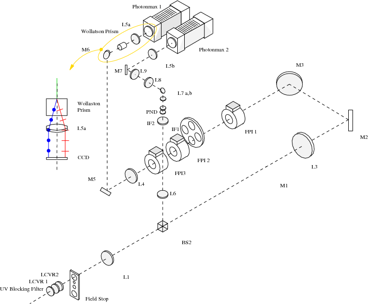
Figure 1:
Optical setup of TESOS in high resolution mode. The light
undergoes four |
| Open with DEXTER | |
2 Instrument description
TESOS is a Fabry-Pérot spectrometer in a telecentric configuration
(Kentischer et al. 1998; Tritschler et al. 2002). Figure 1 sketches the optical layout with its current components. The three etalons significantly reduce side-lobe
influence and permit the use of broad prefilters (![]() 1 nm FWHM)
with typical transmissions of 75%. In high resolution mode, the
spectral resolution of the instrument is of the order of 300 000
at 632.8 nm, comparable with classical slit spectrographs. Up to
four spectral lines can be observed sequentially thanks to the
motorized filter wheel (IF1 in Fig. 1). Combined with
the Kiepenheuer Adaptive Optics System (von der Lühe et al. 2003), TESOS
is able to achieve a spatial resolution of about 0
1 nm FWHM)
with typical transmissions of 75%. In high resolution mode, the
spectral resolution of the instrument is of the order of 300 000
at 632.8 nm, comparable with classical slit spectrographs. Up to
four spectral lines can be observed sequentially thanks to the
motorized filter wheel (IF1 in Fig. 1). Combined with
the Kiepenheuer Adaptive Optics System (von der Lühe et al. 2003), TESOS
is able to achieve a spatial resolution of about 0
![]() 5 on a regular
basis.
5 on a regular
basis.
Polarimetry was one of the science drivers of TESOS from the
beginning (see Kentischer et al. 1998). To minimize instrumental
polarization, the four folding mirrors inside TESOS were arranged in
such a way that two sagittal 45![]() reflections are followed by
two tangential 45
reflections are followed by
two tangential 45![]() reflections. This configuration does not
introduce spurious linear polarization signals and thus allows for
high precision polarimetry.
reflections. This configuration does not
introduce spurious linear polarization signals and thus allows for
high precision polarimetry.
The KIS/IAA VIP has been developed by the Kiepenheuer Institut für Sonnenphysik and the Instituto de Astrofísica de Andalucía to upgrade TESOS into a full vector spectropolarimeter. VIP consists of a modulation package, its electronics, a Wollaston prism, and the control software. With some technical modifications, it could also be used at the main spectrograph of the VTT.
2.1 Modulation package and polarization analysis
The incoming light beam is modulated by two nematic liquid crystal
variable retarders (LCVRs) manufactured by Meadowlark. The LCVRs are
located directly in front of the field stop in a converging beam (f/64)
close to the focal plane (LCVR1 and LCVR2 in Fig. 1).
A suitable blocking filter protects them from UV damage. The two
LCVRs are mounted with their fast axes making an angle of 45![]() .
.
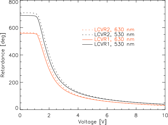
LCVRs are electro-optical tunable retarders made of liquid crystal molecules enclosed between two glass plates. Without an external electric field, all molecules are aligned with their long axis parallel to the glass substrate and maximum retardance is achieved. If an external alternating electrical field is applied (square wave, 2 kHz), the molecules begin to tilt perpendicular to the glass substrate, which causes a reduction of the effective birefringence. The VIP LCVRs can be used in the range from 420 to 700 nm; their retardance was measured as a function of the applied voltage for two wavelengths (530 nm and 630 nm, see Fig. 2). The voltage needed for a specific retardance and wavelength is then derived by a linear interpolation of the calibration curves (Kentischer 2005). At low voltages, the interaction forces within the crystals are the dominant effects. Therefore their relaxation time is longest in this regime (up to 60 ms). To give the LCVRs enough time to reach the desired retardance, the modulation sequence of VIP was chosen such that these transitions occur when the instrument is busy with etalon settings, camera readout, or disk writing.
Dual-beam polarimetry is achieved using a Wollaston prism before the
camera lens L5a and the detector (see Fig. 1, zoom-in
area). It is oriented parallel to the fast axis of the first LCVR and
acts as a polarization analyzer. The two orthogonal beams generated
by the Wollaston are imaged simultaneously onto the same detector. In
the data reduction process, they are combined to minimize
seeing-induced crosstalk (Lites 1987). To reduce image
distortions between the two beams, the Wollaston is made of calcite
instead of quartz. The splitting angle of the prism, 1.37![]() ,
was optimized to fill the entire CCD.
,
was optimized to fill the entire CCD.
|
Figure 2: Calibration curves of the two LCVRs for the reference wavelengths of 530 nm (black) and 630 nm (red). The voltage was increased in steps of 0.02 V. |
| Open with DEXTER | |
2.2 Detectors
The PixelVision Pluto cameras used for TESOS were replaced in 2006.
The new detector system consists of two 16-bit, high frame rate
PhotonMax CCD cameras manufactured by Princeton Instruments/Acton.
Dark current is minimized by thermo-electrical cooling down to
![]() C. The CCD image sensor is a backside illuminated,
C. The CCD image sensor is a backside illuminated,
![]() pixel array (e2v CCD97) with frame transfer technology
and a square pixel size of 16
pixel array (e2v CCD97) with frame transfer technology
and a square pixel size of 16 ![]() m. The wide dynamic range, large
full-well capacity (200 ke- in traditional amplification mode)
and high quantum efficiency (>60% in the wavelength range
400-850 nm) of the cameras make them ideal for spectropolarimetry.
m. The wide dynamic range, large
full-well capacity (200 ke- in traditional amplification mode)
and high quantum efficiency (>60% in the wavelength range
400-850 nm) of the cameras make them ideal for spectropolarimetry.
As a consequence of the different array and pixel size of the new
detector, the imaging optics in the narrow-band channel of TESOS
had to be changed in order to allow for a FOV of about 40
![]() in diameter, while maintaining the pixel scale. The optimum
result was achieved with a f = 169.7 mm lens, which provides
a pixel scale of 0
in diameter, while maintaining the pixel scale. The optimum
result was achieved with a f = 169.7 mm lens, which provides
a pixel scale of 0
![]() 086 pixel-1 and a FOV of
086 pixel-1 and a FOV of
![]() in spectropolarimetric mode.
in spectropolarimetric mode.
3 Spectropolarimetric data acquisition
To determine the Stokes vector, VIP takes four images Ij (
![]() )
with the LCVRs in different modulation states.
Following the IMaX strategy
(Martínez Pillet et al. 2004), the retardances of the first and second LCVR
are set to (315
)
with the LCVRs in different modulation states.
Following the IMaX strategy
(Martínez Pillet et al. 2004), the retardances of the first and second LCVR
are set to (315![]() ,
315
,
315![]() ,
225
,
225![]() ,
225
,
225![]() )
and
(305.264
)
and
(305.264![]() ,
54.736
,
54.736![]() ,
125.264
,
125.264![]() ,
234.736
,
234.736![]() ),
respectively. This results in four linearly independent combinations
),
respectively. This results in four linearly independent combinations
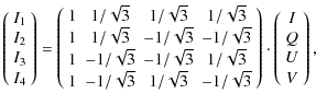
from which the Stokes I, Q, U and V parameters at the position of the LCVRs can be derived.
The theoretical efficiencies are
![]() ,
with
,
with
![]() .
This provides the best modulation possible with
equal efficiency in all Stokes parameters
(del Toro Iniesta & Collados 2000). The polarimeter can also be used to
measure only Stokes I and V; the retardances of the LCVRs are then
(
.
This provides the best modulation possible with
equal efficiency in all Stokes parameters
(del Toro Iniesta & Collados 2000). The polarimeter can also be used to
measure only Stokes I and V; the retardances of the LCVRs are then
(![]() ,
,
![]() )
and (
)
and (![]() ,
,
![]() ), respectively. To
improve the SNR, multiple images for each modulation state can be
accumulated by the control software. Up to now, we have used this
option only to obtain flat field data, since the extra read-out time
increases significantly the duration of the wavelength scans;
for observations, we use long exposures and the large full-well
capacity of the CCDs to reach a sufficiently high SNR.
), respectively. To
improve the SNR, multiple images for each modulation state can be
accumulated by the control software. Up to now, we have used this
option only to obtain flat field data, since the extra read-out time
increases significantly the duration of the wavelength scans;
for observations, we use long exposures and the large full-well
capacity of the CCDs to reach a sufficiently high SNR.
|
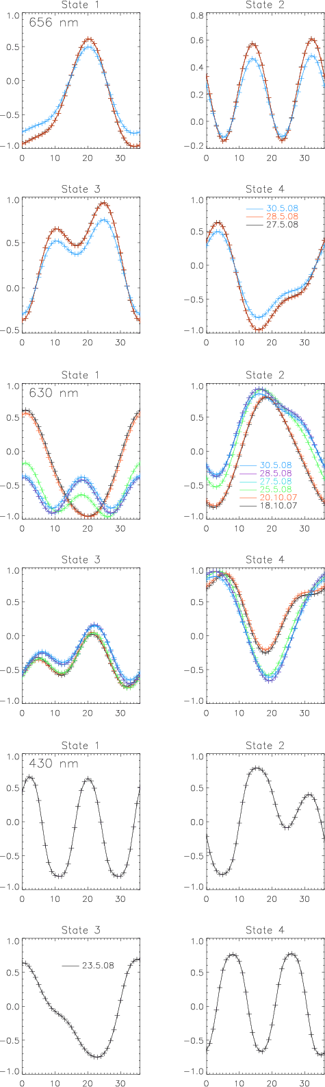
Figure 3: Calibration curves for the four modulation states at 656, 630, and 430 nm (from top to bottom). Calibrations belonging to different days are given in different colors; in some cases the curves are nearly identical and cannot be distinguished from each other (e.g., black and red curve in top four panels). |
| Open with DEXTER | |
4 Data calibration
For the most part, the data reduction process is identical to the one performed when the instrument is operated in spectroscopic mode, which is described in detail elsewhere (see, e.g., Tritschler et al. 2004). The reduction provides flat-fielded and aligned images for each wavelength, modulation state, and orthogonal beam. The alignment of the different scan steps is done using the simultaneous images acquired with the broad-band camera of TESOS (PhotonMax 2 in Fig. 1) as a reference. Here, we only focus on the aspects that are special to spectropolarimetry.
The general approach for the polarimetric calibration of VIP is similar to that of the other spectropolarimeters at the VTT (POLIS, TIP, GFPI). The time-dependent instrumental polarization introduced by the telescope and the remaining optics behind the exit window of the telescope is corrected separately in two steps as described in detail by Beck et al. (2005a), and Schlichenmaier & Collados (2002) or Beck et al. (2005b); for the GFPI see Bello González & Kneer (2008).
To determine the response function, X, of the polarimeter and the
optics behind the instrument calibration unit (ICU), 37 known
polarization states are created by the ICU and measured with VIP (see Fig. 3). The ICU is located right behind the exit
window of the evacuated telescope, and consists of a linear polarizer
and a zero-order quartz retarder. The retarder is rotated in 5![]() steps from 0
steps from 0![]() to 180
to 180![]() ,
with the transmission axis of
the polarizer fixed along the terrestrial N-S direction.
Calibration curves for each of the LCVR states are obtained from the
intensity difference between the two orthogonal beams produced by the
Wollaston, normalized to their average value (Fig. 3).
A flat field correction is not needed for the calibration
measurements, because gain table variations affect the difference and
average images by exactly the same multiplicative factor, and thus they cancel out. Tests
with and without flat field correction yielded the same polarimetric
response down to our accuracy level. The subtraction of the dark
current is, however, crucial because it influences the relative
measurements of intensities in a non-linear way. The four calibration
curves can then be used to determine X by a matrix inversion as
described in Appendix A.2 of Beck et al. (2005b). Applied to the
four intensity measurements that result from subtracting the two
orthogonal beams for each LCVR state, X gives the Stokes parameters
at the position of the ICU.
,
with the transmission axis of
the polarizer fixed along the terrestrial N-S direction.
Calibration curves for each of the LCVR states are obtained from the
intensity difference between the two orthogonal beams produced by the
Wollaston, normalized to their average value (Fig. 3).
A flat field correction is not needed for the calibration
measurements, because gain table variations affect the difference and
average images by exactly the same multiplicative factor, and thus they cancel out. Tests
with and without flat field correction yielded the same polarimetric
response down to our accuracy level. The subtraction of the dark
current is, however, crucial because it influences the relative
measurements of intensities in a non-linear way. The four calibration
curves can then be used to determine X by a matrix inversion as
described in Appendix A.2 of Beck et al. (2005b). Applied to the
four intensity measurements that result from subtracting the two
orthogonal beams for each LCVR state, X gives the Stokes parameters
at the position of the ICU.
VIP differs from slit spectropolarimeters in its 2D FOV, which implies that also the polarization properties can vary in both spatial dimensions. We investigated the derived response functions for subfields of the VIP FOV, but found no significant spatial variation within the accuracy of X. Therefore we use the same response function for every CCD pixel. We also found no significant trend with wavelength inside the typical range used to scan a line, so we compute X only for the first wavelength position (usually a continuum point).
|
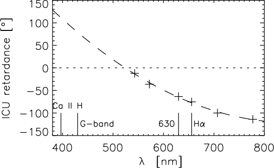
Figure 4: Retardance of the visible ICU at the VTT. Crosses denote measurements, the dashed line a parabolic fit. |
| Open with DEXTER | |
TESOS, and hence VIP, is prepared for sequential multi-wavelength observations. This means that the calibration has to be done for as many spectral regions as used in the observations, but a calibration data set can be taken in less than 15 minutes. The variation of the ICU retardance with wavelength is shown in Fig. 4. The parameters of a parabolic fit to the measured retardances are (688, -1.89537, 0.00110836) for the offset, slope, and 2nd order contribution. The chromatic wave plate of the ICU has zero retardance around 520 nm and cannot be used in this spectral region.
A critical issue for the accuracy of the measurements is the stability
of the polarization modulation over time. We consider here the nematic
LCVRs as the major source of variation, since the remainder of the
setup consists of ``stable'' massive objects like mirrors, the FPIs,
the Wollaston, or beam splitters (BS) that feed additional imaging
channels in front of TESOS. The LCVRs can change the polarimetric
response of the instrument since their effective retardance is
temperature dependent. The retardance decreases by about 1 degree
for an increase in temperature by 1 K (see, e.g., Heredero et al. 2007, their Fig. 5). Measurements at the ICU retarder showed a temperature increase of about 0.6![]() in two minutes on being exposed to sunlight before the temperature leveled off, as well as a reduction of retardance by 0.4
in two minutes on being exposed to sunlight before the temperature leveled off, as well as a reduction of retardance by 0.4![]() at 630 nm comparing measurements in the early morning and at noon (Beck 2004).
The light absorption of the LCVRs, and hence, their behavior, should be
similar. During the observations, the LCVRs are permanently exposed to
the sunlight, since no shutters or similar devices are located in front
of them. There should thus only be some minor and fast heating effect
before the start of the first observation in the early morning and a
slight drift with time caused by the change of the light level during
the day.
at 630 nm comparing measurements in the early morning and at noon (Beck 2004).
The light absorption of the LCVRs, and hence, their behavior, should be
similar. During the observations, the LCVRs are permanently exposed to
the sunlight, since no shutters or similar devices are located in front
of them. There should thus only be some minor and fast heating effect
before the start of the first observation in the early morning and a
slight drift with time caused by the change of the light level during
the day.
Table 1:
Overview of the observations. ![]() :
continuum intensity.
:
continuum intensity.
|
Figure 5:
Left panel: pore data taken in 2005. Bottom
row, left to right: continuum intensity |
| Open with DEXTER | |
The LVCRs of VIP are not located in a temperature-controlled housing,
but the observing room as a whole is air-conditioned with a nominal
temperature of 21 ![]() C.
Temperature changes of the surrounding air will presumably not exceed a
level of one degree due to the air-condition. Taking one degree of
temperature and thus one degree of retardance as the uppermost limit of
variation, this translates into a deviation from the default modulation
scheme by about three percent (e.g.,
C.
Temperature changes of the surrounding air will presumably not exceed a
level of one degree due to the air-condition. Taking one degree of
temperature and thus one degree of retardance as the uppermost limit of
variation, this translates into a deviation from the default modulation
scheme by about three percent (e.g.,
![]() /
/
![]() ).
This three percent is, however, not an absolute but a relative error;
for instance for a polarization signal with an amplitude of 10% of the
continuum intensity, the resulting error would be only 0.3%. Such an
error level is comparable to the rms noise of the data (see Table 1).
The value of the rms noise actually implies that any short-term
variations of temperature on the order of a few seconds cannot reach
one degree, since it provides an upper limit for the contributions of all
noise sources in addition to the thermal retardance effects. The main
effect of the temperature changes will thus be a slow drift of
retardance with time that presumably can be neglected for the
polarimetric accuracy if the calibration is done right before or after
the observations.
).
This three percent is, however, not an absolute but a relative error;
for instance for a polarization signal with an amplitude of 10% of the
continuum intensity, the resulting error would be only 0.3%. Such an
error level is comparable to the rms noise of the data (see Table 1).
The value of the rms noise actually implies that any short-term
variations of temperature on the order of a few seconds cannot reach
one degree, since it provides an upper limit for the contributions of all
noise sources in addition to the thermal retardance effects. The main
effect of the temperature changes will thus be a slow drift of
retardance with time that presumably can be neglected for the
polarimetric accuracy if the calibration is done right before or after
the observations.
In order to verify the stability of the calibration, we collected calibration curves from several campaigns for wavelengths of 430 nm, 630 nm, and 656 nm (Fig. 3). The curves demonstrate that the calibration is stable to within the measurement accuracy for up to two-three days (e.g., 630 nm on October 18 and 20, 2007 or 656 nm on May 27 and 28, 2008). The large changes in the shape of the curves (compare 2007 (red) and 2008 (blue) in state 1, 630 nm) are due to the additional BS used in 2008 to feed the imaging channels; the minor changes between, e.g., May 25 and 30 were due to a re-adjustment of the same BS. We conclude that daily calibration measurements should suffice to maintain a high polarimetric accuracy for VIP if the optical setup remains unchanged.
The measured polarization efficiencies are typically
![]() at
630 nm, slightly below the theoretical values but still very high.
The instrumental polarization caused by the VTT coelostat is
removed using the telescope model of Beck et al. (2005a). If the
polarization level in a continuum window inside the observed spectral
range differs from zero, a correction for residual
at
630 nm, slightly below the theoretical values but still very high.
The instrumental polarization caused by the VTT coelostat is
removed using the telescope model of Beck et al. (2005a). If the
polarization level in a continuum window inside the observed spectral
range differs from zero, a correction for residual
![]() crosstalk is applied by calculating the average QUV/I ratio in the
continuum window and subtracting the corresponding fraction of the
intensity profile from QUV. This
crosstalk comes from two sources of calibration inaccuracies: the
limitations of the geometrical telescope model and the high
sensitivity of the first column of the response matrix to the
retardance adopted for the ICU (see Fig. 4 of Beck et
al. 2005b). The latter quickly leads to deviations of some percent
(roughly 1% of crosstalk per
crosstalk is applied by calculating the average QUV/I ratio in the
continuum window and subtracting the corresponding fraction of the
intensity profile from QUV. This
crosstalk comes from two sources of calibration inaccuracies: the
limitations of the geometrical telescope model and the high
sensitivity of the first column of the response matrix to the
retardance adopted for the ICU (see Fig. 4 of Beck et
al. 2005b). The latter quickly leads to deviations of some percent
(roughly 1% of crosstalk per ![]() error in retardance). The
determination of the ICU retardance can be improved with additional
calibration data at different polarizer positions as described by
Beck et al. (2005b).
error in retardance). The
determination of the ICU retardance can be improved with additional
calibration data at different polarizer positions as described by
Beck et al. (2005b).
5 Observations
After commissioning, VIP has been used in several campaigns from 2005
until 2009. During the first test runs, VIP was a stand-alone
instrument devoted to the observation of the pair of Fe I lines
at 630 nm. In later campaigns it has been operated simultaneously with
TIP and additional imaging channels as, for example, the G-band at
430.5 nm and H![]() (see, e.g., Kucera et al. 2008). In the
following we describe and discuss three specific observations with VIP
to demonstrate its scientific potential. Details of the observations
are given in Table 1.
(see, e.g., Kucera et al. 2008). In the
following we describe and discuss three specific observations with VIP
to demonstrate its scientific potential. Details of the observations
are given in Table 1.
When coordinated with TIP, the spectrograph slit (of length
70
![]() -80
-80
![]() )
was oriented parallel to the long axis of the VIP
FOV, covering it completely. In the direction perpendicular to the
slit the coverage depends on the region scanned with TIP. The setup
for multi-instrument observations including VIP is described in
Beck et al. (2007) and Kucera et al. (2008).
)
was oriented parallel to the long axis of the VIP
FOV, covering it completely. In the direction perpendicular to the
slit the coverage depends on the region scanned with TIP. The setup
for multi-instrument observations including VIP is described in
Beck et al. (2007) and Kucera et al. (2008).
All observations are dark subtracted, flat fielded, and corrected for
transparency fluctuations during the scan. For the two data sets of
network no de-stretch prior to the polarization calibration has been
performed. Usually the observations are binned by a factor of two to
increase the signal-to-noise ratio, so the effective pixel size is
0
![]() 17.
17.
5.1 Pore observations
On November 3, 2005 we observed a pore (NOAA 10818) close to disk
center. VIP was used to scan the two Fe I
630.2 nm lines
sequentially with a total of 88 wavelength points and a scan
time of about 65 s for each line. For the following, we only considered
the line at 630.25nm. In order to determine reliable magnetic
parameters and to assess the performance of VIP, the Stokes I, Q, U and V profiles were inverted using the SIR code. We performed a 1-component
inversion with a variable stray light contribution ![]() fitted by
the algorithm. Depending on whether the polarization signal exceeded
a threshold of 0.85% of the continuum intensity or not, either a
single magnetic or a field-free atmosphere was assumed.
fitted by
the algorithm. Depending on whether the polarization signal exceeded
a threshold of 0.85% of the continuum intensity or not, either a
single magnetic or a field-free atmosphere was assumed.
|
Figure 6:
Left panel: network data taken in 2007. Bottom
to top: |
| Open with DEXTER | |
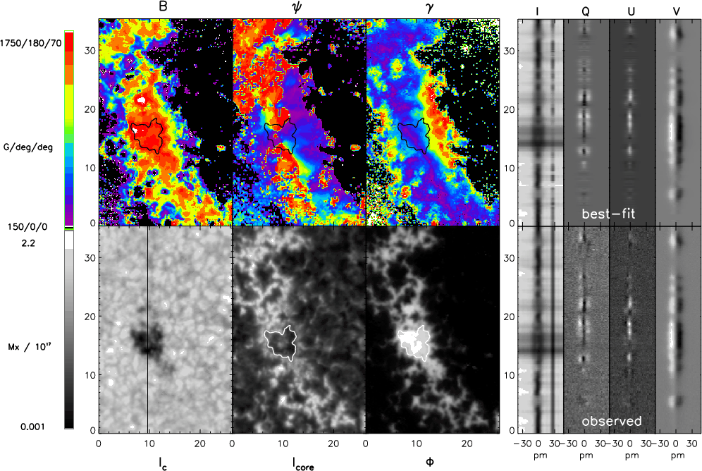
Figure 5 displays the observed FOV (bottom panels)
and some of the inversion results (top panels). The continuum
intensity (bottom left) shows clear signs of abnormal
granulation surrounding the pore. The line-core intensity image
(bottom middle) reveals brightenings that closely follow the
course of the intergranular lanes throughout most of the FOV. The
spatial resolution is sufficient to distinguish the ribbon-like
appearance of these structures, discovered by Berger et al. (2004)
in G-band filtergrams taken at the Swedish 1-m Solar Telescope. A
comparison with the unsigned magnetic flux
![]() (bottom right)
demonstrates that all the
strong line-core brightenings are related to the presence of magnetic
fields. This does not immediately imply that the upper layers of
magnetic
elements are hotter than their surroundings, as not only the
temperature but
also the Zeeman splitting or the shift of the optical depth scale in
the presence of magnetic fields increase the line-core intensity. The
flux concentrations reside predominantly in the intergranular
lanes. The field strength (top left) ranges from 50 G to about
2 kG. The field azimuth (top middle) and field inclination
(top right) indicate radially oriented magnetic fields that
extend well beyond the visible border of the pore (white/black contours). The inclination
increases with radial distance from the center of the pore, reaching a
maximum of about 70
(bottom right)
demonstrates that all the
strong line-core brightenings are related to the presence of magnetic
fields. This does not immediately imply that the upper layers of
magnetic
elements are hotter than their surroundings, as not only the
temperature but
also the Zeeman splitting or the shift of the optical depth scale in
the presence of magnetic fields increase the line-core intensity. The
flux concentrations reside predominantly in the intergranular
lanes. The field strength (top left) ranges from 50 G to about
2 kG. The field azimuth (top middle) and field inclination
(top right) indicate radially oriented magnetic fields that
extend well beyond the visible border of the pore (white/black contours). The inclination
increases with radial distance from the center of the pore, reaching a
maximum of about 70![]() to the LOS. As the pore was located close
to disk center, the corresponding orientation in the local reference
frame (i.e., with respect to the local surface normal) will not differ
much from the LOS values. In the right half of
Fig. 5, the observed and best-fit spectra along a cut
through the pore are shown for comparison.
to the LOS. As the pore was located close
to disk center, the corresponding orientation in the local reference
frame (i.e., with respect to the local surface normal) will not differ
much from the LOS values. In the right half of
Fig. 5, the observed and best-fit spectra along a cut
through the pore are shown for comparison.
We conclude that because of the fine spectral sampling and the high SNR achieved, the spectra can be well analyzed with the SIR code, allowing for an accurate determination of the magnetic field parameters at high spatial resolution. A preliminary investigation of the effect of the transmission profile of TESOS on the observed spectra, mainly using the telluric oxygen line, suggested systematic variations of line widths or line positions across the FOV of 0.1-0.2 pm (see also Puschmann et al. 2006; Reardon & Cavallini 2008; von der Lühe & Kentischer 2000; Martínez Pillet et al. 2004; Scharmer 2006; Tritschler et al. 2002). This translates into an error in the field strength (velocity) of 50 G (50 ms-1) at 630 nm, which is comparable to the error in the determination of the velocity or the magnetic field strength (see, e.g., Beck 2006) and far below their intrinsic variation across the solar surface. A more detailed discussion of the instrumental effects on the retrieved physical parameters is postponed to a future publication.
5.2 Network observations
The network observations taken on October 18, 2007 at about
10:00 UT
were coordinated with TIP. A broad-band G-band speckle channel was
added in front of TESOS to provide context information with high
spatial resolution. TIP was set to repeatedly scan a small region of ![]() 5
5
![]() near the centre of the VIP FOV
near the centre of the VIP FOV![]() .
.
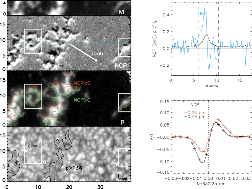
Figure 6 summarizes the observations: the continuum
intensity ![]() (bottom left), the polarization degree
p (middle left), and the net circular polarization (NCP;
top left) in the Fe I line at 630.25 nm. The NCP was
computed as the integral of Stokes V over wavelength, multiplied by
the polarity of the field. The polarization degree was determined as
(bottom left), the polarization degree
p (middle left), and the net circular polarization (NCP;
top left) in the Fe I line at 630.25 nm. The NCP was
computed as the integral of Stokes V over wavelength, multiplied by
the polarity of the field. The polarization degree was determined as
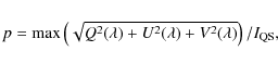
|
(2) |
with
|
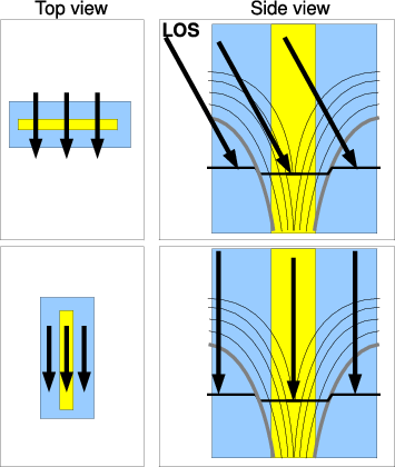
Figure 7: Dependence of NCP behavior on the orientation of magnetic flux sheets. For an orientation of the sheet parallel to the limb ( top row), the inclined LOS passes through both the central part (yellow) and the canopy (blue), for an orientation perpendicular to the limb ( bottom row), it passes through either the canopy or the central axis. The LOS is inclined out of the paper plane in all but the upper right panel. |
| Open with DEXTER | |
The NCP map reveals a distinct pattern, varying between positive and negative values on small spatial scales (e.g., left white rectangle, a). Negative NCP (black) appears preferentially toward the disk center and positive NCP (white) toward the limb. The polarization degree map shows that the highest NCP values are not cospatial with the highest polarization degree, but rather flank it. The effect is visualized in the right panel that shows NCP and p values on a cut along the y-axis through the right white rectangle, b. The NCP reduces to zero and changes sign across the maximum of the polarization degree. The Stokes V profiles corresponding to maximal positive and negative NCP in the cut are shown at the bottom right; the pronounced asymmetry of the red and blue V lobe is clearly visible in the two cases. The spectral sampling is indicated by the crosses.
Figure 7 offers a tentative explanation of how
the peculiar NCP pattern could possibly be created. In the case
of a flux sheet that is parallel to the limb, the LOS crosses
both the canopy and the center of the sheet (top row). If the
flux concentration is perpendicular to the limb (bottom
row), the LOS passes through either the canopy or the
central axis. This scenario provides fairly different gradients of
magnetic field strength along the LOS. In addition, velocity
gradients will presumably be encountered by the LOS at the
boundary of the flux concentration; the field-free convective
region below the canopy and the magnetic volume are expected to
harbor upflows and downflows, respectively. With these velocity
gradients, the two necessary conditions for generating a
NCP are present (see, e.g., Sánchez Almeida & Lites 1992; Auer & Heasley 1978; Landolfi & Landi Degl'Innocenti 1996).
The scenario, however, will have to be investigated in more detail
before it can be taken for plausible. The detection of the variation
of the NCP across magnetic flux concentrations has been
possible thanks to the higher spatial resolution of VIP (or
Hinode, Rezaei et al. 2007) compared to older data where the
resolution was not sufficient to separate the canopy from the
central axis (see, e.g., Sigwarth 2001). Interestingly, a
variation of the Stokes V area asymmetry across magnetic
elements was inferred from the inversion of ASP measurements at 1
![]() (Bellot Rubio et al. 2000).
(Bellot Rubio et al. 2000).
5.3 Network observations in the G band
VIP was used for spectropolarimetry in the G band on May 23, 2008. The
wavelength range covered several CH lines and one strong atomic
line near 430.32 nm. The short wavelength of the observations led to
a rather low average intensity of about 490 counts, but the rms noise
in the polarization signal stayed at about 0.3%. Again, VIP was
operated in coordination with TIP and an external speckle G-band
channel![]() .
.
|
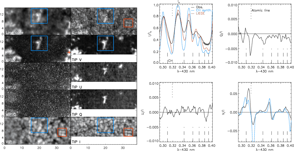
Figure 8:
Left panel: 2008 G-band observations. Left
column, bottom to top: Stokes I and wavelength-integrated
absolute QUV, and line-core intensity near 430.39 nm, as measured
by VIP. Right column, bottom to top: Stokes I and
wavelength-integrated absolute QUV signals from TIP, and
speckle-reconstructed broad-band G-band image. The blue and
red rectangles identify the features used for the data
alignment. The black contours outline large V signals in
TIP. The red cross in the circular polarization map from VIP
near (40
|
| Open with DEXTER | |
Figure 8 shows an overview of the VIP and TIP
observations of a network region located at
![]() ), i.e.,
), i.e.,
![]() away from the disk center. In this case, the two instruments
covered a similar FOV. The ``continuum'' intensity for VIP was taken
at 430.33 nm, where the intensity in the observed wavelength range is
maximum. VIP did not reveal clear Stokes Q and U signals above the noise
level, in contrast to TIP. This may partly be attributed to the different
type of lines observed, the different spectral regions, or the
different SNRs achieved. The V signals of both instruments, however, match closely.
away from the disk center. In this case, the two instruments
covered a similar FOV. The ``continuum'' intensity for VIP was taken
at 430.33 nm, where the intensity in the observed wavelength range is
maximum. VIP did not reveal clear Stokes Q and U signals above the noise
level, in contrast to TIP. This may partly be attributed to the different
type of lines observed, the different spectral regions, or the
different SNRs achieved. The V signals of both instruments, however, match closely.
The Stokes profiles recorded by VIP can be used for quantitative analyses even at the low light level prevailing in the blue. The right panel of Fig. 8 shows sample spectra from a relatively strong flux concentration marked with a red cross in the Stokes V map of VIP. Besides studying how the depth of the various CH lines in Stokes I depends on the physical properties of the plasma and the magnetic field, the observed Stokes V profiles (bottom right) can be used to verify theoretical models of CH line formation. The overplotted blue line comes from a numerical calculation by Uitenbroek et al. (2004), for a height-independent field strength of 1 kG. The V signal was scaled down by a factor of 1.5 to better reproduce the observed CH lines redward of 430.36 nm. The large mismatch between observed and synthetic profiles around 430.31 nm is presumably caused by the parameters used to synthesize the atomic line of Fe II (A. Asensio Ramos, priv. comm.).
6 Summary
The KIS/IAA Visible Imaging Polarimeter (VIP) is a new instrument for
2D spectropolarimetry of the solar atmosphere. It is used with TESOS,
the triple etalon spectrometer installed at the German Vacuum Tower
Telescope. The polarimeter is based on a pair of nematic liquid
crystal retarders and a Wollaston prism. In combination with the
adaptive optics system of the telescope, VIP and TESOS provide full
Stokes vector measurements of spectral lines in the visible at a
resolution of 0
![]() 5 or better. Using exposure times of 300 ms for
each modulation state and
5 or better. Using exposure times of 300 ms for
each modulation state and
![]() binning, the noise level is
about 0.2% of the continuum intensity. The four Stokes profiles can
be measured at 40 wavelength positions in about 60 s. The response
function of the polarimeter is determined using the instrument
calibration unit of the telescope, and turns out to be stable over a
few days.
binning, the noise level is
about 0.2% of the continuum intensity. The four Stokes profiles can
be measured at 40 wavelength positions in about 60 s. The response
function of the polarimeter is determined using the instrument
calibration unit of the telescope, and turns out to be stable over a
few days.
The high resolving power and excellent performance of TESOS and VIP
make it possible to derive the magnetic field geometry and
obtain information about the atmospheric conditions by means of
inversion techniques. The Stokes spectra recorded by VIP show strong
asymmetries, as expected for high-resolution measurements. Thus, it
should be possible to determine vertical gradients of the atmospheric
parameters from them. Photospheric and chromospheric lines (e.g.,
H![]() )
can be observed sequentially thanks to the motorized filter
wheel of TESOS.
)
can be observed sequentially thanks to the motorized filter
wheel of TESOS.
Usually VIP is operated in coordination with the Tenerife Infrared Polarimeter and speckle imaging systems at the German Vacuum Tower Telescope, providing multi-wavelength observations of the same structures and processes. VIP could also be used for coordinated observations with space-borne instruments such as Hinode or the upcoming Solar Dynamic Observatory. Because of these reasons, we anticipate that future observations with VIP will be used to address several open questions in solar physics.
AcknowledgementsThe VTT is operated by the Kiepenheuer-Institut für Sonnenphysik, Freiburg, Germany, at the Spanish Observatorio del Teide of the Instituto de Astrofísica de Canarias. This work has been partially funded by the Spanish Ministerio de Ciencia e Innovación through project ESP2006-13030-C06-02 (including European FEDER funds) and through project AYA 2007-63881.
References
- Álvarez-Herrero, A., Belenguer, T., Pastor, C., et al. 2006, in SPIE Conf. Ser. 6265, ed. J. C. Mather, H. A. MacEwen, & M. W. M. de Graauw, 132 [Google Scholar]
- Auer, L. H., & Heasley, J. N. 1978, A&A, 64, 67 [NASA ADS] [Google Scholar]
- Beck, C. 2004, Technical note, Kiepenheuer Institut für Sonnenphysik, Freiburg [Google Scholar]
- Beck, C. 2006, Ph.D. Thesis, Albert-Ludwigs-University, Freiburg [Google Scholar]
- Beck, C., & Rezaei, R. 2009, A&A, 502, 969 [NASA ADS] [CrossRef] [EDP Sciences] [Google Scholar]
- Beck, C., Schlichenmaier, R., Collados, M., Bellot Rubio, L., & Kentischer, T. 2005a, A&A, 443, 1047 [NASA ADS] [CrossRef] [EDP Sciences] [Google Scholar]
- Beck, C., Schmidt, W., Kentischer, T., & Elmore, D. 2005b, A&A, 437, 1159 [NASA ADS] [CrossRef] [EDP Sciences] [Google Scholar]
- Beck, C., Mikurda, K., Bellot Rubio, L. R., Kentischer, T., & Collados, M. 2007, in Modern solar facilities - advanced solar science, ed. F. Kneer, K. G. Puschmann, & A. D. Wittmann, 55 [Google Scholar]
- Beck, C., Schmidt, W., Rezaei, R., & Rammacher, W. 2008, A&A, 479, 213 [NASA ADS] [CrossRef] [EDP Sciences] [Google Scholar]
- Bello González, N., & Kneer, F. 2008, A&A, 480, 265 [NASA ADS] [CrossRef] [EDP Sciences] [Google Scholar]
- Bellot Rubio, L. R., Ruiz Cobo, B., & Collados, M. 2000, ApJ, 535, 489 [NASA ADS] [CrossRef] [Google Scholar]
- Bellot Rubio, L. R., Schlichenmaier, R., & Tritschler, A. 2006, A&A, 453, 1117 [NASA ADS] [CrossRef] [EDP Sciences] [Google Scholar]
- Berger, T. E., Rouppe van der Voort, L. H. M., Löfdahl, M. G., et al. 2004, A&A, 428, 613 [NASA ADS] [CrossRef] [EDP Sciences] [Google Scholar]
- Bommier, V., & Molodij, G. 2002, A&A, 381, 241 [NASA ADS] [CrossRef] [EDP Sciences] [Google Scholar]
- Carlsson, M., & Stein, R. F. 1997, ApJ, 481, 500 [Google Scholar]
- Cavallini, F. 2006, Sol. Phys., 236, 415 [NASA ADS] [CrossRef] [Google Scholar]
- Collados, M., Lagg, A., Díaz García, J. J., et al. 2007, in The Physics of Chromospheric Plasmas, ed. P. Heinzel, I. Dorotovic, & R. J. Rutten, ASP Conf. Ser., 368, 611 [Google Scholar]
- del Toro Iniesta, J. C., & Collados, M. 2000, Appl. Opt., 39, 1637 [NASA ADS] [CrossRef] [PubMed] [Google Scholar]
- Gandorfer, A. M., Solanki, S. K., Barthol, P., et al. 2006, in SPIE Conf. Ser., ed. L. M. Stepp, 6267, 25 [Google Scholar]
- Heredero, R. L., Uribe-Patarroyo, N., Belenguer, T., et al. 2007, Appl. Opt., 46, 689 [NASA ADS] [CrossRef] [PubMed] [Google Scholar]
- Jaeggli, S. A., Lin, H., Mickey, D. L., et al. 2008, AGU Spring Meeting Abstracts, A11 [Google Scholar]
- Jochum, L., Collados, M., Martínez Pillet, V., et al. 2003, in SPIE Conf. Ser., ed. S. Fineschi, 4843, 20 [Google Scholar]
- Keller, C. U., & von der Luehe, O. 1992, A&A, 261, 321 [NASA ADS] [Google Scholar]
- Kentischer, T. 2005, Technical note, Kiepenheuer Institut für Sonnenphysik, Freiburg [Google Scholar]
- Kentischer, T. J., Schmidt, W., Sigwarth, M., & von Uexküll, M. 1998, A&A, 340, 569 [NASA ADS] [Google Scholar]
- Khomenko, E. V., Collados, M., Solanki, S. K., Lagg, A., & Trujillo Bueno, J. 2003, A&A, 408, 1115 [NASA ADS] [CrossRef] [EDP Sciences] [Google Scholar]
- Kosugi, T., Matsuzaki, K., Sakao, T., et al. 2007, Sol. Phys., 243, 3 [NASA ADS] [CrossRef] [Google Scholar]
- Kucera, A., Beck, C., Gomory, P., et al. 2008, 12th European Solar Physics Meeting, Freiburg, Germany, held September 8-12, http://espm.kis.uni-freiburg.de/, 12, 2 [Google Scholar]
- Landolfi, M., & Landi Degl'Innocenti, E. 1996, Sol. Phys., 164, 191 [NASA ADS] [CrossRef] [Google Scholar]
- Langhans, K., Schmidt, W., & Tritschler, A. 2002, A&A, 394, 1069 [NASA ADS] [CrossRef] [EDP Sciences] [Google Scholar]
- Lites, B. W. 1987, Appl. Opt., 26, 3838 [NASA ADS] [CrossRef] [PubMed] [Google Scholar]
- López Ariste, A., Rayrole, J., & Semel, M. 2000, A&AS, 142, 137 [Google Scholar]
- Martínez González, M. J., Collados, M., Ruiz Cobo, B., & Beck, C. 2008, A&A, 477, 953 [NASA ADS] [CrossRef] [EDP Sciences] [Google Scholar]
- Martínez Pillet, V., Collados, M., Sánchez Almeida, J., et al. 1999, in ASP Conf. Ser., 183, 264 [Google Scholar]
- Martínez Pillet, V., Bonet, J. A., Collados, M. V., et al. 2004, in SPIE Conf. Ser. 5487, ed. J. C. Mather, 1152 [Google Scholar]
- Mickey, D. L., Canfield, R. C., Labonte, B. J., et al. 1996, Sol. Phys., 168, 229 [Google Scholar]
- Mikurda, K., Tritschler, A., & Schmidt, W. 2006, A&A, 454, 359 [NASA ADS] [CrossRef] [EDP Sciences] [Google Scholar]
- Puschmann, K. G., & Sailer, M. 2006, A&A, 454, 1011 [NASA ADS] [CrossRef] [EDP Sciences] [Google Scholar]
- Puschmann, K. G., Kneer, F., Seelemann, T., & Wittmann, A. D. 2006, A&A, 451, 1151 [NASA ADS] [CrossRef] [EDP Sciences] [Google Scholar]
- Rayrole, J., & Mein, P. 1993, in The Magnetic and Velocity Fields of Solar Active Regions, ed. H. Zirin, G. Ai, & H. Wang, IAU Colloq., 141, ASP Conf. Ser., 46, 170 [Google Scholar]
- Reardon, K. P., & Cavallini, F. 2008, A&A, 481, 897 [NASA ADS] [CrossRef] [EDP Sciences] [Google Scholar]
- Rezaei, R., Steiner, O., Wedemeyer-Böhm, S., et al. 2007, A&A, 476, L33 [NASA ADS] [CrossRef] [EDP Sciences] [Google Scholar]
- Rimmele, T. R. 2004, in SPIE Conf. Ser. 5490, ed. D. Bonaccini Calia, B. L. Ellerbroek, & R. Ragazzoni, 34 [Google Scholar]
- Rutten, R. J., & Uitenbroek, H. 1991, Sol. Phys., 134, 15 [NASA ADS] [CrossRef] [Google Scholar]
- Sánchez Almeida, J., & Lites, B. W. 1992, ApJ, 398, 359 [NASA ADS] [CrossRef] [Google Scholar]
- Sankarasubramanian, K., Elmore, D. F., Lites, B. W., et al. 2003, in SPIE Conf. Ser. 4843, ed. S. Fineschi, 414 [Google Scholar]
- Scharmer, G. B. 2006, A&A, 447, 1111 [NASA ADS] [CrossRef] [EDP Sciences] [Google Scholar]
- Scharmer, G. B., Dettori, P. M., Lofdahl, M. G., & Shand, M. 2003, in SPIE Conf. Ser. 4853, ed. S. L. Keil, & S. V. Avakyan, 370 [Google Scholar]
- Scharmer, G. B., Narayan, G., Hillberg, T., et al. 2008, ApJ, 689, L69 [NASA ADS] [CrossRef] [Google Scholar]
- Schleicher, H., Wöhl, H., & Balthasar, H. 2003, Astron. Nachr. Suppl., 324, 114 [NASA ADS] [Google Scholar]
- Schlichenmaier, R., & Collados, M. 2002, A&A, 381, 668 [NASA ADS] [CrossRef] [EDP Sciences] [Google Scholar]
- Schlichenmaier, R., & Schmidt, W. 1999, A&A, 349, L37 [NASA ADS] [Google Scholar]
- Schlichenmaier, R., Bellot Rubio, L. R., & Tritschler, A. 2004, A&A, 415, 731 [NASA ADS] [CrossRef] [EDP Sciences] [Google Scholar]
- Schmidt, W., & Schlichenmaier, R. 2000, A&A, 364, 829 [NASA ADS] [Google Scholar]
- Sigwarth, M. 2001, ApJ, 563, 1031 [NASA ADS] [CrossRef] [Google Scholar]
- Skumanich, A., Lites, B. W., Martínez Pillet, V., & Seagraves, P. 1997, ApJS, 110, 357 [NASA ADS] [CrossRef] [Google Scholar]
- Socas-Navarro, H., Elmore, D., Pietarila, A., et al. 2006, Sol. Phys., 235, 55 [NASA ADS] [CrossRef] [Google Scholar]
- Tritschler, A., Schmidt, W., Langhans, K., & Kentischer, T. 2002, Sol. Phys., 211, 17 [NASA ADS] [CrossRef] [Google Scholar]
- Tritschler, A., Schlichenmaier, R., Bellot Rubio, L. R., et al. 2004, A&A, 415, 717 [NASA ADS] [CrossRef] [EDP Sciences] [Google Scholar]
- Uitenbroek, H., Miller-Ricci, E., Asensio Ramos, A., & Trujillo Bueno, J. 2004, ApJ, 604, 960 [NASA ADS] [CrossRef] [Google Scholar]
- van Noort, M., Rouppe van der Voort, L., & Löfdahl, M. G. 2005, Sol. Phys., 228, 191 [NASA ADS] [CrossRef] [Google Scholar]
- von der Lühe, O., & Kentischer, T. J. 2000, A&AS, 146, 499 [NASA ADS] [CrossRef] [EDP Sciences] [Google Scholar]
- von der Lühe, O., Soltau, D., Berkefeld, T., & Schelenz, T. 2003, in SPIE Conf. Ser. 4853, ed. S. L. Keil, & S. V. Avakyan, 187 [Google Scholar]
- Wedemeyer, S., Freytag, B., Steffen, M., Ludwig, H.-G., & Holweger, H. 2004, A&A, 414, 1121 [NASA ADS] [CrossRef] [EDP Sciences] [Google Scholar]
- Wöger, F., Wedemeyer-Böhm, S., Schmidt, W., & von der Lühe, O. 2006, A&A, 459, L9 [NASA ADS] [CrossRef] [EDP Sciences] [Google Scholar]
Footnotes
- ... Peak
![[*]](/icons/foot_motif.png)
- Operated by the Association of Universities for Research in Astronomy, Inc. (AURA), for the National Science Foundation.
- ... FOV
- See the TIP archive for an overview of the TIP data (KIS home
page
 Observatories
Data archives).
Observatories
Data archives).
- ...
channel
- In this observation, the spectral resolution of TESOS was lower than usual because of a mistake in the setup (the parallelism of the FPIs was not adjusted).
All Tables
Table 1:
Overview of the observations. ![]() :
continuum intensity.
:
continuum intensity.
All Figures
|
|
Figure 1:
Optical setup of TESOS in high resolution mode. The light
undergoes four |
| Open with DEXTER | |
| In the text | |
|
|
Figure 2: Calibration curves of the two LCVRs for the reference wavelengths of 530 nm (black) and 630 nm (red). The voltage was increased in steps of 0.02 V. |
| Open with DEXTER | |
| In the text | |
|
|
Figure 3: Calibration curves for the four modulation states at 656, 630, and 430 nm (from top to bottom). Calibrations belonging to different days are given in different colors; in some cases the curves are nearly identical and cannot be distinguished from each other (e.g., black and red curve in top four panels). |
| Open with DEXTER | |
| In the text | |
|
|
Figure 4: Retardance of the visible ICU at the VTT. Crosses denote measurements, the dashed line a parabolic fit. |
| Open with DEXTER | |
| In the text | |
|
|
Figure 5:
Left panel: pore data taken in 2005. Bottom
row, left to right: continuum intensity |
| Open with DEXTER | |
| In the text | |
|
|
Figure 6:
Left panel: network data taken in 2007. Bottom
to top: |
| Open with DEXTER | |
| In the text | |
|
|
Figure 7: Dependence of NCP behavior on the orientation of magnetic flux sheets. For an orientation of the sheet parallel to the limb ( top row), the inclined LOS passes through both the central part (yellow) and the canopy (blue), for an orientation perpendicular to the limb ( bottom row), it passes through either the canopy or the central axis. The LOS is inclined out of the paper plane in all but the upper right panel. |
| Open with DEXTER | |
| In the text | |
|
|
Figure 8:
Left panel: 2008 G-band observations. Left
column, bottom to top: Stokes I and wavelength-integrated
absolute QUV, and line-core intensity near 430.39 nm, as measured
by VIP. Right column, bottom to top: Stokes I and
wavelength-integrated absolute QUV signals from TIP, and
speckle-reconstructed broad-band G-band image. The blue and
red rectangles identify the features used for the data
alignment. The black contours outline large V signals in
TIP. The red cross in the circular polarization map from VIP
near (40
|
| Open with DEXTER | |
| In the text | |
Copyright ESO 2010
Current usage metrics show cumulative count of Article Views (full-text article views including HTML views, PDF and ePub downloads, according to the available data) and Abstracts Views on Vision4Press platform.
Data correspond to usage on the plateform after 2015. The current usage metrics is available 48-96 hours after online publication and is updated daily on week days.
Initial download of the metrics may take a while.