| Issue |
A&A
Volume 520, September-October 2010
Pre-launch status of the Planck mission
|
|
|---|---|---|
| Article Number | A7 | |
| Number of page(s) | 12 | |
| Section | Astronomical instrumentation | |
| DOI | https://doi.org/10.1051/0004-6361/200912891 | |
| Published online | 15 September 2010 | |
Pre-launch status of the Planck mission
Planck pre-launch status: Low Frequency Instrument optics
M. Sandri1 - F. Villa1 - M. Bersanelli2 - C. Burigana1 - R. C. Butler1 - O. D'Arcangelo3 - L. Figini3 - A. Gregorio4,5 - C. R. Lawrence6 - D. Maino2 - N. Mandolesi1 - M. Maris4 - R. Nesti7 - F. Perrotta8 - P. Platania3 - A. Simonetto3 - C. Sozzi3 - J. Tauber9 - L. Valenziano1
1 - INAF-IASF Bologna, via Gobetti 101, 40129 Bologna, Italy
2 - Università degli Studi di Milano, via Celoria 16, 20133 Milano,
Italy
3 - IFP-CNR, via Cozzi 53, Milano, Italy
4 - INAF-OATS, via Tiepolo 11, 34143 Trieste, Italy
5 - University of Trieste, Department of Physics, via Valerio 2, 34127
Trieste, Italy
6 - Jet Propulsion Laboratory, California Institute of Technology, 4800
Oak Grove Drive, Pasadena CA 91109, USA
7 - Osservatorio Astrofisico di Arcetri, INAF, Largo E. Fermi 5, 50125
Florence, Italy
8 - SISSA, via Beirut 4, 34014 Trieste, Italy
9 - ESA ESTEC, PO Box 299, 2200 AG Noordwijk, The Netherlands
Received 14 July 2009 / Accepted 1 October 2009
Abstract
We describe the optical design and optimisation of the Low Frequency
Instrument (LFI), one of two instruments onboard the Planck
satellite, which will survey the cosmic microwave background with
unprecedented accuracy. The LFI covers the 30-70 GHz frequency
range with an array of cryogenic radiometers. Stringent optical
requirements on angular resolution, sidelobes, main beam symmetry,
polarization purity, and feed orientation have been achieved. The
optimisation process was carried out by assuming an ideal telescope
according to the Planck design and by using both
physical optics and multi-reflector geometrical theory of diffraction.
This extensive study led to the flight design of the feed horns, their
characteristics, arrangement, and orientation, while taking into
account the opto-mechanical constraints imposed by complex interfaces
in the Planck focal surface.
Key words: cosmic microwave background - space vehicles: instruments - instrumentation: detectors - submillimeter: general - telescopes
1 Introduction
The Planck![]() Satellite was developed to measure the temperature and polarization of
the cosmic microwave background (CMB) over the entire sky with
unprecedented sensitivity and angular resolution. The Low Frequency
Instrument (LFI), operating in the 30-70 GHz frequency range,
is an array of cryogenic pseudo-correlation radiometers (Bersanelli
et al. 2010) sharing the focal surface of a 1.5 m
off-axis dual reflector telescope with the High Frequency Instrument
(HFI) (see Lamarre et al. 2010). This unique optical layout,
with one instrument (LFI) surrounding the other (HFI), leads to
potentially significant off-axis aberrations in the LFI beams that must
be accurately controlled in the telescope and instrument design
optimization phases. The requirements on the LFI beams were originally
set in terms of angular resolution (33
Satellite was developed to measure the temperature and polarization of
the cosmic microwave background (CMB) over the entire sky with
unprecedented sensitivity and angular resolution. The Low Frequency
Instrument (LFI), operating in the 30-70 GHz frequency range,
is an array of cryogenic pseudo-correlation radiometers (Bersanelli
et al. 2010) sharing the focal surface of a 1.5 m
off-axis dual reflector telescope with the High Frequency Instrument
(HFI) (see Lamarre et al. 2010). This unique optical layout,
with one instrument (LFI) surrounding the other (HFI), leads to
potentially significant off-axis aberrations in the LFI beams that must
be accurately controlled in the telescope and instrument design
optimization phases. The requirements on the LFI beams were originally
set in terms of angular resolution (33![]() ,
24
,
24![]() ,
and 14
,
and 14![]() ,
respectively at 30 GHz, 44 GHz, and 70 GHz)
and straylight contamination (lower than 3
,
respectively at 30 GHz, 44 GHz, and 70 GHz)
and straylight contamination (lower than 3 ![]() K).
The aim of this paper is to describe the complex process of design and
optimization of the LFI optics, leading to the current flight
configuration, which in some cases achieves angular resolutions
superior to the requirements.
K).
The aim of this paper is to describe the complex process of design and
optimization of the LFI optics, leading to the current flight
configuration, which in some cases achieves angular resolutions
superior to the requirements.
A CMB experiment should ideally have an optical system
producing symmetric Gaussian beam responses to avoid distortion
effects, and without spillover, to avoid straylight entering the
detectors through the sidelobes producing signals that may be
indistinguishable from fluctuations in the CMB. In real systems,
however, residual non-idealities in the optical system may introduce
serious limitations to the scientific return if not well understood and
controlled. The systematic effects induced by the optics can be divided
into two main areas: (i) the aberrations of the main beam, which
degrade the angular resolution and increase the uncertainty in the
measurements at high multipoles (particularly for polarization) as the
texture of the cosmic signal is smeared and distorted; (ii) the
sidelobes in the feed/telescope radiation pattern, which contribute to
the straylight induced noise, i.e., the unwanted power reaching the
detectors and not coupled through the main beam. These introduce
contamination mainly at large and intermediate angular scales,
typically at multipoles less than ![]() 100.
100.
In this paper, we present the definition, optimization, and characterization of the LFI optical interfaces. The work involved here has been carried out by means of electromagnetic simulations devoted to maximizing the angular resolution and at the same time minimizing systematic effects. The starting point of the optimization activity was the Planck telescope, which is an off-axis Gregorian telescope satisfying the Mizuguchi-Dragone condition. Initially, the LFI focal surface configuration included (in addition to the frequency channels at 30, 44 and, 70 GHz), also a channel at 100 GHz comprising seventeen horns distributed around the HFI front-end. The LFI 100 GHz channel was subsequently removed, but it was part of the initial study and much of the analysis was completed for this channel and applied to the lower frequencies. The position and orientation of each horn was determined by taking into account the mechanical constraints imposed by the LFI interfaces and 4 K reference loads attached to the HFI instrument (see Mandolesi et al. 2010) and assuming a Gaussian model. We emphasize that the simulations discussed in this paper were carried out by assuming a radio frequency model composed of the ideal telescope, the baffle, and the coldest V-groove thermal radiator (see Sandri et al 2002b). The current most suitable model of the detailed beams for both LFI and HFI, taking into account a realistic model of the telescope, are given in Tauber et al. (2010).
The assumed Planck telescope design and the focal surface layout are described in Sects. 2 and 3, respectively. In Sect. 4, edge-taper degradation of the horns is presented. The edge-taper was degraded to improve the angular resolution while maintaining straylight rejection to within the requirements. Section 5 presents the feedhorn alignment process, complete so that CMB polarization measurements can be made. In Sect. 6, given the edge-taper values and the location and orientation of the feeds detemined in the previous sections, each horn design was then optimized in terms of sidelobe level, cross polarization response, and beamwidth. This optimization was first carried out at 100 GHz, i.e., the most critical channel for LFI, and the results were extrapolated to lower frequencies, taking care to check the consistency at the end of the activity. Finally, the fully optimized performance of the LFI beams is reported in Sect. 7.
2 Telescope optical design
The Planck telescope was designed to comply with
the following high level opto-mechanical requirements: wide frequency
coverage (about two decades), 100 squared degrees of field of
view, wide focal region (
![]() mm), and a cryogenic
operational environment (40- 65 K). These unique
characteristics for an experimental cosmology telescope have never been
previously implemented. The Planck telescope
represents a challenge for telescope technology and optical design
(Villa et al. 2002;
Tauber et al. 2010).
mm), and a cryogenic
operational environment (40- 65 K). These unique
characteristics for an experimental cosmology telescope have never been
previously implemented. The Planck telescope
represents a challenge for telescope technology and optical design
(Villa et al. 2002;
Tauber et al. 2010).
The telescope optical layout is based on a dual reflector
off-axis Gregorian design. This configuration allows it to have a small
overall focal ratio (and thus small feeds), an unobstructed field of
view, and low diffraction effects from the secondary reflector and
struts. It allows, at the same time, the secondary reflector to be
appropriately oversized. To improve the image quality, the design has
been optimized by changing the conic constants, the radius of
curvature, the distance between the mirrors, and the tilting of both
mirrors, using the spillover level and the wave front error as
optimization parameters (Dubruel et al. 2000). The primary
mirror is elliptical in shape (but nearly parabolic since the conic
constant is about -0.9) as in aplanatic configurations (Wilson
1996), and the
size of the rim is ![]() m.
The offset of the primary reflector, i.e., the distance between its
center and its major axis, is 1.04 m, while the secondary
reflector offset is 0.3 m. The secondary mirror is elliptical
with a nearly circular rim about 1 m in diameter.
The overall focal ratio,
m.
The offset of the primary reflector, i.e., the distance between its
center and its major axis, is 1.04 m, while the secondary
reflector offset is 0.3 m. The secondary mirror is elliptical
with a nearly circular rim about 1 m in diameter.
The overall focal ratio, ![]() ,
equals 1.1, and the projected aperture is circular with a
diameter of 1.5 m. The telescope field of view is
,
equals 1.1, and the projected aperture is circular with a
diameter of 1.5 m. The telescope field of view is ![]() 5
5![]() centered on the line of sight (LOS), which is tilted at
about 3.7
centered on the line of sight (LOS), which is tilted at
about 3.7![]() relative to the main reflector axis, and forms an angle of 85
relative to the main reflector axis, and forms an angle of 85![]() with the satellite spin axis, which is typically oriented in the
anti-Sun direction during the survey (Dupac 2008). The Planck
telescope as a complete satellite subsystem is shown in Fig. 1 and a
detailed description is reported in Tauber et al. (2010).
with the satellite spin axis, which is typically oriented in the
anti-Sun direction during the survey (Dupac 2008). The Planck
telescope as a complete satellite subsystem is shown in Fig. 1 and a
detailed description is reported in Tauber et al. (2010).
![\begin{figure}
\par\includegraphics[width=21pc,clip]{images/12891fg1.eps}
\end{figure}](/articles/aa/full_html/2010/12/aa12891-09/img20.png)
|
Figure 1:
Lateral and top view of the telescope unit consisting of the reflectors
and the support structure; the hexagonal support structure is readily
seen as well as the field of view (in gray) (left panel).
The telescope unit allocated into Planck satellite (right
panel). The vertical axis is the spin axis of the satellite
and the line of sight is tilted by |
| Open with DEXTER | |
![\begin{figure}
\par\begin{tabular}{c}
\includegraphics[height=7.5cm,clip]{images...
...ncludegraphics[height=6.3cm,clip]{images/12891fg3.eps}\end{tabular}
\end{figure}](/articles/aa/full_html/2010/12/aa12891-09/img21.png)
|
Figure 2: A CAD model of the Planck focal plane, which is located directly below the telescope primary mirror. It comprises the HFI bolometric detector array (small feed horns on golden circular base) and the LFI radio receiver array (larger feed horns around the HFI). The box holding the feedhorns appears to be transparent in this view, to also show the elements inside and behind it ( top panel). The HFI and LFI feed horns are seen reflected in the primary mirror of the Planck telescope in the clean room at Kourou, French Guiana ( bottom panel). © ESA/Thales. |
| Open with DEXTER | |
3 LFI optical interfaces
In its flight configuration, LFI is coupled to the telescope by eleven dual-profiled, corrugated, conical horns (Villa et al. 2010): six feed horns at 70 GHz (FH18 - FH23), three feed horns at 44 GHz (FH24 - FH26), and two feed horns at 30 GHz (FH27 and FH28). Figure 2 shows the arrangement of the horns inside the LFI main frame. It should be noted that the feed position in the focal surface is axisymmetric (for instance, FH27 is symmetric to FH28 at 30 GHz), a natural design choice based on the symmetry of the telescope and satellite. As a consequence, only six different feed elements have been considered in the optimisation analysis: one feed at 30 GHz, two at 44 GHz, and three at 70 GHz (Villa et al. 2010). The center of the focal surface is occupied by the HFI horns. This optical layout, with one instrument (LFI) around the other (HFI), required that aberration effects in the LFI beams be accurately controlled in the telescope and instrument design optimization phases. Corrugated horns were selected as the most suitable solution in terms of cross polarization levels, sidelobes levels, return and insertion loss. Dual-profiled corrugation shaping was chosen for the control of the main lobe shape, the phase centre location, and compactness (Clarricoats 1984; Olver & Xiang 1988). The corrugation profile of each horn was designed to achieve a trade-off between angular resolution and straylight rejection. Each feed horn is connected to an orthomode transducer (OMT) to divide the field propagating into the horn into two orthogonal linear polarization components, X and Y (D'Arcangelo et al. 2010).
The feeds and corresponding OMTs are adjusted in the focal
surface so that the main beam polarization directions of the two
symmetrically located feed horns in the focal plane unit (FPU) are at
an angle of 45 degrees when observed in the same direction in
the sky. This configuration permits measurement of the Q and U Stokes
parameters and thus the linear polarization of the CMB. The location
and orientation of each horn is reported in Table 1, with respect to
the reference detector plane (RDP) coordinate system, placed in the
center of the FPU and with the ![]() axis aligned along the chief ray of the telescope.
axis aligned along the chief ray of the telescope.
The focal plane configuration is a result of a long iteration
process. Apart from the horn aperture definition, which is the result
of edge-taper optimization (see Sect. 4), the
location, the orientation, and the length of the feed horns were
determined on the basis of the mechanical interfaces, feed mutual
obscuration, and pointing direction as derived form the telescope
characteristics. The horn pointing was obtained from the optical study
of the telescope and the tilting angles were derived by means of ray
tracing simulations. This study was addressed at the end of the
telescope optimization process when the focal plane design was not
frozen. However, this was sufficient to derive analytical formulae for
pointing that have been used in additional focal plane optimizations,
ending with the final design. We consider the reference detector plane
coordinate system ![]() as a starting point to define horn pointing. The horn pointing depends
only on the
as a starting point to define horn pointing. The horn pointing depends
only on the ![]() coordinates, while
coordinates, while ![]() defines the phase centre location only. We also define the two rotation
angles as
defines the phase centre location only. We also define the two rotation
angles as ![]() the rotation angle around
the rotation angle around ![]() ,
and
,
and ![]() the rotation around
the rotation around ![]() axis. For the Planck telescope, and in the region
where the LFI feeds are located (i.e., outside the centre of the focal
plane), the two angles were derived from a linear fit to the optical
simulation results:
axis. For the Planck telescope, and in the region
where the LFI feeds are located (i.e., outside the centre of the focal
plane), the two angles were derived from a linear fit to the optical
simulation results:
|
|
= | (1) | |
| = | (2) |
The lengths of the horns were chosen to satisfy the following constraints: (i) to guarantee the interface specifications of the 4 K reference load (which are attached to the HFI instrument, and are thus a driver on the LFI focal plane interface design); (ii) to guarantee matching with both the focal surface and the obscuration criterion of the LFI horns. These criteria fixed the clearance as a cone of
Table 1: Location and orientation of the LFI feed horns.
4 Edge-taper evaluation
The angular resolution (expressed here in terms of full width half maximum, FWHM) of the beam in the sky depends on the illumination, g(x,y), of the primary mirror. For an aperture-type antenna (such as a reflecting telescope), the far field is the Fourier transform of the aperture illumination function. If a Gaussian illumination is assumed, the main beam shape is Gaussian too. The flatter the illumination, the narrower the resulting pattern; in contrast, if the illumination is more centrally peaked, then the angular resolution of the pattern is degraded. For a dual reflector telescope, the illumination function g(x,y) is produced by the feed-horn pattern, reflected and diffracted by the subreflector, and distorted by aberrations mainly due to the off-axis position of the feeds. This is the case for the LFI focal plane configuration. The trade-off between the angular resolution (which impacts the instrument's ability to reconstruct the anisotropy power spectrum of the cosmic microwave background radiation at high multipoles) and the edge-taper (which controls the systematic effect of straylight radiation) was identified as a critical design step. A preliminary analysis was carried out at the beginning of the optimization activity. The sidelobe level is determined by the edge-taper, which is defined to be the ratio of the power per unit area incident on the centre of the mirror (if the illumination is symmetrical, otherwise the maximum illumination is considered) to that incident at the edge. A strong taper (or a high value of the edge-taper) means a strong illumination beneath the reflector, which has a negative impact on the angular resolution. In contrast, increasing the illumination of the telescope (low values of the edge-taper) improves the angular resolution and degrades the straylight rejection of the telescope. The edge-taper can be modified by changing the feed-horn design, which controls the way in which the horn illuminates the telescope. The dependence of the angular resolution improvement on the edge-taper degradation is almost linear until a threshold is achieved, when increasing the illumination on the primary mirror no longer produces further improvement in the angular resolution. This is because a strong illumination of the mirrors increases the aberrations of the main beam. Obviously, the amount of improvement depends on the feed-horn location, since the primary mirror is illuminated in a different way.
![\begin{figure}
\par\includegraphics[height=9cm,angle=90,clip]{images/12891fg4.ps}
\end{figure}](/articles/aa/full_html/2010/12/aa12891-09/img38.png)
|
Figure 3: Simulated co-polar pattern, in the E- plane, of the FM feed horns at 70 (FH21, FH22, and FH23), 44 (FH24 and FH25), and 30 (FH27) GHz assuming the designed profile. |
| Open with DEXTER | |
| Figure 4: 10 dB contour of all horn patterns on the sub (left panel) and main (right panel) reflectors: the contours corresponding to the 30 GHz patterns are pink, the 44 GHz contours are blue, and those at 70 GHz are green. |
|
| Open with DEXTER | |
![\begin{figure}
\par\begin{tabular}{cc}
\includegraphics[width=3.9cm,clip]{images...
...udegraphics[width=4.2cm,clip]{images/12891fg10.ps}\\
\end{tabular}
\end{figure}](/articles/aa/full_html/2010/12/aa12891-09/img46.png)
|
Figure 5:
Field distribution on Planck mirrors (the
sub-reflector is on the left and the main reflector is on the right)
for a 70 GHz feed horn assuming a Gaussian feed approximation
(
|
| Open with DEXTER | |
| Figure 6:
Difference in the field distribution on the Planck
mirrors between computations with the flight model feed and the
Gaussian approximation. Differences data are in percent ((
|
|
| Open with DEXTER | |
![\begin{figure}
\par\includegraphics[width=9cm,clip]{images/12891fg13.ps}
\end{figure}](/articles/aa/full_html/2010/12/aa12891-09/img48.png)
|
Figure 7: Edge-taper curve on the primary mirror computed assuming a Gaussian illumination (red curve) and a realistic illumination (blue curve). The nominal edge-taper of the two feeds is the same: 17 dB at 22 degrees. |
| Open with DEXTER | |
5 Polarization alignment
The main beams were computed in UV-spherical polar grids, in which ![]() and
and ![]() and the subscript bf means beam frame
to indicate that each main beam was computed in its own coordinate
system.
These frames are defined starting from considerations, described below,
that are related to the main beam polarization. In each point of the
UV-grid, the far field was computed in the co- and cross-polar basis
according to Ludwig's third definition (Ludwig 1973). Although the
simulated beams are computed as the far-field angular transmission
function of a highly polarized radiating element in the focal plane,
the far-field pattern is in general no longer linearly polarized, but a
spurious component, induced by the optics, is present.
The co-polar pattern is interpreted as the response of the linearly
polarized detector to radiation from the sky that is linearly polarized
in the direction defined as co-polar, and the same is true for the
cross-polar pattern, where the cross-polar direction is orthogonal to
the co-polar one.
Therefore, the main beams can be shown with a contour plot of the
co-polar pattern (
and the subscript bf means beam frame
to indicate that each main beam was computed in its own coordinate
system.
These frames are defined starting from considerations, described below,
that are related to the main beam polarization. In each point of the
UV-grid, the far field was computed in the co- and cross-polar basis
according to Ludwig's third definition (Ludwig 1973). Although the
simulated beams are computed as the far-field angular transmission
function of a highly polarized radiating element in the focal plane,
the far-field pattern is in general no longer linearly polarized, but a
spurious component, induced by the optics, is present.
The co-polar pattern is interpreted as the response of the linearly
polarized detector to radiation from the sky that is linearly polarized
in the direction defined as co-polar, and the same is true for the
cross-polar pattern, where the cross-polar direction is orthogonal to
the co-polar one.
Therefore, the main beams can be shown with a contour plot of the
co-polar pattern (
![]() ), a contour plot of the
cross-polar pattern (
), a contour plot of the
cross-polar pattern (
![]() ), or a contour plot of the
total field (
), or a contour plot of the
total field (
![]() ). The adopted beam frame
reference, in which each main beam was computed, implies that: i)
the power peak of the co-polar component lies in the center of the
UV-grid; and ii) a minimum in the cross-polar
component appears at the same point (i.e., the major axis of the
polarization ellipse is along the U-axis).
This means that, very close to the beam pointing direction, the main
beam can be assumed to be linearly polarized, and the X- axis of the
beam frame can be assumed to be the main beam polarization direction.
). The adopted beam frame
reference, in which each main beam was computed, implies that: i)
the power peak of the co-polar component lies in the center of the
UV-grid; and ii) a minimum in the cross-polar
component appears at the same point (i.e., the major axis of the
polarization ellipse is along the U-axis).
This means that, very close to the beam pointing direction, the main
beam can be assumed to be linearly polarized, and the X- axis of the
beam frame can be assumed to be the main beam polarization direction.
![\begin{figure}
\par\includegraphics[width=8cm,clip]{images/12891fg14.eps}
\end{figure}](/articles/aa/full_html/2010/12/aa12891-09/img54.png)
|
Figure 8: Footprint of the LFI focalplane on the sky as seen by an observer looking towards the satellite along its optical axis. The origin of a right-handed uv-coordinate system is at the center of the focalplane (LOS). The z-axis is along the line-of-sight and points towards the observer. Labels from 18 to 23 refer to 70 GHz horns, from 24 to 26 refer to 44 GHz horns, and 27 and 28 refer to 30 GHz horns. Each beam has its own coordinate system as shown in the figure. The focalplane scans the sky as the satellite spins. The scanning direction is indicated by an arrow. The +u axis points to the spin axis of the satellite. The centers of the 30 GHz beams sweep about 1 degree from the ecliptic poles when the spin axis is in the ecliptic plane. |
| Open with DEXTER | |
The LFI radiometers are intrinsically linearly polarized, and by
combining the signal received by several detectors it is possible to
retrieve the Stokes parameters, U and Q,
with particularly high sensitivity in the regions close to the ecliptic
poles.
LFI polarization properties were optimized by rotating the feed horns
(and the connected OMTs) about their axes to compensate for the offset
introduced by the Planck telescope optics and to
obtain the desired orientation of the beams' polarization. The rotation
of the spacecraft around its spin axis was considered, and the
orientation of the polarization direction of each beam in the sky was
taken into account such that the main beam polarization of two
symmetrically located feed horns are at 45 degrees to each
other when observing the same direction in the sky. Polarization
orientations of the LFI horns are reported in Table 1 (
![]() angle), polarization orientations of the corresponding main beams in
the sky are reported in Table 2 (
angle), polarization orientations of the corresponding main beams in
the sky are reported in Table 2 (
![]() angle), and the rotation angle of the polarization ellipse computed
along the line of sight of each beam (i.e., in the center of the
UV-grid) is reported in Table 3 (
angle), and the rotation angle of the polarization ellipse computed
along the line of sight of each beam (i.e., in the center of the
UV-grid) is reported in Table 3 (![]() angle, ranges from -90
angle, ranges from -90![]() to 90
to 90![]() ).
).
6 Trade-off between angular resolution and straylight
The final trade-off between angular resolution and straylight has been a long and complex process throughout the project development. For each LFI feed horn, several beams have been computed for the radiation patterns corresponding to different geometries (i.e. inner corrugation profile) of the horn itself (Sandri et al. 2004). Then, each beam was convolved with the microwave sky (CMB and foregrounds), taking into account the Planck scanning strategy in the (nominal) fifteen months observational time, and the straylight noise induced by the Galaxy, which has been derived (Burigana et al. 2004). From the comparison between these straylight values, and taking into account the beam characteristics, the optimal horn design was selected for the flight models. In this framework, the inadequacy of a pure Gaussian feed model in realistic far beam predictions has been demonstrated: relevant features in the beam are related to the sidelobes in the feed horn pattern. Not only does the realistic pattern need to be considered, but the details of the corrugation design could also affect the beam characteristics. The edge-taper being equal, different corrugation profiles involve differences of about 3% in the main beam size and about 40% in the straylight signal. It has been demonstrated that not only the spillover level is crucial, but also how the spillover radiation is distributed in the sky, and thus sophisticated pattern simulations are required to accurately quantify the beam aberrations and the straylight contamination.
Finally, while the main beam is highly polarized (greater
than 99% linearly polarized, i.e., the cross-polar component
is always 25 dB below that of the co-polar component), the
computed 4![]() beams have shown that the co- and cross-polar components in the
sidelobe region may have the same intensity. Therefore, the cross-polar
component will contaminate the co-polar component of the orthogonal
polarization. This is particularly important at lower frequencies where
the Galactic emission is strongly polarized. In other words, the
strongly polarized Galactic emission collected through the sidelobes
into the two polarized detectors is added to the slightly polarized CMB
field entering the feed horn from the main beam direction. However,
because of the rapid spatial variability in both the sky polarized
emission and the polarized pattern, the polarized sidelobe contribution
will probably average out to a significant degree.
beams have shown that the co- and cross-polar components in the
sidelobe region may have the same intensity. Therefore, the cross-polar
component will contaminate the co-polar component of the orthogonal
polarization. This is particularly important at lower frequencies where
the Galactic emission is strongly polarized. In other words, the
strongly polarized Galactic emission collected through the sidelobes
into the two polarized detectors is added to the slightly polarized CMB
field entering the feed horn from the main beam direction. However,
because of the rapid spatial variability in both the sky polarized
emission and the polarized pattern, the polarized sidelobe contribution
will probably average out to a significant degree.
7 LFI main beams
Table 2: Main beam frames.
Table 3: Main beam characteristics at the central frequency.
Once the location and orientation of the feed horns, as well
as their inner corrugation profile, had been properly defined, we
carried out a full characterisation of the optical performance using
electromagnetic simulations devoted to computing the LFI beams. The beam
solid angle, ![]() ,
of an antenna is given by
,
of an antenna is given by
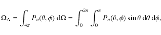
where
For most antennas, the normalized power pattern has considerably larger values for a certain range of both
7.1 LFI main beam characterisation
Far field radiation patterns were computed on the co- and cross-polar
basis according to Ludwig's third definition in UV-spherical grids. We
computed the main beam angular resolution of each feed model analysed,
as well as all major electromagnetic characteristics reported in
Tables 2
and 3.
U (
![]() )
and V (
)
and V (
![]() )
range from -0.026 to 0.026 (
)
range from -0.026 to 0.026 (
![]() )
for the 30 and 44 GHz channels, and from -0.015 to
0.015 (
)
for the 30 and 44 GHz channels, and from -0.015 to
0.015 (
![]() )
for the 70 GHz channel. Each grid has been sampled with
)
for the 70 GHz channel. Each grid has been sampled with ![]() points,
therefore
points,
therefore ![]() for the 30 and 44 GHz channels and 10-4
for the 70 GHz channel.
In Table 2,
the coordinate systems in which each main beam was computed are
reported:
for the 30 and 44 GHz channels and 10-4
for the 70 GHz channel.
In Table 2,
the coordinate systems in which each main beam was computed are
reported: ![]() and
and ![]() correspond to the centre of the UV-grids shown in this section. In
Table 3,
relevant main beam characteristics computed at the central frequency
are summarized, such as the full width half maximum, the cross polar
discrimination factor, and the main beam depolarization parameter.
In Fig. 9,
the contour plot in the UV-plane of the co- and cross-polar components
is shown for the main beam #27 and #28 (Y-polarized).
The lines in the contour plots, normalized with respect to the power
peak (the directivity reported in Table 3 for the
co-polar plot and the directivity minus the XPD for the cross- polar
plot), are at -3, -10, -20, -30, -40, -50, and -60. The colour scales
goes from -90 to 0 dB.
Figure 10
shows the differences between the two polarization X- and Y- for the
main beam #27, which are imperceptible below -40 dB.
In Figs. 11
and 12,
the contour plot in the UV-plane of the co- and cross-polar components
is shown for the main beam #24, #26, #21, #22, and #23
(Y-polarized), respectively.
correspond to the centre of the UV-grids shown in this section. In
Table 3,
relevant main beam characteristics computed at the central frequency
are summarized, such as the full width half maximum, the cross polar
discrimination factor, and the main beam depolarization parameter.
In Fig. 9,
the contour plot in the UV-plane of the co- and cross-polar components
is shown for the main beam #27 and #28 (Y-polarized).
The lines in the contour plots, normalized with respect to the power
peak (the directivity reported in Table 3 for the
co-polar plot and the directivity minus the XPD for the cross- polar
plot), are at -3, -10, -20, -30, -40, -50, and -60. The colour scales
goes from -90 to 0 dB.
Figure 10
shows the differences between the two polarization X- and Y- for the
main beam #27, which are imperceptible below -40 dB.
In Figs. 11
and 12,
the contour plot in the UV-plane of the co- and cross-polar components
is shown for the main beam #24, #26, #21, #22, and #23
(Y-polarized), respectively.
The cross-polar response of the OMT affects the beam pattern in a significant way below the -40 dB contour since the co-polar component is a linear combination of the co- and cross-polar pattern with coefficients of about 1 and 10-4. A detailed study of the LFI polarization capability is reported in Leahy et al. (2010).
![\begin{figure}
\par\begin{tabular}{c c}
\includegraphics[width=9pc,clip]{images/...
...cludegraphics[width=9pc,clip]{images/12891fg18.ps}\\
\end{tabular}
\end{figure}](/articles/aa/full_html/2010/12/aa12891-09/img78.png)
|
Figure 9:
Contour plot in the UV-plane (
-0.026 < U,V
< 0.026) of the main beam co-polar (left side)
and cross-polar (right side) component computed for
the 30 GHz feed horns #27 (first row)
and #28 (second row), assuming an ideal
telescope. The fit bivariate Gaussian contours are superimposed with
dotted lines and the resulting averaged FWHM is
32.58 |
| Open with DEXTER | |
| Figure 10: Contour plot in the UV-plane of the differences between the main beam #27 computed assuming the X-polarized feed and the main beam computed assuming the Y-polarized feed. The differences in the co- (left side) and cross- (right side) polar components are normalized to the local amplitude and expressed in dB. Table 3 quantitatively shows the differences between the two polarizations of the same feed. |
|
| Open with DEXTER | |
![\begin{figure}
\par\begin{tabular}{c c}
\includegraphics[width=9pc,clip]{images/...
...cludegraphics[width=9pc,clip]{images/12891fg24.ps}\\
\end{tabular}
\end{figure}](/articles/aa/full_html/2010/12/aa12891-09/img80.png)
|
Figure 11: Contour plot in the UV- plane ( -0.026 < U,V < 0.026) of the main beam co- (left side) and cross- (right side) polar components computed for the feed horns #24 (first row) and #26 (second row). The fit bivariate Gaussian contours are superimposed with dotted lines and the resulting averaged FWHM is 22.82 and 28.90, respectively. The lines in the contour plots represent levels of -3, -10, -20, -30, -40, -50, and -60. The colour scales go from -90 to 0 dB. |
| Open with DEXTER | |
![\begin{figure}
\par\begin{tabular}{c c}
\includegraphics[width=10pc,clip]{images...
...ludegraphics[width=10pc,clip]{images/12891fg30.ps}\\
\end{tabular}
\end{figure}](/articles/aa/full_html/2010/12/aa12891-09/img81.png)
|
Figure 12: Contour plot in the UV-plane ( -0.015 < U,V < 0.015) of the main beam co- (left side) and cross- (right side) polar components computed for the feed horns #21 (third row), #22 (fourth), and #23 (fifth row). The fit bivariate Gaussian contours are superimposed with dotted lines and the resulting averaged FWHM is 12.49, 12.71, and 13.05 arcmin, respectively. The lines in the contour plots represent levels of -3, -10, -20, -30, -40, -50, and -60. The colour scales go from -90 to 0 dB. |
| Open with DEXTER | |
8 LFI sidelobes
Power that does not originate in sources located in the main beam
direction (i.e, the straylight) enters detectors through the sidelobes
of the radiation pattern generating a signal that may be
indistinguishable from signals induced by CMB fluctuations in the main
beam.
More than the spurious signal itself, fluctuations in the straylight
signal contaminate the measurements mainly on large and intermediate
angular scales (i.e., at multipoles ![]() less than
less than ![]() 100),
and must be kept below a level of few
100),
and must be kept below a level of few ![]() K (the required straylight rejection levels must
be at about 10-9, 10-7,
and 10-6 for the Sun, Earth, and Galactic plane,
respectively). The control of this systematic effect was achieved by
accurate predictions of the LFI beams.
K (the required straylight rejection levels must
be at about 10-9, 10-7,
and 10-6 for the Sun, Earth, and Galactic plane,
respectively). The control of this systematic effect was achieved by
accurate predictions of the LFI beams.
In principle, Physical optics is the most accurate method for
predicting beams and may be used in all regions surrounding the
reflector antenna system. Neverthless, as the frequency increases the
reflectors need to be more precisely sampled.
In addition, a finer integration grid is required because in the
sidelobe region, the PO integrand becomes increasingly
oscillatory.
For a two-reflector antenna system such as Planck,
the computation time increases as the fourth power of the frequency,
and sidelobe simulations would be impractical for LFI.
Although a full PO computation would be required to predict accurately
the antenna pattern of the telescope, this is not feasible for the full
spacecraft simulations since the PO approach cannot be applied
correctly within a reasonable time when multiple diffractions and
reflections between scatterers are involved. For this reason, the
GRASP8 multi-reflector GTD (MrGTD) was used to compute 4![]() beam. MrGTD computes the scattered field from the reflectors performing
a backward ray tracing, and represents a suitable method for predicting
the full-sky radiation pattern of complex mm-wavelength optical systems
in which the computational time is frequency-independent.
beam. MrGTD computes the scattered field from the reflectors performing
a backward ray tracing, and represents a suitable method for predicting
the full-sky radiation pattern of complex mm-wavelength optical systems
in which the computational time is frequency-independent.
8.1 LFI sidelobe characterisation
![\begin{figure}
\par\begin{tabular}{c}
\includegraphics[width=11pc, angle=90,clip...
...hics[width=11pc, angle=90,clip]{images/12891fg32.ps}\end{tabular}\end{figure}](/articles/aa/full_html/2010/12/aa12891-09/img84.png)
|
Figure 13:
Co- (top panel) and cross- (bottom panel)
polar components of the 4 |
| Open with DEXTER | |
To first approximation, the efficiency of an optical system in
rejecting external straylight contamination is quantified by the
fractional amount of power entering far from the main beam in the case
of an isotropic signal.
We provide here this information for all LFI beams in terms of relative
(percent) contributions from the intermediate and far beam to the beam ![]() integral.
The intermediate beam includes here the region at angles
between
integral.
The intermediate beam includes here the region at angles
between ![]() (
(![]() ,
,
![]() ,
respectively) and
,
respectively) and ![]() from the beam centre for the beams at 70 (resp. 44,
30) GHz, while the far beam includes the regions at angles
greater than
from the beam centre for the beams at 70 (resp. 44,
30) GHz, while the far beam includes the regions at angles
greater than ![]() from the beam centre.
The main, intermediate, and far beams are known in tabulated form and
with different resolutions. Thus, the accuracy in the computations of
their integrals cannot be extremely high. We exploited three different
numerical methods and compared the corresponding results: (i)
a 2D quadrature in
from the beam centre.
The main, intermediate, and far beams are known in tabulated form and
with different resolutions. Thus, the accuracy in the computations of
their integrals cannot be extremely high. We exploited three different
numerical methods and compared the corresponding results: (i)
a 2D quadrature in ![]() and
and ![]() ,
performed with the routine D01DAF of the Mark 21 version of
the NAG numerical library; (ii) a combination of two
1D quadratures, a Gaussian quadrature (adapted in double precision and
with 2048 grid points) from Press et al. (1992) for the
integral in
,
performed with the routine D01DAF of the Mark 21 version of
the NAG numerical library; (ii) a combination of two
1D quadratures, a Gaussian quadrature (adapted in double precision and
with 2048 grid points) from Press et al. (1992) for the
integral in ![]() and the NAG routine D01AJF for the (more difficult) integral
in
and the NAG routine D01AJF for the (more difficult) integral
in ![]() ;
(iii) a summation over the relevant pixels of the
beam responses projected into a map at
;
(iii) a summation over the relevant pixels of the
beam responses projected into a map at ![]() or 1024 in the HEALPix
or 1024 in the HEALPix![]() scheme (Gorski et al. 2005)
for the far beam or for the intermediate and main beam, respectively. A
robust bilinear interpolation is adopted to estimate the beam response
between tabulated points. Methods (ii) and (iii)
give consistent (i.e., with relative differences always less
than 0.08%) results for the far beams and we report here their
average (while method (i) provides only a
rough estimate, in agreement with the others only within a factor of
scheme (Gorski et al. 2005)
for the far beam or for the intermediate and main beam, respectively. A
robust bilinear interpolation is adopted to estimate the beam response
between tabulated points. Methods (ii) and (iii)
give consistent (i.e., with relative differences always less
than 0.08%) results for the far beams and we report here their
average (while method (i) provides only a
rough estimate, in agreement with the others only within a factor of ![]() 2, because
of its relatively poorer sampling of the 2D function).
All methods give very consistent results for the main beams (agreement
level always superior to 0.04% for methods (i)
and (ii) and better than 2.3% for
methods (i) - or (ii) - and (iii)).
For the intermediate beams, the level of agreement between the results
obtained with the three methods depends significantly on the beam
considered and ranges from 0.1% to 15%, being on
average several percent.
We report here the results based on method (ii),
which samples the 2D function more effectively and allows good
control of integration accuracy.
Obviously, the true accuracy depends on the beam sampling
2, because
of its relatively poorer sampling of the 2D function).
All methods give very consistent results for the main beams (agreement
level always superior to 0.04% for methods (i)
and (ii) and better than 2.3% for
methods (i) - or (ii) - and (iii)).
For the intermediate beams, the level of agreement between the results
obtained with the three methods depends significantly on the beam
considered and ranges from 0.1% to 15%, being on
average several percent.
We report here the results based on method (ii),
which samples the 2D function more effectively and allows good
control of integration accuracy.
Obviously, the true accuracy depends on the beam sampling
The results are summarized in Table 4, where we also
provide predictions for the Galactic straylight contamination.
For each (normalized to the maximum power measured in the field, i.e.,
the main beam power peak) LFI FM beam (Cols. 1 and 2)
we report: the ![]() integral as the sum (the global integral GI,
Col. 3) of the contributions from the main, intermediate, and
far beam and the relative (percent) contributions to it from the
intermediate ( IB, Col. 4) and far
( FB, Col. 7) beam. The transition
between intermediate and far beam was adopted here at
integral as the sum (the global integral GI,
Col. 3) of the contributions from the main, intermediate, and
far beam and the relative (percent) contributions to it from the
intermediate ( IB, Col. 4) and far
( FB, Col. 7) beam. The transition
between intermediate and far beam was adopted here at ![]() ,
,
![]() ,
and
,
and ![]() from the beam centre, respectively, at 70 GHz,
44 GHz, and 30 GHz. Columns 5 and 6
(respectively, 8 and 9) report the Galactic straylight
contamination ( GSC, in
from the beam centre, respectively, at 70 GHz,
44 GHz, and 30 GHz. Columns 5 and 6
(respectively, 8 and 9) report the Galactic straylight
contamination ( GSC, in ![]() K RMS
and peak-to-peak antenna temperature) evaluated considering the
intermediate (respectively, far) pattern region. The RMS
and peak-to-peak values reported in the table were estimated by a
proper rescaling of the results presented in Burigana et al. (2004)
considering the fractional contributions to the
K RMS
and peak-to-peak antenna temperature) evaluated considering the
intermediate (respectively, far) pattern region. The RMS
and peak-to-peak values reported in the table were estimated by a
proper rescaling of the results presented in Burigana et al. (2004)
considering the fractional contributions to the ![]() integrated antenna pattern from intermediate and far beams and the
frequency behaviour of the considered foreground components (diffuse
dust, free-free, and synchrotron emission, and HII regions).
integrated antenna pattern from intermediate and far beams and the
frequency behaviour of the considered foreground components (diffuse
dust, free-free, and synchrotron emission, and HII regions).
In principle, the straylight contamination from the CMB dipole
is important only for the even multipoles, where it is expected to
dominate over the
Galactic one at frequencies greater or equal to 44 GHz (Burigana
et al. 2006).
Given the fractional contributions from the far sidelobes to
the ![]() integrated antenna pattern reported in Table 4, we expect that
dipole straylight
will not significantly affect the recovery of the angular power
spectrum at low multipoles and the analysis of large-scale anomalies
(Gruppuso et al. 2007),
provided that the relative uncertainty in the modelling of the far
sidelobes is
integrated antenna pattern reported in Table 4, we expect that
dipole straylight
will not significantly affect the recovery of the angular power
spectrum at low multipoles and the analysis of large-scale anomalies
(Gruppuso et al. 2007),
provided that the relative uncertainty in the modelling of the far
sidelobes is ![]() 20%.
20%.
Table 4: Galactic straylight contamination.
![\begin{figure}
\par\begin{tabular}{c}
\includegraphics[width=11pc, angle=90,clip...
...hics[width=11pc, angle=90,clip]{images/12891fg34.ps}\end{tabular}\end{figure}](/articles/aa/full_html/2010/12/aa12891-09/img93.png)
|
Figure 14:
Co- (top panel) and cross- (bottom panel)
polar components of the 4 |
| Open with DEXTER | |
![\begin{figure}
\par\begin{tabular}{c}
\includegraphics[width=11pc, angle=90,clip...
...hics[width=11pc, angle=90,clip]{images/12891fg36.ps}\end{tabular}\end{figure}](/articles/aa/full_html/2010/12/aa12891-09/img94.png)
|
Figure 15:
Co- (top panel) and cross- (bottom panel)
polar components of the 4 |
| Open with DEXTER | |
9 Conclusions
From the beginning of the Phase A study to the current flight
configuration, we have reported reported the history of the
optimization of the LFI optical interface. The definition,
optimization, and characterization of the LFI feed horns coupled the Planck
telescope have been derived by means of electromagnetic simulations
devoted to maximizing the angular resolution and at the same time
minimizing systematic effects produced by the sidelobes of the
radiation pattern. The position and orientation of each horn was set
taking into account the mechanical constraints imposed by the LFI
interfaces and the 4 K reference loads. The feeds and
corresponding OMTs have been adjusted in the focal surface in such a
way that the main beam polarization directions of the two symmetrically
located feed horns in the FPU are at an angle of 45 degrees
when they observe the same direction in the sky, in order to measure
the Q and U Stokes parameters and thus the linear
polarization of the CMB. Finally, the LFI optical performance computed
with the ideal telescope has been presented. The requirements have been
met and in some cases exceeded. Typical LFI main beams have angular
resolutions of about 33![]() ,
24
,
24![]() ,
and 13
,
and 13![]() ,
respectively, at 30 GHz, 44 GHz, and 70 GHz,
slightly exceeding the requirements for the cosmological
70 GHz channel. The beams have been delivered to the LFI data
processing center and they are the current baseline data used in the
testing of the data reduction pipeline.
Of course, the performance in-flight will be different owing to the
true telescope and focal surface alignment, the surface roughness, and
the distortion of the reflectors caused by the cooldown. However,
simulations on the Planck radio frequency flight
model (Tauber et al. 2010) have shown that the LFI performance
is quite similar to the ideal case, so values reported in the tables of
this paper (beam characteristics and straylight contamination) are
presumably not far from the true values.
,
respectively, at 30 GHz, 44 GHz, and 70 GHz,
slightly exceeding the requirements for the cosmological
70 GHz channel. The beams have been delivered to the LFI data
processing center and they are the current baseline data used in the
testing of the data reduction pipeline.
Of course, the performance in-flight will be different owing to the
true telescope and focal surface alignment, the surface roughness, and
the distortion of the reflectors caused by the cooldown. However,
simulations on the Planck radio frequency flight
model (Tauber et al. 2010) have shown that the LFI performance
is quite similar to the ideal case, so values reported in the tables of
this paper (beam characteristics and straylight contamination) are
presumably not far from the true values.
Planck is a project of the European Space Agency with instruments funded by ESA member states, and with special contributions from Denmark and NASA (USA). The Planck-LFI project is developed by an International Consortium lead by Italy and involving Canada, Finland, Germany, Norway, Spain, Switzerland, UK, USA. The Italian contribution to Planck is supported by the Italian Space Agency (ASI). We wish to thank people of the Herschel/Planck Project of ESA, ASI, THALES Alenia Space Industries, and the LFI Consortium that are involved in activities related to optical simulations. Some of the results in this paper have been derived using the HEALPix (Górski, Hivon, and Wandelt 1999). Special thanks to Denis Dubruel (THALES Alenia Space), for his professional collaboration in all these years. We warmly thank David Pearson for constructive comments and suggestions, and for the careful reading of the first version of this work.
Appendix A: Main beam descriptive parameters
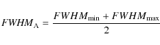
Owing to the telescope configuration and the feed horn off-axis location on the focal surface, the main beams are strongly distorted and their shape differs from a Gaussian. In other words, the main beams cannot be mathematically represented by a single parameter (for instance, the full width half maximum) and by a simple formula (Gaussian function, polynomial function) because aberrations prevail at power levels lower than -10 dB. However, it is indispensable to characterize the main beams as precisely as possible, and several descriptive parameters have been evaluated: the angular resolution (FWHM), the ellipticity (e), the main beam directivity (A.1 Angular resolution
For CMB anisotropy measurements, an effective angular resolution can be defined as the FWHM of a perfect (symmetric Gaussian) beam, which produces the same signal as the distorted beam when the CMB field is observed (Burigana et al. 1998). Nevertheless, this definition involves astrophysical simulations taking into account the scanning strategy and the CMB expected anisotropy map (or the WMAP results). Owing to the large computation time, this approach is not practical for the optimization activity of the LFI feed horns.Main beam aberrations degrade its angular resolution. Instead of the effective FWHM, the angular resolution can be evaluated by taking the average FWHM of the distorted beam. The average FWHM has been computed in three different ways, using the minimum and maximum values:
- arithmetic average: by taking the average value between the
maximum and minimum of the FWHM of the distorted
beam:
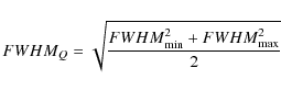
- quadratic average:
by taking the quadratic mean between the maximum and minimum of the FWHM
of the distorted beam:
- equal area average
![[*]](/icons/foot_motif.png) :
the distorted beam exhibits the same beam area of a symmetric beam with
a FWHM defined as:
:
the distorted beam exhibits the same beam area of a symmetric beam with
a FWHM defined as:
|
|||
![$\displaystyle \qquad-\left[ \frac{1}{2} \cdot {{\it FWHM}}_{\rm min} \cdot \left( 1 + e - \sqrt{e} - \frac{\sqrt{2}}{2} \sqrt{1+e^2} \right) \right]$](/articles/aa/full_html/2010/12/aa12891-09/img102.png)
|
(A.1) |
or alternatively:
|
|
|||
![$\displaystyle \quad -\left[ \frac{1}{2} \cdot {{\it FWHM}}_{\rm max} \cdot \lef...
...t{\frac{1}{e}} - \frac{\sqrt{2}}{2} \sqrt{1+\frac{1}{e^2}} \right) \right]\cdot$](/articles/aa/full_html/2010/12/aa12891-09/img103.png)
|
(A.2) |
The term between the inner brackets is small (![]() 10-4-10-5),
and it is zero in the case of perfect symmetric beam (e
= 1). Although it is important to include in the data analysis the
detailed information of the beam shape, these small differences are not
a concern for the angular resolution requirements, and the adopted
angular resolution is the FWHM computed
arithmetically (FWHM
10-4-10-5),
and it is zero in the case of perfect symmetric beam (e
= 1). Although it is important to include in the data analysis the
detailed information of the beam shape, these small differences are not
a concern for the angular resolution requirements, and the adopted
angular resolution is the FWHM computed
arithmetically (FWHM![]() ).
).
A.2 Directivity and gain
Directivity is the ability of an antenna to focus energy in a
particular direction when transmitting, or when receiving to receive
energy preferentially from a particular direction. In a realistic, but
lossless antenna (i.e., of efficiency ![]() ), the
directivity D
), the
directivity D
![]() is essentially equal to the gain G
is essentially equal to the gain G
![]() :
:
Thus, gain or directivity is also a normalized power pattern similar to Pn in Eq. (3) with the difference that the normalizing factor is
|
(A.4) |
where
|
(A.5) |
and
A.3 Cross polar discrimination factor
The cross polar discrimination factor (XPD, usually expressed in dB) was computed as the ratio of the directivity to the co- and cross-polar components
|
(A.6) |
A.4 Depolarization parameter
The depolarization parameter (d) was obtained by
computing the Stokes parameters in each point of the regular UV- grid:
| SI(u,v) | = | (A.7) | |
| SQ(u,v) | = | (A.8) | |
| SU(u,v) | = | (A.9) | |
| SV(u,v) | = | (A.10) |
in which
| (A.11) |
and, finally
|
(A.12) |
A.5 Rotation angle
The rotation angle of the polarization ellipse (![]() ,
ranges from -90
,
ranges from -90![]() to 90
to 90![]() )
is computed as
)
is computed as
|
(A.13) |
In Fig. A.1, the rotation angles of the 70 GHz main beam #21 and the 44 GHz main beam #24 (both X-polarized) are shown and it should be noted that the main beam is mainly linear polarized close to the main beam pointing direction, as discussed in Sect. 5.
| Figure A.1: Polarization angle of the main beam #21 at 70 GHz (left side) and main beam #24 at 44 GHz (right side). |
|
| Open with DEXTER | |
A.6 Spillover
By means of simple ray-tracing, the main beam spillover (which points towards the Galactic plane) can be evaluated quickly for each feed model, taking into account the radiation pattern of the feed and the geometry of the optical system. This is a first approximation to the true spillover since it takes into account only the rays reflected by the subreflector that do not hit the main reflector.A more precise but time-consuming computation of the spillover
was performed using physical optics and the results are very similar.
With PO, the spillover was computed as 1 - W,
where W is the relative power hitting the
main reflector.
The power contained in the incident field on the main reflector is
computed by integrating Poynting's vector P
over the surface:
|
(A.14) |
where Re denotes the real part and * the complex conjugate. The power
|
(A.15) |
where
|
(A.16) |
which is a surface integral with the integration variable
References
- Bersanelli, M., Mandolesi, N., Butler, R. C., et al. 2010, A&A, 520, A4 [NASA ADS] [CrossRef] [EDP Sciences] [Google Scholar]
- Burigana, C., Maino, D., Mandolesi, N., et al. 1998, A&AS., 130, 551 [Google Scholar]
- Burigana, C., Maino, D., Górski, K. M., et al. 2001, A&A, 373, 345 [NASA ADS] [CrossRef] [EDP Sciences] [Google Scholar]
- Burigana, C., Sandri, M., Villa, F., et al. 2004, A&A, 428, 311 [NASA ADS] [CrossRef] [EDP Sciences] [Google Scholar]
- Burigana, C., Gruppuso, A., & Finelli, F. 2006, MNRAS, 371, 1570 [NASA ADS] [CrossRef] [Google Scholar]
- Clarricoats, P. J. B., & Olver, A. D. 1984, Corrugated horns for microwave antennas, IEE, London [Google Scholar]
- D'Arcangelo, O., Figini, L., Simonetto, A., et al. 2010, JINST, 4, T12007 [Google Scholar]
- Dubruel, D., Cornut, M., Fargant, et al. 2000, ESA Conf. Proc. SP-444, ed. D. Danesy, & H. Sawaya, CD-ROM [Google Scholar]
- Dupac, X. Baseline observation strategy definition document, Planck/PSO/2006-030, Rev 2 [Google Scholar]
- Górski, K. M., Hivon, E., Banday, A. J., et al. 2005, ApJ, 622, 759 [NASA ADS] [CrossRef] [Google Scholar]
- Gruppuso, A., Burigana, C., & Finelli, F. 2007, MNRAS, 376, 907 [NASA ADS] [CrossRef] [Google Scholar]
- Lamarre, J.-M., Puget, J.-L., Ade, P. A. R., et al. 2010, A&A, 520, A9 [NASA ADS] [CrossRef] [EDP Sciences] [Google Scholar]
- Leahy, J. P., Bersanelli, M., D'Arcangelo, O., et al. 2010, A&A, 520, A8 [NASA ADS] [CrossRef] [EDP Sciences] [Google Scholar]
- Ludwig, A. C. 1973, The Definition of Cross Polarization, IEEE Transactions on Antennas and Propagation, 116 [Google Scholar]
- Maino, D., Burigana, C., Górski, K. M., Mandolesi, N., & Bersanelli, M. 2002, A&A, 387, 356 [NASA ADS] [CrossRef] [EDP Sciences] [Google Scholar]
- Mandolesi, N., Bersanelli, M., Butler, R. C., et al. 2010, A&A, 520, A3 [Google Scholar]
- Nielsen, P. H., RF Effect of Core Print-through Distortion on the Planck Telescope, PL-COM-DRI-AN-MIR012 [Google Scholar]
- Olver, A. D., & Xiang, J. 1988, IEEE Trans. On Antenna Propagation, 36, 936 [NASA ADS] [CrossRef] [Google Scholar]
- Pontoppidan, K. 1999, Technical Description of GRASP8, TICRA [Google Scholar]
- Press, W. H., Flannery, B. P., Teukolski, S. A., & Vetterling, W. T. 1992, Numerical Recipes (Cambridge University Press) [Google Scholar]
- Sandri, M., & Villa, F 2002, Int. Rep. INAF-IASFBO/342/2002, May [Google Scholar]
- Sandri, M., Villa, F., Bersanelli, M., et al. 2002, 25th ESA Antenna Workshop on Satellite Antenna Technology ESA Conf. Proc. WPP-202, 621 [Google Scholar]
- Sandri, M., Villa, F., Burigana, C., et al. 2004, A&A, 428, 299 [NASA ADS] [CrossRef] [EDP Sciences] [Google Scholar]
- Tauber J. A., Norgaard-Nielsen H. U., Ade, P. A. R., et al. 2010, A&A, 520, A2 [NASA ADS] [CrossRef] [EDP Sciences] [Google Scholar]
- Villa, F., Bersanelli, M., Burigana, C., et al. 2002, AIP Conf. proc. 616, ed. M. De Petris, & M. Gervasi, 224 [NASA ADS] [CrossRef] [Google Scholar]
- Villa, F., Terenzi, L., Sandri, M., et al. 2010, A&A, 520, A6 [NASA ADS] [CrossRef] [EDP Sciences] [Google Scholar]
- Wilson, R. N. 1996, Reflecting Telescope Optics I, Springer Astron. Astrophys. Library [Google Scholar]
Footnotes
- ...Planck
- Planck (http://www.esa.int/Planck) is an ESA project with instruments provided by two scientific Consortia funded by ESA member states (in particular the lead countries: France and Italy) with contributions from NASA (USA), and telescope reflectors provided in a collaboration between ESA and a scientific Consortium led and funded by Denmark.
- ... contractor
- Thales Alenia Space - France, formerly Alcatel Space.
- ... GRASP8
- The GRASP software was developed by TICRA (Copenhagen, DK) for analysing general reflector antennas.
- ... HEALPix
- http://healpix.jpl.nasa.gov
- ... average
- The meaning of equal area is derived from Maino
et al. (2002).
For Gaussian elliptical beams, FWHM
 = FWHME.
All Tables
Table 1: Location and orientation of the LFI feed horns.
Table 2: Main beam frames.
Table 3: Main beam characteristics at the central frequency.
Table 4: Galactic straylight contamination.
All Figures
|
|
Figure 1:
Lateral and top view of the telescope unit consisting of the reflectors
and the support structure; the hexagonal support structure is readily
seen as well as the field of view (in gray) (left panel).
The telescope unit allocated into Planck satellite (right
panel). The vertical axis is the spin axis of the satellite
and the line of sight is tilted by |
| Open with DEXTER | |
| In the text | |
|
|
Figure 2: A CAD model of the Planck focal plane, which is located directly below the telescope primary mirror. It comprises the HFI bolometric detector array (small feed horns on golden circular base) and the LFI radio receiver array (larger feed horns around the HFI). The box holding the feedhorns appears to be transparent in this view, to also show the elements inside and behind it ( top panel). The HFI and LFI feed horns are seen reflected in the primary mirror of the Planck telescope in the clean room at Kourou, French Guiana ( bottom panel). © ESA/Thales. |
| Open with DEXTER | |
| In the text | |
|
|
Figure 3: Simulated co-polar pattern, in the E- plane, of the FM feed horns at 70 (FH21, FH22, and FH23), 44 (FH24 and FH25), and 30 (FH27) GHz assuming the designed profile. |
| Open with DEXTER | |
| In the text | |
| |
Figure 4: 10 dB contour of all horn patterns on the sub (left panel) and main (right panel) reflectors: the contours corresponding to the 30 GHz patterns are pink, the 44 GHz contours are blue, and those at 70 GHz are green. |
| Open with DEXTER | |
| In the text | |
|
|
Figure 5:
Field distribution on Planck mirrors (the
sub-reflector is on the left and the main reflector is on the right)
for a 70 GHz feed horn assuming a Gaussian feed approximation
(
|
| Open with DEXTER | |
| In the text | |
| |
Figure 6:
Difference in the field distribution on the Planck
mirrors between computations with the flight model feed and the
Gaussian approximation. Differences data are in percent ((
|
| Open with DEXTER | |
| In the text | |
|
|
Figure 7: Edge-taper curve on the primary mirror computed assuming a Gaussian illumination (red curve) and a realistic illumination (blue curve). The nominal edge-taper of the two feeds is the same: 17 dB at 22 degrees. |
| Open with DEXTER | |
| In the text | |
|
|
Figure 8: Footprint of the LFI focalplane on the sky as seen by an observer looking towards the satellite along its optical axis. The origin of a right-handed uv-coordinate system is at the center of the focalplane (LOS). The z-axis is along the line-of-sight and points towards the observer. Labels from 18 to 23 refer to 70 GHz horns, from 24 to 26 refer to 44 GHz horns, and 27 and 28 refer to 30 GHz horns. Each beam has its own coordinate system as shown in the figure. The focalplane scans the sky as the satellite spins. The scanning direction is indicated by an arrow. The +u axis points to the spin axis of the satellite. The centers of the 30 GHz beams sweep about 1 degree from the ecliptic poles when the spin axis is in the ecliptic plane. |
| Open with DEXTER | |
| In the text | |
|
|
Figure 9:
Contour plot in the UV-plane (
-0.026 < U,V
< 0.026) of the main beam co-polar (left side)
and cross-polar (right side) component computed for
the 30 GHz feed horns #27 (first row)
and #28 (second row), assuming an ideal
telescope. The fit bivariate Gaussian contours are superimposed with
dotted lines and the resulting averaged FWHM is
32.58 |
| Open with DEXTER | |
| In the text | |
| |
Figure 10: Contour plot in the UV-plane of the differences between the main beam #27 computed assuming the X-polarized feed and the main beam computed assuming the Y-polarized feed. The differences in the co- (left side) and cross- (right side) polar components are normalized to the local amplitude and expressed in dB. Table 3 quantitatively shows the differences between the two polarizations of the same feed. |
| Open with DEXTER | |
| In the text | |
|
|
Figure 11: Contour plot in the UV- plane ( -0.026 < U,V < 0.026) of the main beam co- (left side) and cross- (right side) polar components computed for the feed horns #24 (first row) and #26 (second row). The fit bivariate Gaussian contours are superimposed with dotted lines and the resulting averaged FWHM is 22.82 and 28.90, respectively. The lines in the contour plots represent levels of -3, -10, -20, -30, -40, -50, and -60. The colour scales go from -90 to 0 dB. |
| Open with DEXTER | |
| In the text | |
|
|
Figure 12: Contour plot in the UV-plane ( -0.015 < U,V < 0.015) of the main beam co- (left side) and cross- (right side) polar components computed for the feed horns #21 (third row), #22 (fourth), and #23 (fifth row). The fit bivariate Gaussian contours are superimposed with dotted lines and the resulting averaged FWHM is 12.49, 12.71, and 13.05 arcmin, respectively. The lines in the contour plots represent levels of -3, -10, -20, -30, -40, -50, and -60. The colour scales go from -90 to 0 dB. |
| Open with DEXTER | |
| In the text | |
|
|
Figure 13:
Co- (top panel) and cross- (bottom panel)
polar components of the 4 |
| Open with DEXTER | |
| In the text | |
|
|
Figure 14:
Co- (top panel) and cross- (bottom panel)
polar components of the 4 |
| Open with DEXTER | |
| In the text | |
|
|
Figure 15:
Co- (top panel) and cross- (bottom panel)
polar components of the 4 |
| Open with DEXTER | |
| In the text | |
| |
Figure A.1: Polarization angle of the main beam #21 at 70 GHz (left side) and main beam #24 at 44 GHz (right side). |
| Open with DEXTER | |
| In the text | |
Copyright ESO 2010
Current usage metrics show cumulative count of Article Views (full-text article views including HTML views, PDF and ePub downloads, according to the available data) and Abstracts Views on Vision4Press platform.
Data correspond to usage on the plateform after 2015. The current usage metrics is available 48-96 hours after online publication and is updated daily on week days.
Initial download of the metrics may take a while.