| Issue |
A&A
Volume 519, September 2010
|
|
|---|---|---|
| Article Number | A89 | |
| Number of page(s) | 9 | |
| Section | Cosmology (including clusters of galaxies) | |
| DOI | https://doi.org/10.1051/0004-6361/201014058 | |
| Published online | 16 September 2010 | |
Impact of supernova feedback on the Tully-Fisher relation
M. E. De Rossi1,2 - P. B. Tissera1,2 - S. E. Pedrosa1,2
1 - Consejo Nacional de Investigaciones Científicas y Técnicas, CONICET, Argentina
2 - Instituto de Astronomía y Física del Espacio, Casilla de Correos 67, Suc. 28, 1428 Buenos Aires, Argentina
Received 13 January 2010 / Accepted 27 May 2010
Abstract
Context. Recent observational results have found a bend in
the Tully-Fisher relation in such a way that low-mass systems lie below
the linear relation described by more massive galaxies.
Aims. We intend to investigate the origin of the observed
features in the stellar and baryonic Tully-Fisher relations and analyse
the role played by galactic outflows on their determination.
Methods. Cosmological hydrodynamical simulations which include
supernova feedback were performed in order to follow the dynamical
evolution of galaxies.
Results. We found that supernova feedback is a fundamental
process for reproducing the observed trends in the stellar Tully-Fisher
relation. Simulated slowly rotating systems tend to have lower stellar
masses than those predicted by the linear fit to the massive end of the
relation, consistently with observations. This feature is not present
if supernova feedback is turned off. In the case of the baryonic
Tully-Fisher relation, we also detect a weaker tendency for smaller
systems to lie below the linear relation described by larger ones. This
behaviour arises as a result of the more efficient action of supernovae
in the regulation of the star formation process and in the triggering
of powerful galactic outflows in shallower potential wells, which may
heat up and/or expel part of the gas reservoir.
Key words: galaxy: formation - galaxy: evolution - galaxy: structure
1 Introduction
The origin of the Tully-Fisher relation (Tully & Fisher 1977) has been analysed by numerous
observational and theoretical works since it provides important constraints on
galaxy formation models (e.g. Avila-Reese et al. 1998; Mo et al. 1998; Avila-Reese et al. 2008).
Originally defined as the relation between the luminosity and the rotation velocity
for spiral galaxies, it is now accepted that this is a proxy for the more fundamental
relation between stellar mass
and rotation velocity (e.g. Flores et al. 2006; Conselice et al. 2005; Cresci et al. 2009)
or even between baryonic mass and rotation velocity
(e.g. Puech et al. 2010; McGaugh 2005; Verheijen 2001; Gurovich et al. 2004; Bell & de Jong 2001) of the form
![]() .
Observational evidence suggests there is a break in the stellar Tully-Fisher relation (sTFR) at
a rotation velocity of
.
Observational evidence suggests there is a break in the stellar Tully-Fisher relation (sTFR) at
a rotation velocity of ![]()
![]() (McGaugh et al. 2000; Amorín et al. 2009).
Even more, recently McGaugh et al. (2010) have also reported a break in the baryonic Tully-Fisher relation (bTFR) but at a lower
velocity.
(McGaugh et al. 2000; Amorín et al. 2009).
Even more, recently McGaugh et al. (2010) have also reported a break in the baryonic Tully-Fisher relation (bTFR) but at a lower
velocity.
Assuming that galaxies formed in virialized haloes and that the percentage of gas transformed into stars
is independent of halo mass, a relation between stellar mass and circular velocity with a slope of
![]() is directly obtained (Mo et al. 1998; White & Frenk 1991).
This theoretical prediction is reproduced in cosmological simulations when ineffective mechanisms
to regulate the gas cooling and star
formation activity are introduced (Steinmetz & Navarro 1999; Tissera et al. 1997).
Therefore, changes in the slope of this relation to match observed reported values, which are on average
close to
is directly obtained (Mo et al. 1998; White & Frenk 1991).
This theoretical prediction is reproduced in cosmological simulations when ineffective mechanisms
to regulate the gas cooling and star
formation activity are introduced (Steinmetz & Navarro 1999; Tissera et al. 1997).
Therefore, changes in the slope of this relation to match observed reported values, which are on average
close to
![]() ,
might require the action
of other physical processes.
Theoretical findings suggest that the triggering of powerful mass-loaded galactic
winds by massive supernova (SN) explosions would have
an efficiency that depends on the virial halo so that stronger effects are expected in
low-mass systems
(Larson 1974). In fact, Dekel & Silk (1986) estimated analytically that
haloes with circular velocity lower than
,
might require the action
of other physical processes.
Theoretical findings suggest that the triggering of powerful mass-loaded galactic
winds by massive supernova (SN) explosions would have
an efficiency that depends on the virial halo so that stronger effects are expected in
low-mass systems
(Larson 1974). In fact, Dekel & Silk (1986) estimated analytically that
haloes with circular velocity lower than ![]() 100 km s-1 would be strongly affected by massive SN events.
Nonetheless, the role of galactic outflows on the origin of the relations between the stellar
and dynamical properties of dwarf
galaxies still constitutes an open problem (Mac Low & Ferrara 1999; Tassis et al. 2008).
In a cosmological framework, only recently has it been possible to start simulating the triggering of galactic
outflows on more physical basis (e.g. Scannapieco et al. 2006; Stinson et al. 2007; Governato et al. 2010).
In fact, cosmological simulations that include this process obtained sTFRs in more qualitative agreement with observations (Governato et al. 2007; Croft et al. 2009).
There is evidence
that the implementation of a suitable feedback model could account for a bend in the TFR as suggested by
semi-analytical works
(e.g. Dutton & van den Bosch 2009; Guo et al. 2010; Nagashima et al. 2005; Kang et al. 2005) and some hydrodynamical simulations
(e.g. Tassis et al. 2008).
However, a detailed analysis of the effects of SN feedback on the TFR using
a physically motivated model was still missing.
100 km s-1 would be strongly affected by massive SN events.
Nonetheless, the role of galactic outflows on the origin of the relations between the stellar
and dynamical properties of dwarf
galaxies still constitutes an open problem (Mac Low & Ferrara 1999; Tassis et al. 2008).
In a cosmological framework, only recently has it been possible to start simulating the triggering of galactic
outflows on more physical basis (e.g. Scannapieco et al. 2006; Stinson et al. 2007; Governato et al. 2010).
In fact, cosmological simulations that include this process obtained sTFRs in more qualitative agreement with observations (Governato et al. 2007; Croft et al. 2009).
There is evidence
that the implementation of a suitable feedback model could account for a bend in the TFR as suggested by
semi-analytical works
(e.g. Dutton & van den Bosch 2009; Guo et al. 2010; Nagashima et al. 2005; Kang et al. 2005) and some hydrodynamical simulations
(e.g. Tassis et al. 2008).
However, a detailed analysis of the effects of SN feedback on the TFR using
a physically motivated model was still missing.
In this paper, we present results on the analysis of the sTFR and bTFR by using a SN feedback model especially suitable to studying the formation of galaxies in cosmological scenarios (Scannapieco et al. 2006,2005), since it does not include any scale-dependent parameter and it is capable to produce the expected anti-correlation between the strength of the galactic outflows and the potential well of the haloes, as shown by Scannapieco et al. (2006).
This paper is organized as follows. Section 2 describes the numerical experiments. Section 3 outlines the results. In Sect. 4 we discuss about our main findings, and in Sect. 5 we present the conclusions of this work.
2 Numerical experiments
We performed cosmological simulations of a typical field region of the Universe
consistent with the concordance model. We adopt the following cosmological parameters:
![]() ,
,
![]() ,
,
![]() ,
a normalization of the power
spectrum of
,
a normalization of the power
spectrum of
![]() and
and
![]() ,
with h=0.7.
Two of the simulations were run with
,
with h=0.7.
Two of the simulations were run with
![]() (S230) particles, while a third one and a fourth one used
(S230) particles, while a third one and a fourth one used
![]() (S320) and
(S320) and
![]() (S160) to check numerical
effects.
In all cases, the simulated volumes correspond to a cubic box of a comoving
10 Mpc h-1 side length.
The particle masses for the dark and initial gas components are given
in Table 1.
Simulation S320 could only reach
(S160) to check numerical
effects.
In all cases, the simulated volumes correspond to a cubic box of a comoving
10 Mpc h-1 side length.
The particle masses for the dark and initial gas components are given
in Table 1.
Simulation S320 could only reach
![]() due to high computational costs.
By analysing the sTFR and bTFR in S230, S320, and S160, we check our results for numerical effects.
due to high computational costs.
By analysing the sTFR and bTFR in S230, S320, and S160, we check our results for numerical effects.
Table 1: Cosmological hydrodynamical simulations studied in this paper.
The simulations were performed by using a version of GADGET-3, an update of GADGET-2 optimized for massively parallel simulations of highly inhomogeneous systems (Springel 2005; Springel & Hernquist 2003). This version of GADGET-3 includes the multiphase model for the interstellar medium (ISM) and the SN feedback scheme of Scannapieco et al. (2006,2005). We ran the same initial condition with (S230) and without SN feedback (S230NF) in order to quantify the effects of SN-induced galactic winds.
The SN feedback scheme adopted in this work considers both type II
and type Ia SNe for the chemical and energy production. We adopt
![]() erg per SN event.
The chemical evolution model used in this code is the one developed by Mosconi et al. (2001) and, later on,
adapted by Scannapieco et al. (2005) for GADGET-2.
This model assumes the instantaneous recycling approximation (IRA) for SNII
erg per SN event.
The chemical evolution model used in this code is the one developed by Mosconi et al. (2001) and, later on,
adapted by Scannapieco et al. (2005) for GADGET-2.
This model assumes the instantaneous recycling approximation (IRA) for SNII![]() .
Lifetimes for the progenitors of
SNIa are randomly selected in the range
[108, 109] yr. The chemical yields for SNII are given by Woosley & Weaver (1995),
while those of SNIa correspond to the W7 model of Thielemann et al. (1993).
.
Lifetimes for the progenitors of
SNIa are randomly selected in the range
[108, 109] yr. The chemical yields for SNII are given by Woosley & Weaver (1995),
while those of SNIa correspond to the W7 model of Thielemann et al. (1993).
The SN feedback model is grafted onto a multiphase model especially designed to improve the description of the ISM,
allowing the coexistence of diffuse and dense gas phases. Within this new framework, the injection of energy and heavy
elements into different components of the ISM can be more realistically treated, leading to a more effective production
of galactic winds. The ejected energy is distributed into and managed differently by the so-called cold (temperature
![]() where
where
![]() K and density
K and density
![]() where
where
![]() is
is
![]() )
and hot (otherwise) ISM components. The hot phase thermalizes instantaneously the energy, while the
cold phase builds up a reservoir until
it accumulates enough energy to raise the entropy of the gas particle to match the value of
its own surrounding hot environment.
The properties of the hot and cold
gas components of each gas particle are estimated
locally without using any global properties of the systems.
The percentage of SN energy distributed into the cold phase is given by the feedback parameter
)
and hot (otherwise) ISM components. The hot phase thermalizes instantaneously the energy, while the
cold phase builds up a reservoir until
it accumulates enough energy to raise the entropy of the gas particle to match the value of
its own surrounding hot environment.
The properties of the hot and cold
gas components of each gas particle are estimated
locally without using any global properties of the systems.
The percentage of SN energy distributed into the cold phase is given by the feedback parameter
![]() .
The ejection and distribution of chemical elements is coupled to the energy procedure so that the percentage
of metals pumped into the cold and hot phases are also given by
.
The ejection and distribution of chemical elements is coupled to the energy procedure so that the percentage
of metals pumped into the cold and hot phases are also given by
![]() in these simulations.
We adopt
in these simulations.
We adopt
![]() ,
which was found by Scannapieco et al. (2008) to best reproduce a disc galaxy in simulations of a Milky-Way type halo.
,
which was found by Scannapieco et al. (2008) to best reproduce a disc galaxy in simulations of a Milky-Way type halo.
Virialized structures are selected from the general mass distribution
by using a standard friends-of-friends technique. The substructures residing
within a given virialized halo
are then individualized with the SUBFIND algorithm of Springel et al. (2001) to build up galaxy catalogues at different
redshifts.
By definition, a substructure can correspond either to the central galaxy or a satellite
system within a given halo.
To characterize the simulated galaxies,
we define the baryonic radius (
![]() )
as the one that encloses 83% of the baryons associated
to each substructure. In the case of S160, S230 and S230NF, for
all the linear regressions, we only consider those simulated galaxies
defined by more than
)
as the one that encloses 83% of the baryons associated
to each substructure. In the case of S160, S230 and S230NF, for
all the linear regressions, we only consider those simulated galaxies
defined by more than
![]() particles within
particles within
![]() ,
which is equivalent to have stellar masses greater than 109
,
which is equivalent to have stellar masses greater than 109 ![]() h-1. In S230, Milky-Way type galaxies at z = 0 are resolved with approximately
105 total particles within
h-1. In S230, Milky-Way type galaxies at z = 0 are resolved with approximately
105 total particles within
![]() .
A similar procedure
was carried out for the high-resolution simulation S320, where Milky-Way type systems are already
resolved with more than 105 particles within
.
A similar procedure
was carried out for the high-resolution simulation S320, where Milky-Way type systems are already
resolved with more than 105 particles within
![]() at z = 2.0. In S320, the smallest
simulated galaxies we considered for calculations have 104 particles within
at z = 2.0. In S320, the smallest
simulated galaxies we considered for calculations have 104 particles within
![]() .
.
The properties of the simulated galaxies, such as stellar mass, baryonic mass and rotation curves
are estimated within
![]() .
We define disc systems as those with more than 75% of their gas component on a rotationally supported
disc structure by using the condition
.
We define disc systems as those with more than 75% of their gas component on a rotationally supported
disc structure by using the condition
![]() to select them (where
to select them (where ![]() and V are the velocity dispersion and the tangential velocity component, respectively).
We acknowledge that, at z=0, most of our galaxies contains large stellar bulges and thick stellar discs,
which are more consistent
with early type spirals.
Nevertheless, the gaseous disc components are very well-defined and
trace the potential well of their host haloes remarkably well as can be appreciated in Fig. 1.
Rotation curves are estimated by using the tangential velocity of gas particles on the plane
perpendicular to their total angular momentum. For these systems, tangential velocity
constitutes a good representation of the potential well of the system. For the sake of simplicity, we use
and V are the velocity dispersion and the tangential velocity component, respectively).
We acknowledge that, at z=0, most of our galaxies contains large stellar bulges and thick stellar discs,
which are more consistent
with early type spirals.
Nevertheless, the gaseous disc components are very well-defined and
trace the potential well of their host haloes remarkably well as can be appreciated in Fig. 1.
Rotation curves are estimated by using the tangential velocity of gas particles on the plane
perpendicular to their total angular momentum. For these systems, tangential velocity
constitutes a good representation of the potential well of the system. For the sake of simplicity, we use
![]() (where M(r< R) is the enclosed total mass within R) estimated at
(where M(r< R) is the enclosed total mass within R) estimated at
![]() as an indicator of the gravitational mass for systems in both S230 and S230NF.
as an indicator of the gravitational mass for systems in both S230 and S230NF.
| Figure 1:
Projected gaseous mass distributions for a typical disc galaxy in a face-on view ( left panel) and an edge-on one ( middle panel) and the corresponding
|
|
| Open with DEXTER | |

|
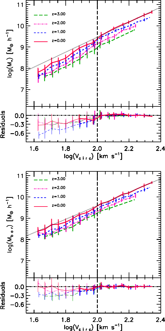
Figure 2:
The sTFR ( upper panels) and bTFR
( lower panels) in the S230 ( left)
and S230NF ( right) runs, at z = 0.
Grey symbols depict low-mass systems (
|
| Open with DEXTER | |
3 Results
We calculated the sTFR for our simulated galaxies by fitting a relation of the form
![]() .
In the case of the local sTFR in S230, we found a slope of
.
In the case of the local sTFR in S230, we found a slope of
![]() and
and
![]() ,
in general agreement
with observations (McGaugh et al. 2000; Bell & de Jong 2001).
As can be seen from Fig. 2
(upper left panel), the residuals of the linear fit to the relation
(small box) depart systematically from zero at around 100 km s-1, so that systems with lower circular velocities tend to
have lower stellar
masses than the predictions obtained from the fitting. Interestingly, this trend is consistent
with the observations reported by McGaugh et al. (2000) and Amorín et al. (2009)
and from theoretical expectations (Dekel & Silk 1986; Larson 1974).
To analyse to what extent SN feedback might be responsible for this
behaviour, we compared these findings with the ones obtained for S230NF
as shown in the upper right panel of Fig. 2.
We can appreciate that SN feedback seems to be crucial for reproducing
the observed features in the sTFR, since when this mechanism is turned
off, the simulated sTFR exhibits a linear behaviour
with a slope of
,
in general agreement
with observations (McGaugh et al. 2000; Bell & de Jong 2001).
As can be seen from Fig. 2
(upper left panel), the residuals of the linear fit to the relation
(small box) depart systematically from zero at around 100 km s-1, so that systems with lower circular velocities tend to
have lower stellar
masses than the predictions obtained from the fitting. Interestingly, this trend is consistent
with the observations reported by McGaugh et al. (2000) and Amorín et al. (2009)
and from theoretical expectations (Dekel & Silk 1986; Larson 1974).
To analyse to what extent SN feedback might be responsible for this
behaviour, we compared these findings with the ones obtained for S230NF
as shown in the upper right panel of Fig. 2.
We can appreciate that SN feedback seems to be crucial for reproducing
the observed features in the sTFR, since when this mechanism is turned
off, the simulated sTFR exhibits a linear behaviour
with a slope of ![]() 3, in agreement with theoretical predictions.
We can also see that the wind-free run predicts higher stellar masses for systems at a given circular
velocity, since it cannot regulate the transformation of gas into stars, which is too efficient in hydrodynamical simulations.
3, in agreement with theoretical predictions.
We can also see that the wind-free run predicts higher stellar masses for systems at a given circular
velocity, since it cannot regulate the transformation of gas into stars, which is too efficient in hydrodynamical simulations.
We also studied the bTFR in S230 and S230NF (Fig. 2, lower panels). The bTFR is obtained by adding
all baryons within
![]() ,
regardless of its physical state.
We can see that both models (with and without SN feedback) predict a linear
trend for the bTFR, at least, for the range of velocities covered by these simulations.
At z=0, the simulated bTFR in S230 has a slope of
,
regardless of its physical state.
We can see that both models (with and without SN feedback) predict a linear
trend for the bTFR, at least, for the range of velocities covered by these simulations.
At z=0, the simulated bTFR in S230 has a slope of
![]() and
and
![]() .
These values are generally in good agreement with observational results reported for late and early type
galaxies (Gurovich et al. 2010; De Rijcke et al. 2007). However, we warn that the comparison with observations is tricky since
we sum up the total amount of gas, while observers are limited by the instrumental techniques
that only give access to gas mass with certain physical properties.
For S230NF, the bTFR has a higher value of Y100 because these galaxies have been able to
retain their baryons in the central regions since no SN-driven outflows could be triggered. Also, S230NF
yields similar fittings to the sTFR and bTFR, indicating that stars dominate
the baryonic phase at this redshift.
.
These values are generally in good agreement with observational results reported for late and early type
galaxies (Gurovich et al. 2010; De Rijcke et al. 2007). However, we warn that the comparison with observations is tricky since
we sum up the total amount of gas, while observers are limited by the instrumental techniques
that only give access to gas mass with certain physical properties.
For S230NF, the bTFR has a higher value of Y100 because these galaxies have been able to
retain their baryons in the central regions since no SN-driven outflows could be triggered. Also, S230NF
yields similar fittings to the sTFR and bTFR, indicating that stars dominate
the baryonic phase at this redshift.
As already mentioned, the previous analysis was done by
using the value of
![]() at
at
![]() as a kinematical indicator.
To analyse the dependance of our results on the particular choice of the radius
at which we measure
as a kinematical indicator.
To analyse the dependance of our results on the particular choice of the radius
at which we measure
![]() ,
we also compared the relations obtained by using
,
we also compared the relations obtained by using
![]() evaluated at
evaluated at
![]() and
and
![]() .
We also estimated the maximum value of the rotation curve
.
We also estimated the maximum value of the rotation curve
![]() as can be seen
from Fig. 3.
The simulated sTFR and bTFR are not
significantly affected by variations in the radius at which
as can be seen
from Fig. 3.
The simulated sTFR and bTFR are not
significantly affected by variations in the radius at which
![]() is estimated. The largest changes with respect to our previous results (Fig. 2)
are obtained when using
is estimated. The largest changes with respect to our previous results (Fig. 2)
are obtained when using
![]() at
at
![]() as the velocity estimator.
Nevertheless, all changes remain within
a
as the velocity estimator.
Nevertheless, all changes remain within
a ![]() .
It is also worth noting that, in these simulations,
.
It is also worth noting that, in these simulations,
![]() at
at
![]() constitutes
a good proxy for the velocity
constitutes
a good proxy for the velocity
![]() ,
which is commonly employed in many
observational works.
Tables 2 and 3 summarize the
parameters corresponding to the linear
fits to the high-mass end (
,
which is commonly employed in many
observational works.
Tables 2 and 3 summarize the
parameters corresponding to the linear
fits to the high-mass end (
![]() )
of the TFRs shown in Fig. 3.
We can appreciate that, in all cases, the values of
)
of the TFRs shown in Fig. 3.
We can appreciate that, in all cases, the values of ![]() and Y100 agree within
a
and Y100 agree within
a ![]() .
Regarding the characteristic velocity where the sTFR bends, our findings suggest that
it does not depend on the particular kinematical estimators tested in this paper (Fig. 3, small boxes).
In light of these results, we hereafter use
.
Regarding the characteristic velocity where the sTFR bends, our findings suggest that
it does not depend on the particular kinematical estimators tested in this paper (Fig. 3, small boxes).
In light of these results, we hereafter use
![]() at
at
![]() as the kinematical indicator for our calculations.
as the kinematical indicator for our calculations.

|
Figure 3:
Mean sTFR ( left panel), bTFR ( right panel), and the corresponding standard
deviations for S230 at z=0. Results obtained by using
different kinematic indicators are compared:
|
| Open with DEXTER | |
Table 2:
Results of the linear fits
to the high-mass end (
![]() )
of the sTFR
for S230 at z=0.
)
of the sTFR
for S230 at z=0.
Table 3:
Results of the linear fits
to the high-mass end (
![]() )
of the bTFR
for S230 at z=0.
)
of the bTFR
for S230 at z=0.
By comparing the sTFR and bTFR in S230, it is clear that adding the gas
mass in the calculations contributes to restoring the linearity of the TFR over a wider velocity range.
These findings
suggest that, at ![]() ,
the bend of the local sTFR
might be partially caused by a decrease in the star formation
rate in smaller systems as a consequence of the gas heating by SNe.
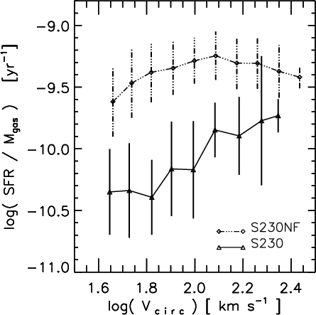
To quantify to what extent SN feedback can generate a decrease in the star formation
activity of simulated galaxies, we calculated the star formation efficiency (eSFR) defined as
the ratio of the star formation rate of a given galaxy to the total amount of gas contained within it.
In Fig. 4, we compare the mean eSFR as a function of
,
the bend of the local sTFR
might be partially caused by a decrease in the star formation
rate in smaller systems as a consequence of the gas heating by SNe.
To quantify to what extent SN feedback can generate a decrease in the star formation
activity of simulated galaxies, we calculated the star formation efficiency (eSFR) defined as
the ratio of the star formation rate of a given galaxy to the total amount of gas contained within it.
In Fig. 4, we compare the mean eSFR as a function of
![]() for galaxies in S230 and S230NF at z=0.
As expected, the model that includes SN feedback predicts smaller eSFRs at a
given
for galaxies in S230 and S230NF at z=0.
As expected, the model that includes SN feedback predicts smaller eSFRs at a
given
![]() ,
with slowly rotating systems exhibiting the most important variations,
on average. These systems still have an important percentage of gas but
it is in the form of a diffuse warm environment that does not fulfil
the conditions for forming stars.
,
with slowly rotating systems exhibiting the most important variations,
on average. These systems still have an important percentage of gas but
it is in the form of a diffuse warm environment that does not fulfil
the conditions for forming stars.
To analyse the evolution of both the sTFR and bTFR as a function of redshift,
we performed linear fits to the fast rotators using the characteristic velocity
![]() as a reference value at each analysed redshift.
As can be seen in Fig. 5, the residuals of the sTFR show a systematic departure from zero already from
as a reference value at each analysed redshift.
As can be seen in Fig. 5, the residuals of the sTFR show a systematic departure from zero already from
![]() ,
which occurs at approximately a similar characteristic velocity of
,
which occurs at approximately a similar characteristic velocity of ![]()
![]() .
For this SN model, we detect an evolution in the Y100 of the sTFR of
.
For this SN model, we detect an evolution in the Y100 of the sTFR of
![]() 0.44 dex since
0.44 dex since
![]() ,
while the
slope of the fast-rotating systems
remains almost constant.
In the case of the bTFR, Y100 evolves by around
,
while the
slope of the fast-rotating systems
remains almost constant.
In the case of the bTFR, Y100 evolves by around ![]() 0.30 dex between z=3 and z=0.
In particular, as can be appreciated from Fig. 5, the simulated bTFR retains the linear
relation over a wider velocity range. At z =0, there is no clear signal for a change in the slope within the numerical dispersion.
This finding is not in conflict with the recent observational results of McGaugh et al. (2010),
who report a break in the bTFR at
0.30 dex between z=3 and z=0.
In particular, as can be appreciated from Fig. 5, the simulated bTFR retains the linear
relation over a wider velocity range. At z =0, there is no clear signal for a change in the slope within the numerical dispersion.
This finding is not in conflict with the recent observational results of McGaugh et al. (2010),
who report a break in the bTFR at ![]() 20 km s-1,
because our simulations do not numerically resolve such low velocity systems.
While better statistics and higher
numerical resolution are needed to test the behaviour of the bTFR for low-velocity
systems, more detailed observations are also required to robustly probe the existence of the bend in the bTFR.
With regard to the S230NF, both the sTFR and the bTFR exhibit a linear trend from z=3 with no significant changes
in the slope but with an evolution of
20 km s-1,
because our simulations do not numerically resolve such low velocity systems.
While better statistics and higher
numerical resolution are needed to test the behaviour of the bTFR for low-velocity
systems, more detailed observations are also required to robustly probe the existence of the bend in the bTFR.
With regard to the S230NF, both the sTFR and the bTFR exhibit a linear trend from z=3 with no significant changes
in the slope but with an evolution of ![]() 0.55
in Y100, which is consistent with the higher eSFR measured in the galaxies in this run.
Both TFRs show larger dispersion for low-velocity rotators, which are also more
gas rich than systems at the high-velocity end.
At a given velocity,
slow rotators can have different baryonic and stellar masses, indicating their
different evolutionary paths. This behaviour can be also seen in S230NF albeit weaker, so
the dispersion has at least two causes: the different evolutionary paths
at a given circular velocity that regulate the transformation of gas into stars and
the action of SN feedback.
0.55
in Y100, which is consistent with the higher eSFR measured in the galaxies in this run.
Both TFRs show larger dispersion for low-velocity rotators, which are also more
gas rich than systems at the high-velocity end.
At a given velocity,
slow rotators can have different baryonic and stellar masses, indicating their
different evolutionary paths. This behaviour can be also seen in S230NF albeit weaker, so
the dispersion has at least two causes: the different evolutionary paths
at a given circular velocity that regulate the transformation of gas into stars and
the action of SN feedback.
|
Figure 4:
Mean star formation efficiency (eSFR) as a function of
|
| Open with DEXTER | |
|
Figure 5:
The evolution of the mean sTFR (upper panel) and bTFR
( lower panel) as a function of redshift
for S230 for z=3,2,1, and 0. The dotted black lines correspond to the fittings to the simulated TFRs for systems with
|
| Open with DEXTER | |
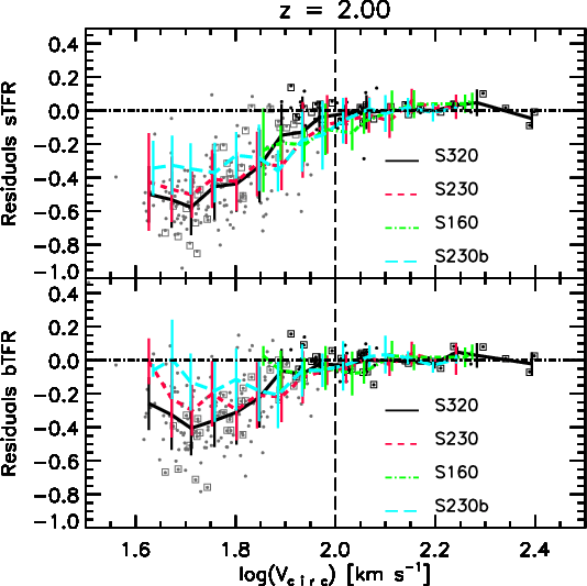
To assess the effects of numerical resolution on the determination of
characteristic velocity
![]() ,
we performed linear fits to the massive end (
,
we performed linear fits to the massive end (
![]() )
of the
sTFR and bTFR in S320, S230, and S160 at z = 2.0.
In Fig. 6,
we compare the mean values and standard deviations of the residuals
associated to
each simulation. We also show the results for S320. As can be
seen, the trend for the sTFR is clearly present in all simulations,
showing a change in the slope at a similar velocity.
With respect to the bTFR, it also exhibits a bend in the residuals at
around
)
of the
sTFR and bTFR in S320, S230, and S160 at z = 2.0.
In Fig. 6,
we compare the mean values and standard deviations of the residuals
associated to
each simulation. We also show the results for S320. As can be
seen, the trend for the sTFR is clearly present in all simulations,
showing a change in the slope at a similar velocity.
With respect to the bTFR, it also exhibits a bend in the residuals at
around ![]()
![]() at
at ![]() ,
but the
trend is weaker than for the sTFR.
The three simulations agree on the existence of the departure from linearity at
approximately the same velocity.
In the three runs, we also find larger dispersions for low-velocity rotators.
The agreement between the three different resolution-level simulations
suggests that these results are robust against numerical artefacts.
,
but the
trend is weaker than for the sTFR.
The three simulations agree on the existence of the departure from linearity at
approximately the same velocity.
In the three runs, we also find larger dispersions for low-velocity rotators.
The agreement between the three different resolution-level simulations
suggests that these results are robust against numerical artefacts.
Finally, since the SN feedback model uses
![]() K (equivalent to
K (equivalent to
![]() ,
where
,
where
![]() is the virial velocity of the halo)
as a parameter to separate cold and hot gas-phases surrounding
stellar populations, we evaluated how far this selection can influence the
determination of the characteristic velocity where the sTFR bends.
To assess this issue, we performed an extra simulation (S230b) with the same
initial conditions and SN and star formation parameters of S230, except for
is the virial velocity of the halo)
as a parameter to separate cold and hot gas-phases surrounding
stellar populations, we evaluated how far this selection can influence the
determination of the characteristic velocity where the sTFR bends.
To assess this issue, we performed an extra simulation (S230b) with the same
initial conditions and SN and star formation parameters of S230, except for ![]() ,
which
was lowered to
,
which
was lowered to
![]() K (equivalent to
K (equivalent to
![]() ).
Figure 6 shows that for both TFRs the residuals of these simulations are very similar. Particularly, both simulations predict
a bend at
).
Figure 6 shows that for both TFRs the residuals of these simulations are very similar. Particularly, both simulations predict
a bend at ![]()
![]() independently of the adopted value of
independently of the adopted value of
![]() ,
indicating that this parameter has no significant effect
of the determination of the bend.
,
indicating that this parameter has no significant effect
of the determination of the bend.
|
Figure 6:
Residuals corresponding to the
linear fits to the massive end (
|
| Open with DEXTER | |
4 Discussion
To further investigate our findings regarding the origin of the bend in the TFR and the role
played by SN feedback, we studied
the fraction
![]() for each simulated galaxy at z=0, where
for each simulated galaxy at z=0, where
![]() is the total mass within the virial radius
and i denotes the stellar or the baryonic component within
is the total mass within the virial radius
and i denotes the stellar or the baryonic component within
![]() .
The quantity f* (
.
The quantity f* (![]() )
therefore
represents the ratio between the stellar (baryonic) mass in a given galaxy and the expected
baryonic mass within the virial radius inferred from the universal baryonic fraction (
)
therefore
represents the ratio between the stellar (baryonic) mass in a given galaxy and the expected
baryonic mass within the virial radius inferred from the universal baryonic fraction (
![]() )
corresponding to the adopted cosmological parameters.
As can be appreciated from Fig. 7, f* is an increasing function of the circular velocity that, in its turn, is a measure of the potential well of the systems.
The small systems tend to have
f* < 0.1 at z = 0, while f* reaches
)
corresponding to the adopted cosmological parameters.
As can be appreciated from Fig. 7, f* is an increasing function of the circular velocity that, in its turn, is a measure of the potential well of the systems.
The small systems tend to have
f* < 0.1 at z = 0, while f* reaches ![]() 0.3
for more massive galaxies.
These findings are consistent with the fact that SN outflows are more
efficient to heat up and/or expel
the gas content from star-forming regions in shallower potential wells,
leading to a decrease in their stellar mass content and making them lie
below the sTFR determined by massive galaxies.
At z =2, the trends are similar to the local ones with faster rotators systems exhibiting stellar fractions of around 0.4 and
most of the slow rotators not exceeding 0.2.
Nonetheless, at a given circular velocity, the discrepancies between the simulated stellar components and the
theoretical baryonic masses
are more significant in the local Universe, showing the accumulated effects of SN feedback.
We also note that high redshift galaxies show a higher slope for the relation between
f* and
0.3
for more massive galaxies.
These findings are consistent with the fact that SN outflows are more
efficient to heat up and/or expel
the gas content from star-forming regions in shallower potential wells,
leading to a decrease in their stellar mass content and making them lie
below the sTFR determined by massive galaxies.
At z =2, the trends are similar to the local ones with faster rotators systems exhibiting stellar fractions of around 0.4 and
most of the slow rotators not exceeding 0.2.
Nonetheless, at a given circular velocity, the discrepancies between the simulated stellar components and the
theoretical baryonic masses
are more significant in the local Universe, showing the accumulated effects of SN feedback.
We also note that high redshift galaxies show a higher slope for the relation between
f* and ![]() indicating the more important action of SN winds on smaller systems at this epoch.
indicating the more important action of SN winds on smaller systems at this epoch.
When the gas mass within
![]() is incorporated into the calculations, we obtained the total baryonic fraction
is incorporated into the calculations, we obtained the total baryonic fraction ![]() .
At z=0,
.
At z=0, ![]() shows a weaker dependence on circular velocities than f*.
More massive galaxies exhibit
shows a weaker dependence on circular velocities than f*.
More massive galaxies exhibit
![]() ,
indicating that these systems are gas poor.
On the other hand, small galaxies exhibit baryonic fractions
,
indicating that these systems are gas poor.
On the other hand, small galaxies exhibit baryonic fractions ![]() that are more than half the value of f*.
These correlations explain the trend to recovering a single-slope
relation for the local TFR over a broader velocity range when
considering the baryonic content of galaxies instead of their stellar
mass. However, that
that are more than half the value of f*.
These correlations explain the trend to recovering a single-slope
relation for the local TFR over a broader velocity range when
considering the baryonic content of galaxies instead of their stellar
mass. However, that
![]() within
within
![]() for our whole sample indicates that galactic outflows are important over the whole simulated sample.
The effects on the faster rotators are also indirect since they grow by the accretion
of smaller substructures, which are strongly affected by SN feedback, as shown before.
The f* and
for our whole sample indicates that galactic outflows are important over the whole simulated sample.
The effects on the faster rotators are also indirect since they grow by the accretion
of smaller substructures, which are strongly affected by SN feedback, as shown before.
The f* and ![]() predicted by simulations qualitatively agree with observations (e.g. McGaugh et al. 2010), albeit with a weaker dependence on M*.
At z = 2, on the other hand, we obtained a stronger correlation between
predicted by simulations qualitatively agree with observations (e.g. McGaugh et al. 2010), albeit with a weaker dependence on M*.
At z = 2, on the other hand, we obtained a stronger correlation between ![]() and
and
![]() .
Slow-rotating systems at this redshift
show, on average, similar values of
.
Slow-rotating systems at this redshift
show, on average, similar values of ![]() to local ones. Conversely,
fast rotators in the local Universe
exhibit half of the baryonic fractions derived for systems of similar circular velocities at z
= 2. This behaviour is consistent with the stronger signal for a bend
in the bTFR that we found at high redshifts and shows that SN feedback
has acted on these systems
by expelling part of the baryonic mass outside the very central regions
from
to local ones. Conversely,
fast rotators in the local Universe
exhibit half of the baryonic fractions derived for systems of similar circular velocities at z
= 2. This behaviour is consistent with the stronger signal for a bend
in the bTFR that we found at high redshifts and shows that SN feedback
has acted on these systems
by expelling part of the baryonic mass outside the very central regions
from ![]() .
.
To estimate whether the expelled baryonic mass is within the virial radius
or if SN outflows have been powerful enough to transport it into the intergalactic medium (IGM),
we calculated the
fraction
![]() of the total baryonic mass within the virial radius of simulated galaxies
relative to the one derived from the universal baryonic fraction (
of the total baryonic mass within the virial radius of simulated galaxies
relative to the one derived from the universal baryonic fraction (
![]() )
in the
adopted cosmology. The results can
be appreciated in the right hand panels of Fig. 7.
By comparing these findings with the ones obtained for
)
in the
adopted cosmology. The results can
be appreciated in the right hand panels of Fig. 7.
By comparing these findings with the ones obtained for ![]() ,
it
is clear that a large amount of the missing baryons within
,
it
is clear that a large amount of the missing baryons within
![]() can be found in the surrounding halo. However, given that
can be found in the surrounding halo. However, given that
![]() ,
there is also a percentage of the gas blown away as a consequence
of very efficient galactic winds.
These effects are more evident at lower redshifts and for smaller systems.
,
there is also a percentage of the gas blown away as a consequence
of very efficient galactic winds.
These effects are more evident at lower redshifts and for smaller systems.
We can also see that the correlation with virial mass
is clearly defined at both redshifts though with high dispersion.
At z = 2, the percentage of absent baryons within
![]() ranges from 20% to 70%,
with slow rotators having experienced the most significant losses, as expected.
In the case of local galaxies, the percentage of lost baryons is within
the range 30% and 80%.
ranges from 20% to 70%,
with slow rotators having experienced the most significant losses, as expected.
In the case of local galaxies, the percentage of lost baryons is within
the range 30% and 80%.

|
Figure 7:
Left and middle panels:
Fraction of stellar (f*) and baryonic ( |
| Open with DEXTER | |
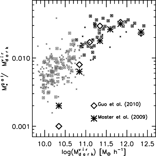
|
Figure 8: Fraction of stellar mass residing in simulated galaxies at z=0 relative to the dark component within the virial radius. For symbol codes see Fig. 2. We show for comparison results from the semi-analytical works by Guo et al. (2010) and Moster et al. (2009), as indicated in the figure. The vertical axis has been plotted using logarithmic scale. |
| Open with DEXTER | |
Finally, in Fig. 8, we contrast our findings to the trends obtained from the semi-empirical models of Guo et al. (2010) and Moster et al. (2009) which are derived from the observed luminosity function. This figure shows the fraction of stellar mass (F*) contained within each simulated galaxy at z=0 relative to the dark component within the virial radius. We see that there is very good agreement between our results and previous works. However, our model still tends to overpredict the stellar mass fractions at the low-mass end of the relation.
The dynamical evolution of galaxies in our simulations is driven by the
joint action of several physical processes, such as the star formation
mechanism, gas infall, and galactic outflows. The star formation
process is triggered mainly when the gas gets cold and dense![]() .
As a consequence of star formation, SN energy is released, thereby
heating up the surrounding cold and dense ISM, which when appropriated
(see Sect. 2), is promoted
to the hot phase.
This generates a stronger decrease in the star formation activity in
systems with shallower potential wells, because it is easier for the
cold and dense gas in small systems
to match the entropy of the hot and/or diffuse phase residing within their
small dark matter haloes.
But the cooling times (
.
As a consequence of star formation, SN energy is released, thereby
heating up the surrounding cold and dense ISM, which when appropriated
(see Sect. 2), is promoted
to the hot phase.
This generates a stronger decrease in the star formation activity in
systems with shallower potential wells, because it is easier for the
cold and dense gas in small systems
to match the entropy of the hot and/or diffuse phase residing within their
small dark matter haloes.
But the cooling times (
![]() )
of the promoted particles are
too short compared to their dynamical times (
)
of the promoted particles are
too short compared to their dynamical times (
![]() )
to allow this hot phase to be stable for a long time
)
to allow this hot phase to be stable for a long time![]() .
As a result, the gas that has just reached the hot phase due to SN
heating might cool down again on short timescales, returning to the
cold phase. Therefore, SN feedback leads to a self-regulated cycle of
heating and cooling, exerting a strong influence on the regulation of
the star formation process in low-mass galaxies. As the systems get
larger, the hot phase is established at a higher temperature owing to
the joint effect of the continuous pumping of SN energy into the hot
environment
and the increase in the virial temperature of the dark haloes hosting
them.
As the cooling times get longer than the dynamical time scales, the hot
gas is able to remain in this phase.
While the hot environment is able to build up as galaxies get more
massive, galactic winds are more difficult to be triggered in these
galaxies, since more SN energy would be required by the
cold phase to match the entropy of its nearby hot environment and,
therefore, to be promoted generating outflows. Meanwhile, the cold gas
remains available for star formation. It is also true that, as the
systems grow, their gas reservoir decreases, also decreasing their
star formation activity and, consequently, the source of
SN energy.
Therefore, the action of SN feedback is much less important for
regulating the transformation of the remaining gas into stars in these
large systems.
.
As a result, the gas that has just reached the hot phase due to SN
heating might cool down again on short timescales, returning to the
cold phase. Therefore, SN feedback leads to a self-regulated cycle of
heating and cooling, exerting a strong influence on the regulation of
the star formation process in low-mass galaxies. As the systems get
larger, the hot phase is established at a higher temperature owing to
the joint effect of the continuous pumping of SN energy into the hot
environment
and the increase in the virial temperature of the dark haloes hosting
them.
As the cooling times get longer than the dynamical time scales, the hot
gas is able to remain in this phase.
While the hot environment is able to build up as galaxies get more
massive, galactic winds are more difficult to be triggered in these
galaxies, since more SN energy would be required by the
cold phase to match the entropy of its nearby hot environment and,
therefore, to be promoted generating outflows. Meanwhile, the cold gas
remains available for star formation. It is also true that, as the
systems grow, their gas reservoir decreases, also decreasing their
star formation activity and, consequently, the source of
SN energy.
Therefore, the action of SN feedback is much less important for
regulating the transformation of the remaining gas into stars in these
large systems.
|
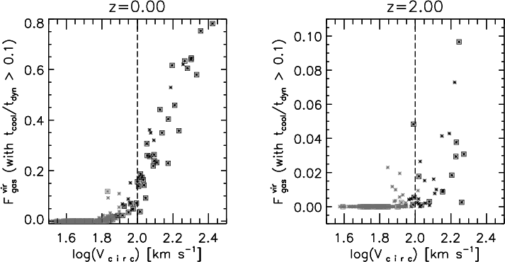
Figure 9:
Fraction of the gas component within
|
| Open with DEXTER | |
To quantitatively check that these behaviours are taking place in
our systems, we estimated the relations between the dynamical and the
cooling times of the cold gas that has joined the hot phase
by the action of SN feedback (i.e. promoted particles), during the
evolution of our simulated volumes.
The fraction of gas phase that is unavailable for efficient cooling
within simulated galaxies (
![]() )
is defined as the gas mass within
)
is defined as the gas mass within
![]() that satisfies the condition
that satisfies the condition
![]() (Navarro & White 1993).
In Fig. 9, we plot
(Navarro & White 1993).
In Fig. 9, we plot
![]() as a function of
as a function of
![]() in S230 at z=0 (left panel) and
z=2 (right panel).
As expected,
in S230 at z=0 (left panel) and
z=2 (right panel).
As expected,
![]() is an increasing function of
is an increasing function of
![]() .
At z=0, systems with
.
At z=0, systems with
![]() have a significant
percentage of their gas phase (>90%) subject to efficient cooling.
Only at
have a significant
percentage of their gas phase (>90%) subject to efficient cooling.
Only at
![]() does
does
![]() start to increase, reaching 0.8 at
start to increase, reaching 0.8 at
![]() .
The same trends are present at z =2, albeit with a larger dispersion at the
high-velocity end.
Interestingly, our model predicts that the transition from efficient to inefficient gas cooling occurs
at around the characteristic velocity
.
The same trends are present at z =2, albeit with a larger dispersion at the
high-velocity end.
Interestingly, our model predicts that the transition from efficient to inefficient gas cooling occurs
at around the characteristic velocity
![]() where
the TFR bends. This velocity also agrees with
the theoretical expectations from Dekel & Silk (1986), who concluded that,
only for systems with
where
the TFR bends. This velocity also agrees with
the theoretical expectations from Dekel & Silk (1986), who concluded that,
only for systems with
![]() larger than
larger than ![]()
![]() are
the cooling times of the diffuse and hot gas at least one order of magnitude longer than the
dynamical times and, therefore, the gas could remain hot.
are
the cooling times of the diffuse and hot gas at least one order of magnitude longer than the
dynamical times and, therefore, the gas could remain hot.
5 Conclusions
We have studied the sTFR and bTFR by performing hydrodynamical simulations in a cosmological scenario
including the action of the combined multiphase and SN feedback model of Scannapieco et al. (2006,2005).
Our results suggest there is a change in the slope of the sTFR and bTFR produced by the
action of SN feedback.
At z=0, the simulated sTFR is very tightly defined and in general
agreement with observations (e.g. McGaugh et al. 2000).
We detect a systematical change in the slope of the sTFR from approximately
![]()
![]() ,
at least since z=3,
so that
lower velocity systems tend to have lower stellar masses than those
predicted by the linear regression of the fast rotators.
The comparison with higher and lower resolution runs shows that this
feature is not just a numerical artefact. Regarding the local bTFR,
over the velocity range resolved by our simulations, it can be fitted
by a single linear model. At higher redshifts, we detect a weak trend
toward a change in the slope.
Similar trends are found by using
,
at least since z=3,
so that
lower velocity systems tend to have lower stellar masses than those
predicted by the linear regression of the fast rotators.
The comparison with higher and lower resolution runs shows that this
feature is not just a numerical artefact. Regarding the local bTFR,
over the velocity range resolved by our simulations, it can be fitted
by a single linear model. At higher redshifts, we detect a weak trend
toward a change in the slope.
Similar trends are found by using
![]() as the kinematical estimator.
as the kinematical estimator.
Our results suggest an evolution of ![]() 0.44 dex from z=3 to z=0 for the sTFR, which is consistent with what is reported by Cresci et al. (2009) of
0.44 dex from z=3 to z=0 for the sTFR, which is consistent with what is reported by Cresci et al. (2009) of
![]() dex from
dex from
![]() to z=0. For the baryonic relation, our model predicts a slightly weaker evolution of
to z=0. For the baryonic relation, our model predicts a slightly weaker evolution of ![]() 0.30 dex from z=3 to z=0.
In the wind-free run, both the sTFR and the bTFR show the same level of evolution
(
0.30 dex from z=3 to z=0.
In the wind-free run, both the sTFR and the bTFR show the same level of evolution
(![]() 0.55 dex), as expected since
baryons are efficiently transformed into stars as soon as they collapse within the potential well of a galaxy.
0.55 dex), as expected since
baryons are efficiently transformed into stars as soon as they collapse within the potential well of a galaxy.
The characteristic velocity of ![]()
![]() appears naturally
as a consequence of
the physically motivated multiphase and SN feedback treatment adopted
in these simulations. This model is successful at establishing a
self-regulated
star formation process without using any global properties of the
systems but resorting to the local
estimations of the thermodynamical properties of the gas in the
distinct components of the ISM.
We checked that this result is robust against variations in the SN
input parameters. Nevertheless, we acknowledge that there are several
open questions that need to be solved in the future such as the level
of change in the slope, which seems to be weaker in our simulations
than in observations. In this regard, our findings suggest that the
study of the sTFR and bTFR at different cosmic times could help
constrain SN feedback models.
appears naturally
as a consequence of
the physically motivated multiphase and SN feedback treatment adopted
in these simulations. This model is successful at establishing a
self-regulated
star formation process without using any global properties of the
systems but resorting to the local
estimations of the thermodynamical properties of the gas in the
distinct components of the ISM.
We checked that this result is robust against variations in the SN
input parameters. Nevertheless, we acknowledge that there are several
open questions that need to be solved in the future such as the level
of change in the slope, which seems to be weaker in our simulations
than in observations. In this regard, our findings suggest that the
study of the sTFR and bTFR at different cosmic times could help
constrain SN feedback models.
We thank the anonymous referee for his/her useful comments that largely helped to improve this paper. The authors are grateful to Cecilia Scannapieco for making the S320 simulation available and to Tomás Tecce for useful discussions. We acknowledge support from the PICT 32342 (2005) and PICT 245-Max Planck (2006) of ANCyT (Argentina). Simulations were run in Fenix and HOPE clusters at IAFE and Cecar cluster at University of Buenos Aires.
References
- Amorín, R., Aguerri, J. A. L., Muñoz-Tuñón, C., & Cairós, L. M. 2009, A&A, 501, 75 [NASA ADS] [CrossRef] [EDP Sciences] [Google Scholar]
- Avila-Reese, V., Firmani, C., & Hernández, X. 1998, ApJ, 505, 37 [NASA ADS] [CrossRef] [Google Scholar]
- Avila-Reese, V., Zavala, J., Firmani, C., & Hernández-Toledo, H. M. 2008, AJ, 136, 1340 [NASA ADS] [CrossRef] [Google Scholar]
- Bell, E. F., & de Jong, R. S. 2001, ApJ, 550, 212 [NASA ADS] [CrossRef] [Google Scholar]
- Conselice, C. J., Bundy, K., Ellis, R. S., et al. 2005, ApJ, 628, 160 [NASA ADS] [CrossRef] [Google Scholar]
- Cresci, G., Hicks, E. K. S., Genzel, R., et al. 2009, ApJ, 697, 115 [NASA ADS] [CrossRef] [Google Scholar]
- Croft, R. A. C., Di Matteo, T., Springel, V., & Hernquist, L. 2009, MNRAS, 400, 43 [NASA ADS] [CrossRef] [Google Scholar]
- De Rijcke, S., Zeilinger, W. W., Hau, G. K. T., Prugniel, P., & Dejonghe, H. 2007, ApJ, 659, 1172 [NASA ADS] [CrossRef] [Google Scholar]
- Dekel, A., & Silk, J. 1986, ApJ, 303, 39 [NASA ADS] [CrossRef] [Google Scholar]
- Dutton, A. A., & van den Bosch, F. C. 2009, MNRAS, 396, 141 [NASA ADS] [CrossRef] [Google Scholar]
- Flores, H., Hammer, F., Puech, M., Amram, P., & Balkowski, C. 2006, A&A, 455, 107 [NASA ADS] [CrossRef] [EDP Sciences] [Google Scholar]
- Governato, F., Willman, B., Mayer, L., et al. 2007, MNRAS, 374, 1479 [NASA ADS] [CrossRef] [Google Scholar]
- Governato, F., Brook, C., Mayer, L., et al. 2010, Nature, 463, 203 [NASA ADS] [CrossRef] [PubMed] [Google Scholar]
- Guo, Q., White, S., Li, C., & Boylan-Kolchin, M. 2010, MNRAS, 404, 1111 [NASA ADS] [Google Scholar]
- Gurovich, S., McGaugh, S. S., Freeman, K. C., et al. 2004, PASA, 21, 412 [Google Scholar]
- Gurovich, S., Freeman, K. C., Jerjen, H., Staveley-Smith, L., & Puerani, I. 2010, AJ, 140, 663 [NASA ADS] [CrossRef] [Google Scholar]
- Kang, X., Jing, Y. P., Mo, H. J., & Borner, G. 2005, ApJ, 631, 21 [NASA ADS] [CrossRef] [Google Scholar]
- Larson, R. B. 1974, MNRAS, 169, 229 [NASA ADS] [CrossRef] [Google Scholar]
- Mac Low, M. M., & Ferrara, A. 1999, ApJ, 513, 142 [NASA ADS] [CrossRef] [Google Scholar]
- McGaugh, S. S. 2005, ApJ, 632, 859 [NASA ADS] [CrossRef] [Google Scholar]
- McGaugh, S. S., Schombert, J. M., Bothun, G. D., & de Blok, W. J. G. 2000, ApJ, 533, L99 [NASA ADS] [CrossRef] [PubMed] [Google Scholar]
- McGaugh, S. S., Schombert, J. M., de Blok, W. J. G., & Zagursky, M. J. 2010, ApJ, 708L, 14 [Google Scholar]
- Mo, H. J., Mao, S., & White, S. D. M. 1998, MNRAS, 295, 319 [Google Scholar]
- Mosconi, M. B., Tissera, P. B., Lambas, D. G., & Cora, S. A. 2001, MNRAS, 325, 34 [NASA ADS] [CrossRef] [Google Scholar]
- Moster, B. P., Somerville, R. S., Maulbetsch, C., et al. 2009, ApJ, 710, 903 [Google Scholar]
- Nagashima, M., Yahagi, H., Enoki, M., Yoshii, Y., & Gouda, N. 2005, ApJ, 634, 26 [NASA ADS] [CrossRef] [Google Scholar]
- Puech, M., Hammer, F., Flores, H., et al. 2010, A&A, 510, 68 [Google Scholar]
- Raiteri, C. M., Villata, M., & Navarro, J. F. 1996, A&A, 315, 105 [NASA ADS] [Google Scholar]
- Scannapieco, C., Tissera, P. B., White, S. D. M., & Springel, V. 2005, MNRAS, 364, 552 [NASA ADS] [CrossRef] [Google Scholar]
- Scannapieco, C., Tissera, P. B., White, S. D. M., & Springel, V. 2006, MNRAS, 371, 1125 [NASA ADS] [CrossRef] [Google Scholar]
- Scannapieco, C., Tissera, P. B., White, S. D. M., & Springel, V. 2008, MNRAS, 389, 1137 [NASA ADS] [CrossRef] [Google Scholar]
- Springel, V. 2005, MNRAS, 364, 1105 [NASA ADS] [CrossRef] [Google Scholar]
- Springel, V., & Hernquist, L. 2003, MNRAS, 339, 289 [Google Scholar]
- Springel, V., White, S. D. M., Tormen, G., & Kauffmann, G. 2001, MNRAS, 328, 726 [Google Scholar]
- Steinmetz, M., & Navarro, J. F. 1999, ApJ, 513, 555 [NASA ADS] [CrossRef] [Google Scholar]
- Stinson, G. S., Quinn, T., Dalcanton, J., Wadsley, J., & Gogarten, S. 2007, A&AS, 38, 766 [Google Scholar]
- Tassis, K., Kravtsov, A. V., & Gnedin, N. Y. 2008, ApJ, 672, 888 [NASA ADS] [CrossRef] [Google Scholar]
- Thielemann, F. K., Nomoto, K., & Hashimoto, M. 1993, in Origin and Evolution of the Elements, ed. N. Prantzoz, et al. (Cambridge University Press), 297 [Google Scholar]
- Tissera, P. B., Lambas, D. G., & Abadi, M. G. 1997, MNRAS, 286, 384 [NASA ADS] [Google Scholar]
- Tully, R. B., & Fisher, J. R. 1977, A&A, 54, 661 [NASA ADS] [Google Scholar]
- Verheijen, M. A. W. 2001, ApJ, 563, 694 [NASA ADS] [CrossRef] [Google Scholar]
- White, S. D. M., & Frenk, C. S. 1991, ApJ, 379, 52 [NASA ADS] [CrossRef] [Google Scholar]
- Woosley, S. E., & Weaver, T. A. 1995, ApJS, 101, 181 [NASA ADS] [CrossRef] [Google Scholar]
Footnotes
- ... SNII
![[*]](/icons/foot_motif.png)
- Scannapieco et al. (2005) also implemented a version that relax the IRA, assuming the age-mass-metallicity fitting polynomials estimated by Raiteri et al. (1996). However, no significant changes were found in the results compared to the IRA.
- ... dense
- Recall that in this model the cold phase is defined as the
gas component with temperature
 where
where  K
and density
K
and density  where
where  is
is  (Sect. 2).
Otherwise, the gas is classified as hot phase.
(Sect. 2).
Otherwise, the gas is classified as hot phase.
- ... time
- In our model, the cooling and dynamical times are
calculated following standard definitions as
 and
and
 ,
respectively.
,
respectively.
All Tables
Table 1: Cosmological hydrodynamical simulations studied in this paper.
Table 2:
Results of the linear fits
to the high-mass end (
![]() )
of the sTFR
for S230 at z=0.
)
of the sTFR
for S230 at z=0.
Table 3:
Results of the linear fits
to the high-mass end (
![]() )
of the bTFR
for S230 at z=0.
)
of the bTFR
for S230 at z=0.
All Figures
| |
Figure 1:
Projected gaseous mass distributions for a typical disc galaxy in a face-on view ( left panel) and an edge-on one ( middle panel) and the corresponding
|
| Open with DEXTER | |
| In the text | |
|
|
Figure 2:
The sTFR ( upper panels) and bTFR
( lower panels) in the S230 ( left)
and S230NF ( right) runs, at z = 0.
Grey symbols depict low-mass systems (
|
| Open with DEXTER | |
| In the text | |
|
|
Figure 3:
Mean sTFR ( left panel), bTFR ( right panel), and the corresponding standard
deviations for S230 at z=0. Results obtained by using
different kinematic indicators are compared:
|
| Open with DEXTER | |
| In the text | |
|
|
Figure 4:
Mean star formation efficiency (eSFR) as a function of
|
| Open with DEXTER | |
| In the text | |
|
|
Figure 5:
The evolution of the mean sTFR (upper panel) and bTFR
( lower panel) as a function of redshift
for S230 for z=3,2,1, and 0. The dotted black lines correspond to the fittings to the simulated TFRs for systems with
|
| Open with DEXTER | |
| In the text | |
|
|
Figure 6:
Residuals corresponding to the
linear fits to the massive end (
|
| Open with DEXTER | |
| In the text | |
|
|
Figure 7:
Left and middle panels:
Fraction of stellar (f*) and baryonic ( |
| Open with DEXTER | |
| In the text | |
|
|
Figure 8: Fraction of stellar mass residing in simulated galaxies at z=0 relative to the dark component within the virial radius. For symbol codes see Fig. 2. We show for comparison results from the semi-analytical works by Guo et al. (2010) and Moster et al. (2009), as indicated in the figure. The vertical axis has been plotted using logarithmic scale. |
| Open with DEXTER | |
| In the text | |
|
|
Figure 9:
Fraction of the gas component within
|
| Open with DEXTER | |
| In the text | |
Copyright ESO 2010
Current usage metrics show cumulative count of Article Views (full-text article views including HTML views, PDF and ePub downloads, according to the available data) and Abstracts Views on Vision4Press platform.
Data correspond to usage on the plateform after 2015. The current usage metrics is available 48-96 hours after online publication and is updated daily on week days.
Initial download of the metrics may take a while.