| Issue |
A&A
Volume 519, September 2010
|
|
|---|---|---|
| Article Number | A4 | |
| Number of page(s) | 14 | |
| Section | Astronomical instrumentation | |
| DOI | https://doi.org/10.1051/0004-6361/200912001 | |
| Published online | 06 September 2010 | |
Reconstruction of the cosmic microwave background lensing for Planck
L. Perotto1,2 - J. Bobin3,4 - S. Plaszczynski2 - J.-L. Starck3 - A. Lavabre2
1 - Laboratoire de Physique Subatomique et de Cosmologie (LPSC),
CNRS: UMR5821, IN2P3, Université Joseph Fourier -
Grenoble I, Institut Polytechnique de Grenoble, France
2 - Laboratoire de l'Accélérateur Linéaire (LAL), CNRS: UMR8607, IN2P3, Université Paris-Sud, Orsay, France
3 - Laboratoire AIM (UMR 7158), CEA/DSM-CNRS-Université Paris
Diderot, IRFU, SEDI-SAP, Service d'Astrophysique, Centre de Saclay,
91191 Gif-Sur-Yvette Cedex, France
4 - Applied and Computational Mathematics (ACM), California
Institute of Technology, 1200 E.California Bvd, M/C 217-50, PASADENA
CA-91125, USA
Received 6 March 2009 / Accepted 19 February 2010
Abstract
Aims. We prepare real-life cosmic microwave background (CMB) lensing extraction with the forthcoming Planck
satellite data by studying two systematic effects related to the
foreground contamination: the impact of foreground residuals after a
component separation on the lensed CMB map, and the impact of removing
a large contaminated region of the sky.
Methods. We first use the generalized morphological component
analysis (GMCA) method to perform a component separation within a
simplified framework, which allows a high statistics Monte-Carlo study.
For the second systematic, we apply a realistic mask on the temperature
maps and then restore them with a recently developed inpainting
technique on the sphere. We investigate the reconstruction of the CMB
lensing from the resultant maps using a quadratic estimator in the flat
sky limit and on the full sphere.
Results. We find that the foreground residuals from the GMCA
method does not significantly alter the lensed signal, which is also
true for the mask corrected with the inpainting method, even in the
presence of point source residuals.
Key words: cosmic microwave background - large-scale structure of Universe - gravitational lensing: weak - methods: statistical
1 Introduction
Cosmic microwave background (CMB) temperature anisotropies and polarization
measurements have been one of the key cosmological probes to establish the current cosmological constant
![]() and cold dark matter (
and cold dark matter (![]() CDM) paradigm. Reaching the most precise measurement
of these observables is
the main scientific goal of the forthcoming or ongoing CMB experiments - like the
European Spacial Agency satellite Planck
CDM) paradigm. Reaching the most precise measurement
of these observables is
the main scientific goal of the forthcoming or ongoing CMB experiments - like the
European Spacial Agency satellite Planck![]() ,
which was successfully launched on the 14th of May 2009 and has currently begun collecting data.
,
which was successfully launched on the 14th of May 2009 and has currently begun collecting data.
Planck is designed to deliver full-sky coverage, low-level noise, high resolution temperature and polarization maps (see Tauber 2006; The Planck Consortia 2005). With these high quality observations it will be possible to extract cosmological informations from the CMB maps beyond the angular power spectra (two-points correlations, hereafter APS), by exploiting the measurable non-Gaussianities (see e.g. The Planck Consortia 2005; Komatsu 2002).
The weak gravitational lensing is one of the sources of non-Gaussianity affecting the CMB after the recombination (see Lewis & Challinor 2006 for a review). The CMB photons are weakly deflected by the gravitational potential of the intervening large-scale structures (LSS), which perturb the Gaussian statistic of the CMB anisotropies (Zaldarriaga 2000; Bernardeau 1997). Conversely, it becomes possible to reconstruct the underlying gravitational potential by exploiting the higher-order correlations induced by the weak lensing in the CMB maps (Guzik et al. 2000; Hirata & Seljak 2003a; Hu 2001b; Takada & Futamase 2001; Bernardeau 1997).
The relevance of the CMB lensing reconstruction for the cosmology is twofold. First, for the sake of measuring the primordial B-mode of polarization predicted by the inflationary models (Seljak & Zaldarriaga 1997; Kamionkowski et al. 1997), the CMB lensing is a major contaminant. It induces a secondary B-mode polarization signal in perturbing the E-mode polarization pattern (Zaldarriaga & Seljak 1998). A lensing reconstruction allowing the delensing of the CMB maps is required to recover the primordial B-mode signal (Knox & Song 2002; Seljak & Hirata 2004). However, CMB lensing is also a powerful cosmological probe of the matter distribution integrated from the last scattering surface to us. This will soon be a unique opportunity to probe the full-sky LSS distribution, with a maximum efficiency at redshift around 3, where structures still experience a well described linear growth (Lewis & Challinor 2006). A lensing reconstruction would largely improve the sensitivity of the CMB experiments to the cosmological parameters that affect the growth of the LSS, like neutrino mass or dark energy (Lesgourgues et al. 2006; Kaplinghat et al. 2003; Perotto et al. 2006; Hu 2002).
Although well-known theoretically (Blanchard & Schneider 1987), the CMB lensing has never been directly
measured. Smith et al. (2007) and Hirata et al. (2008) have found evidence for a detection of the CMB
lensing in the WMAP data by correlating them with several other LSS probes (Luminous Red Galaxies,
Quasars and radio sources) at 3.4![]() and 2.5
and 2.5![]() level respectively. This situation is
expected to change with the forthcoming Planck data. Planck will be the first CMB
experiment allowing the measurement of the underlying gravitational potential without requiring
any external data. However, even with the never before met quality of the Planck data,
CMB lensing reconstruction will be challenging. The lensing of the CMB is a very subtle
secondary effect, affecting the smaller angular scale at the limit of the Planck
resolution in a correlated way over several degrees on the sky. As already quoted, its reconstruction is
based on the induced non-Gaussianities in the CMB maps in the form of mode
coupling. Consequently, any process resulting in coupling different Fourier moments is a challenging systematic to deal
with in order to retrieve the lensing signal (see Su & Yadav 2009 for a recent study of
the impact of instrumental systematics on the CMB lensing reconstruction bias).
Astrophysical components and other secondary effects could also be a source of non-Gaussianity. These components include
thermal and kinetic Sunyaev-Zel'dovich effects (thSZ and kSZ), due to the
scattering of CMB radiation by electrons within the galaxy clusters (Sunyaev & Zeldovich 1970); foreground emissions like synchrotron,
Bremsstrahlung and dust-diffuse galactic emission as well as extragalactic point
sources. All these components may give a sizable
contribution to the level of non-Gaussianities in the CMB maps (Babich & Pierpaoli 2008; Riquelme & Spergel 2007; Aghanim & Forni 1999; Argüeso et al. 2003; Amblard et al. 2004).
level respectively. This situation is
expected to change with the forthcoming Planck data. Planck will be the first CMB
experiment allowing the measurement of the underlying gravitational potential without requiring
any external data. However, even with the never before met quality of the Planck data,
CMB lensing reconstruction will be challenging. The lensing of the CMB is a very subtle
secondary effect, affecting the smaller angular scale at the limit of the Planck
resolution in a correlated way over several degrees on the sky. As already quoted, its reconstruction is
based on the induced non-Gaussianities in the CMB maps in the form of mode
coupling. Consequently, any process resulting in coupling different Fourier moments is a challenging systematic to deal
with in order to retrieve the lensing signal (see Su & Yadav 2009 for a recent study of
the impact of instrumental systematics on the CMB lensing reconstruction bias).
Astrophysical components and other secondary effects could also be a source of non-Gaussianity. These components include
thermal and kinetic Sunyaev-Zel'dovich effects (thSZ and kSZ), due to the
scattering of CMB radiation by electrons within the galaxy clusters (Sunyaev & Zeldovich 1970); foreground emissions like synchrotron,
Bremsstrahlung and dust-diffuse galactic emission as well as extragalactic point
sources. All these components may give a sizable
contribution to the level of non-Gaussianities in the CMB maps (Babich & Pierpaoli 2008; Riquelme & Spergel 2007; Aghanim & Forni 1999; Argüeso et al. 2003; Amblard et al. 2004).
The impact of most of the aforementioned effects on the CMB lensing analysis with WMAP data has been investigated by Hirata et al. (2008). They found a negligible contamination level, which is encouraging. However, such a result could change when one considers the higher resolution, better sensitivity maps provided by Planck. In Barreiro et al. (2006) the component separation impact on non-Gaussianity was studied in the framework of the Planck project, but no lensing reconstruction was performed. Hence the impact of these foreground residuals on the CMB lensing reconstruction is still to be studied.
The overall purpose of the present study is to give an insight to the issues we should deal with before undertaking any complete study of the CMB lensing retrieval with Planck: what is the impact of the foreground residuals on the CMB lensing reconstruction? Will it still be possible to reconstruct the CMB lensing after a component separation process, or will such a process alter the temperature map statistics? How should we deal with the masking issue? Beyond the detection of the CMB lensing signal, we tackled the reconstruction of the underlying projected potential APS. We investigated two issues, the impact of a component separation algorithm on the lensing reconstruction and the impact of a masked temperature map restoration before applying a deflection estimator.
Section 2 briefly reviews the CMB lensing effect and the reconstruction method. We present in Sect. 3 an analysis of the impact of one component separation technique, named generalized morphological component Analysis (GMCA) (Bobin et al. 2008), which is one of the different methods investigated by the Planck consortium (Leach et al. 2008). In Sect. 4, we show how a recently developed gap-filling method (i.e. inpainting process) (Abrial et al. 2008) may solve the masking problem, which may be one of the major issues for the CMB lensing retrieval because it introduces some misleading correlations between different angular scales in the maps.
2 CMB lensing
In this section, we briefly review the CMB lensing effect and the reconstruction method.
We introduce the notations used throughout this paper.
The geodesic of the CMB photons is weakly deflected by the gravitational potential from the last
scattering surface to us. Observationally this effect results in a remapping of the CMB
temperature anisotropies
![]() ,
according to Blanchard & Schneider (1987):
,
according to Blanchard & Schneider (1987):
In words, the lensed temperature
The CMB lensing probes the intervening mass in a broad range of redshifts,
from
z* = 1090 at the last scattering surface to z=0, with a maximum efficiency at ![]() .
At this high redshift, the LSS responsible for
the CMB lensing (with a typical scale of
.
At this high redshift, the LSS responsible for
the CMB lensing (with a typical scale of
![]() )
still
experience a linear regime of growth. As a result the projected potential
)
still
experience a linear regime of growth. As a result the projected potential ![]() can be assumed to be a
Gaussian random field. The consequences of the
nonlinear corrections to
can be assumed to be a
Gaussian random field. The consequences of the
nonlinear corrections to ![]() are shown to be weak on the CMB lensed
observables (Challinor & Lewis 2005). Thus, this hypothesis holds very well as long as the
CMB lensing study does not aim at measuring a correlation with other LSS probes at lower redshifts.
are shown to be weak on the CMB lensed
observables (Challinor & Lewis 2005). Thus, this hypothesis holds very well as long as the
CMB lensing study does not aim at measuring a correlation with other LSS probes at lower redshifts.
Besides, the deflection angles have a rms of ![]() 2.7 arcmin in the standard
2.7 arcmin in the standard ![]() CDM
model and can be correlated over several degrees on the sky. The
typical scales of the lensing effects are small enough for a convenient
analysis within the flat-sky approximation. The projected potential may
be decomposed on a Fourier basis
CDM
model and can be correlated over several degrees on the sky. The
typical scales of the lensing effects are small enough for a convenient
analysis within the flat-sky approximation. The projected potential may
be decomposed on a Fourier basis
![]() ,
and its statistics is completely defined by
,
and its statistics is completely defined by
|
(2) |
where

The lensed CMB temperature APS can be derived from the Fourier transform of Eq. (1) (e.g. as in Okamoto & Hu 2003). The lensing effect slightly modifies the APS of the CMB temperature, weakly smoothing the power at all angular scale to the benefit of the smaller angular scales. Deeply in the damping tail, at multipole
Consequently, the two-point correlation function of the lensed temperature modes, calculated at
the first order in ![]() ,
is written as (Okamoto & Hu 2003)
,
is written as (Okamoto & Hu 2003)
where
Similarly, one can calculate the four-point correlation function of the CMB temperature field - as in Kesden et al. (2003). One finds that the trispectrum of the lensed temperature field - or equivalently, the connected part of its four-point correlation function - is non-null even if the underlying (unlensed) temperature field is purely Gaussian.
Two possible ways were developed to deal with the reconstruction of the integrated gravitational potential field from a lensed CMB map. One was described by Hirata & Seljak (2003b,a), whose maximum-likelihood estimator method aims to increase the capabilities of the highest sensitivity highest resolution CMB projects in reconstructing the integrated potential. The other was developed by Okamoto & Hu (2003); Hu (2001b); Hu & Okamoto (2002), whose quadratic estimator approach is still close to optimal for currently built experiments like Planck. Accordingly we adopt this method throughout this work.
In the flat sky approximation, the estimated potential map takes the following form (Okamoto & Hu 2003):
where the Fourier modes
where
![\begin{displaymath}N_{k}^{{\rm TT}} ~ = ~ \theta_{{\rm fwhm}}^{~ 2} \sigma_{{\rm...
...exp \left[ k^2 \frac{\theta_{{\rm fwhm}}^{~2}}{8\ln 2}\right],
\end{displaymath}](/articles/aa/full_html/2010/11/aa12001-09/img42.png)
where
Besides, the normalization function is calculated so that
![]() is an
unbiased estimator of the integrated potential field
is an
unbiased estimator of the integrated potential field
![\begin{displaymath}A_{{\rm TT}}(L) ~=~ L^2 \left[ \int \frac{{\rm d}^2\vec k_1}{...
... k_1,\vec k_2)
F_{{\rm TT}}(\vec k_1,\vec k_2) \right]^{-1} ~.
\end{displaymath}](/articles/aa/full_html/2010/11/aa12001-09/img46.png)
Then the weighting function
where
Finally, the covariance of the integrated potential field estimator provides us with a four-point estimator
of the integrated potential APS. When expanding the lensed CMB temperature modes at second
order in ![]() ,
the
,
the
![]() estimator covariance reads
estimator covariance reads
where the estimated potential APS,
Here we have distinguished three different noise contributions to the integrated potential estimator variance. The dominant noise contribution,
These two non-Gaussian noise terms arise from the trispectrum part (or so-called connected part) of the four-point lensed temperature correlator hidden in the integrated potential field estimator covariance. It can be interpreted as the confusion noise coming from other integrated potential modes. Because it depends on the integrated potential APS, which has to be estimated, an iterative estimation scheme would be required for taking it into account. However, our study based on simulated data allows us to calculate these terms from the fiducial potential APS and then subtract it from the estimator variance.
3 Effect of foreground removal: a Monte-Carlo analysis
Up to now, no analysis has been performed to assess the effect of a component separation process on the CMB lensing extraction. The question we propose to address here is whether the lensing signal is preserved in the CMB map output by the component separation process. In order to get a first insight, we use a Monte-Carlo approach within the flat sky approximation.
3.1 Idealized Planck sky model
We created a simulation pipeline to generate some idealized synthetic patches of the sky for the Planck experiment. Our sky model is a linear uncorrelated mixture of the lensed CMB temperature and astrophysical components, which includes the Sunyaev-Zel'dovich effect, the thermal emission of the interstellar dust and the unresolved infrared point sources emission. In modeling these three components, we made sure to catch the dominant foreground emission features at the Planck-HFI frequencies. Then we added the nominal effects of the Planck-HFI instrument, modeled as a purely Gaussian-shaped beam and a spatially uniform white Gaussian noise. Each hypothesis we adopted is a crude model of the astrophysical contaminant and systematic effects that pollute the Planck data, and is intended to be a demonstration model for a study devoted to the impact of the component separation algorithms on the CMB lensing retrieval.
We generated four sets of 300 Planck-HFI synthetic patches of the sky, with instrumental noise and, when needed, with foreground emissions.
- Set I contains lensed CMB temperature maps generated from an unique fixed projected potential realization and with the instrumental effects (beam and white noise);
- Set I-fg is built from Set I. In addition, a fixed realization of dust and SZ was added to each Set I map;
- Set II is a set of lensed CMB temperature maps generated from 300 random realizations of the lenses distribution plus the instrumental effects;
- Set II-fg is built from Set II. Each map of Set II is
superimposed with one of each foreground maps out of the
available 30 dust maps, located at high galactic latitude
(
 ), and 1500 SZ maps.
3.1.1 Lensed CMB temperature map
Once we assumed the Gaussianity of the integrated potential field, the lensed CMB temperature
simulation principle is straightforward as a direct application of the remapping
Eq. (1). We started from the APS of both the temperature and the
projected potential field as well as the cross-APS reflecting the correlation between the
CMB temperature and the gravitational potential fields due to the Integrated Sachs-Wolfe (ISW)
effect.
Then we generated two Gaussian fields directly in the Fourier space, so that
where
From CMB temperature and projected potential in the Fourier space, we calculated both the temperature
and the deflection angles in the real space. The last step consisted in performing the remapping of
the primordial temperature map according to the deflection angles. Here is the technical point.
Starting from a regular sample of a field (the underlying unlensed map), we have to extract an
irregular sample of the same field (the lensed map) - the new directions where to sample from are
given by the previous one shifted by the deflection angles. Thus, this is a well-documented
interpolation issue, the difficulty lying in the fact that the scale of the interpolation scheme
is the same as the typical scale of the physical process of interest. We took particular care in
the interpolation algorithm to avoid creating some spurious lensing signal or
introducing additional non-Gaussianities. We found that a parametric cubic interpolation
scheme (Park & Schowengerdt 1983) fitted reasonably well. In addition, to avoid any loss of power due to the
interpolation, we overpixellized twice the underlying unlensed temperature and deflection field.
The first test we performed to control the quality of the simulation was to compare the Monte-Carlo
estimate of the APS over 500 simulations of the lensed maps to the analytical
calculation of the lensed APS provided by the
CAMB![]() Boltzmann code (Challinor & Lewis 2005; Lewis et al. 2000).
As shown in Fig. 1, the APS of our simulated lensed maps is
consistent with the theoretical one up to multipole 4000 - which is large enough to study the CMB lensing with Planck.
Boltzmann code (Challinor & Lewis 2005; Lewis et al. 2000).
As shown in Fig. 1, the APS of our simulated lensed maps is
consistent with the theoretical one up to multipole 4000 - which is large enough to study the CMB lensing with Planck.
![\begin{figure}
\par\resizebox{9cm}{!}{\includegraphics[viewport= 0 0 566 407,clip]{12001fig/12001fig1}} \end{figure}](/articles/aa/full_html/2010/11/aa12001-09/img69.png)
|
Figure 1: CMB temperature APS. The red/black (respectively green/grey) line is the lensed (respectively unlensed) temperature APS calculated with the public Boltzmann code CAMB (Challinor & Lewis 2005; Lewis et al. 2000). The blue/black data-points are the mean of the binned power spectrum reconstructed on 500 simulated lensed temperature maps. The error-bars are given by the variance of the 500 APS estimates. |
| Open with DEXTER | |
3.1.2 Astrophysical components
In any CMB experiment the temperature signal is mixed with foreground contributions of astrophysical origin - among them we can separate the diffuse galactic emission (thermal and rotational dust, synchrotron, Bremsstrahlung (free-free) radiation) from the extragalactic components (point sources, thermal and kinetic Sunyaev-Zel'dovich effects). As discussed in the introduction, each of these components could potentially, if inefficiently removed, degrade our capability to reconstruct the CMB lensing. Here, to complete our demonstration sky model, we choose to simulate the dominant astrophysical foregrounds at the Planck-HFI frequencies, namely the thermal emission of the galactic dust, the thermal SZ effect and the unresolved infra-red point sources. Thermal dust templates are obtained from the 100Table 1:
Instrumental characteristics of Planck-HFI
![]() .
.
3.1.3 Planck-like noise
Finally, we simulated the effects of the Planck High Frequency Instrument (HFI) according
to their nominal characteristics (The Planck Consortia 2005), which are summarized
in Table 1. At each frequency channel, the component mixture was convolved with a
Gaussian beam with the corresponding FWHM size.
Then a spatially uniform white noise following a Gaussian statistic was added. Finally, the
resulting maps were deconvolved from the beam transfer function, resulting in an exponential
increase of the noise at the scales corresponding to the beam size. Because smaller angular
scales carry the larger amount of lensing information, the higher the angular resolution is, the
better the lensing reconstruction can be. Our tests show that in the ideal case the lensing
reconstruction on Planck-HFI synthetic maps is insensitive to the addition or the removal of
the 100 GHz frequency channel information, whose beam function is roughly
twice as large as the beam in the higher frequency channels. It was even worse when we ran the
full Monte-Carlo chain, because after turning the foreground emission and component separation
process on, the addition of the lower frequency channel resulted in increasing the confusion noise
of the lensing reconstruction. That was the reason we excluded the 100 GHz
frequency channel from our analysis. To summarize, our Planck sky model reads
|
(14) |
where
3.2 Component separation using the generalized morphological component analysis
For most of the cosmological analysis of the CMB data - and for the CMB lensing extraction in particular - the cosmological signal has to be carefully disentangled from the other sources of emission that contribute to the observed temperature map. The component separation is a part of the signal processing dedicated to distinguish between the different contributions of the final maps. Briefly, the gist of any component separation technique consists in taking advantage of the difference in the frequency behavior and the spatial structures (i.e. morphology) that distinguish these different components. From a set of frequency channel maps, a typical component separation algorithm provides a unique map of the CMB temperature with the instrumental noise and a foreground emission residual. In general, the lower the foreground residual rms level, the better the separation algorithm. However, this simple rule is not necessarily true for CMB lensing reconstruction. In this case, preserving the statistical properties of the underlying CMB temperature map is critical.
In the Planck consortium, the component separation is a critical issue, involving a whole working group (WG2) devoted to provide several algorithms for separating CMB from foregrounds and to compare their merits (see Leach et al. 2008 for a recent comparison of the current proposed methods). Eight teams have provided a complete component separation pipeline capable to treat a realistic set of Planck temperature and polarization maps. Each method differs in the external constraints they use, the physical modeling they assume and the algorithm they are based on.
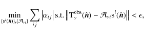
Among the available techniques we choose to use the generalized
morphological component analysis (hereafter GMCA), which is a blind
component separation method. In the GMCA, each observation
![]() is assumed to be the linear combination of
is assumed to be the linear combination of ![]() components
components
![]() so that
so that
|
(15) |
where
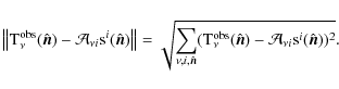
Let
![]() be the set of vectors that forms the dictionary
be the set of vectors that forms the dictionary
![]() .
Let
.
Let
![]() denote the scalar product coefficients between
denote the scalar product coefficients between
![]() and
and
![]() .
When
.
When
![]() is an orthogonal wavelet basis, the following properties hold
is an orthogonal wavelet basis, the following properties hold
| |
= | ||
| = | 1 | ||
| = | 
|
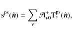
Then GMCA estimates the components
|
(16) |
where
|
(17) |
The GMCA estimates the components
For Planck, the parameter ![]() is chosen to be very small. In that case,
the components
is chosen to be very small. In that case,
the components
![]() are estimated by applying the pseudo-inverse of the
mixing matrix
are estimated by applying the pseudo-inverse of the
mixing matrix
![]() to the observation channels
to the observation channels
![]() :
:
where
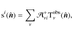
Another important consequence is that these properties give us a conservative method to estimate the
point source residuals remaining within the CMB maps after foreground cleaning, as described below.
Because each source has its own spectral property, component separation techniques fail at disentangling
the point sources emission from the observed maps. As a result, point sources remain mixed with the other
components and the precise amount of the point sources emission by observation channels that has leaked
in each component, is determined by the coefficients of the mixing matrix. More formally, in order to estimate
the point source residuals embedded in the foreground-cleaned CMB maps, quoted
![]() ,
one can apply Eq. (18) to the simulated point sources
in the observation channels
,
one can apply Eq. (18) to the simulated point sources
in the observation channels
![]()
|
(19) |
where the elements
We performed the component separation with the GMCA on Sets I-fg and II-fg, each of 300 simulated patches generated following our idealized Planck sky model and described in the previous Sect. 3.1. As an output of this process, we obtained two sets of 300 foreground-cleaned CMB temperature maps. Note that the GMCA achieves the extraction of the foreground components as well. Unresolved point source residuals are added to each map of these two sets. Below we will refer to the sets of lensed CMB maps with galactic dust, SZ effect and point source residuals after the GMCA component separation as to Sets I- GMCA and II- GMCA respectively.
3.3 CMB lensing reconstruction
Here we apply a discrete version of the quadratic estimator developed by Okamoto & Hu (Eq. (6)) on the different sets of simulated maps previously described, namely Sets I, I- GMCA, II and II- GMCA. We seek to assess the foreground residuals impact on our capability to reconstruct CMB lensing with Planck.
3.3.1 Testing the estimator performances
![\begin{figure}
\par\vfill
\mbox{\includegraphics*[width=5.7cm]{12001fig/12001fi...
...mm}
\includegraphics*[width=6.5cm]{12001fig/12001fig2c} }
\vfill
\end{figure}](/articles/aa/full_html/2010/11/aa12001-09/img112.png)
|
Figure 2:
Impact of the foregrounds residuals on the deflection field reconstruction on
|
| Open with DEXTER | |
First we explicitly give the expression of the discrete quadratic estimator that we derive from Eq. (6):
where
We studied our capability to reconstruct a map of the integrated potential field with the
Planck-HFI idealized simulation, assuming a perfect component separation without any foreground
residuals. We applied the discrete quadratic estimator on the Set I maps (see Sect. 3.1)
to obtain 300 estimates of the same realization of the projected potential field ![]() .
Once stacking these estimates, the final
.
Once stacking these estimates, the final ![]() map is an estimate of the input
map is an estimate of the input ![]() realization.
Following Hu (2001b), we prefer to present our results in terms of the deflection field amplitude
rather than the very smooth gravitational potential field, to highlight the intermediate angular
scales features. Figure 2 shows the input deflection field realization, which was used to
simulate the lensing effect in the Set I maps (on the first panel), as well as its reconstruction with the
quadratic estimator applied on the Set I maps (second panel). Even if the reconstruction noise is visible at
smaller angular scales, the features of the deflection map are well recovered.
realization.
Following Hu (2001b), we prefer to present our results in terms of the deflection field amplitude
rather than the very smooth gravitational potential field, to highlight the intermediate angular
scales features. Figure 2 shows the input deflection field realization, which was used to
simulate the lensing effect in the Set I maps (on the first panel), as well as its reconstruction with the
quadratic estimator applied on the Set I maps (second panel). Even if the reconstruction noise is visible at
smaller angular scales, the features of the deflection map are well recovered.
Characterizing Planck sensitivity to the projected
potential APS requires us to account for both the CMB and the projected
potential field cosmic variances. Thus, we moved on to Set II. As
before we applied the quadratic estimator (Eq. (20)) on the lensed CMB maps to reconstruct
projected potential fields. Averaging over the APS of these individual ![]() field estimates gave
an evaluation of the quadratic estimator variance (as defined in Eq. (11)). The final reconstructed
projected potential APS was obtained by subtracting the noise contributions,
described in Sect. 2, from the variance. The former is related by Eq. (3) to
the deflection APS shown in the Fig. 3. The error bars were estimated as the dispersion
between each individual deflection APS reconstruction. Thus the Set II maps, which are idealized versions
of the Planck-HFI sky assuming a perfect component separation, lead to a good reconstruction of the
deflection APS up to
field estimates gave
an evaluation of the quadratic estimator variance (as defined in Eq. (11)). The final reconstructed
projected potential APS was obtained by subtracting the noise contributions,
described in Sect. 2, from the variance. The former is related by Eq. (3) to
the deflection APS shown in the Fig. 3. The error bars were estimated as the dispersion
between each individual deflection APS reconstruction. Thus the Set II maps, which are idealized versions
of the Planck-HFI sky assuming a perfect component separation, lead to a good reconstruction of the
deflection APS up to
![]() .
The error-bars evaluated here give an upper limit of the
Planck-HFI sensitivity to the deflection APS. As one can see in Fig. 4, they are compatible
with the theoretical 1
.
The error-bars evaluated here give an upper limit of the
Planck-HFI sensitivity to the deflection APS. As one can see in Fig. 4, they are compatible
with the theoretical 1![]() error-bars one can calculate from the Fisher formalism
error-bars one can calculate from the Fisher formalism
where
3.3.2 Impact of the foreground residuals
Here we essentially redo the same analysis, but with the full-simulation pipeline of our Planck-HFI demonstration model. The integrated potential field is extracted from the Sets I- GMCA and II- GMCA described in Sect. 3.2.
First, we aim at developing an intuition for the impact of foreground residuals on the deflection map reconstruction. We used the Set I- GMCA, in which both deflection field and foreground realizations are fixed. As previously, the 300 deflection field estimates reconstructed with the quadratic estimator were stacked to produce a unique reconstructed deflection field shown in Fig. 2. We can see that the recovery of the underlying deflection field is still achieved even with foregrounds emission and after the GMCA. The impact of the foreground residuals is nevertheless visible, mostly at angular scales larger than 2 degrees, whereas the intermediate angular scale features seem more preserved.
For a more quantitative analysis, we moved on to the impact of the foreground residuals on the deflection APS reconstruction. We used the Set II- GMCA (see Sects. 3.1 and 3.2) to ensure that the variances of the CMB, the deflection field and the foregrounds were accounted for. We reconstructed a deflection field estimate from each of the Set II- GMCA maps with the quadratic estimator given in Eq. (20). Finally, we obtained the reconstructed deflection APS from the average variance over these 300 deflection APS estimates as described in Sect. 3.3.1.
![\begin{figure}
\par\resizebox{9cm}{!}{\includegraphics[viewport= 7 0 555 406,clip]{12001fig/12001fig3}}
\end{figure}](/articles/aa/full_html/2010/11/aa12001-09/img134.png)
|
Figure 3:
Deflection APS. Data-points are the binned APS reconstructed from Planck
synthetic lensed CMB maps in two cases: (light blue/grey) the ideal case without any foreground and
(dark blue/black) the case with foreground residuals from the GMCA output CMB maps. The fiducial deflection APS
calculated with CAMB is figured by the (orange/solid) line; the orange/grey data points are the binned deflection APS
estimates on the 300 input deflection field realizations. The horizontal and vertical intervals associated
with the data points represent the averaging multipole bands and the 1 |
| Open with DEXTER | |
The reconstructed binned deflection APS with the evaluated 1![]() errors is
represented in Fig. 3. Figure 4 shows the difference between the
reconstructed and the input deflection APS. First we report that the foreground residuals do
not compromise the Planck-HFI capability to reconstruct the deflection APS - or equivalently
the integrated potential APS. Figure 3 shows that the APS reconstruction is preserved
at the angular scales from L=60 up to L=2600.
In this multipole range, the GMCA algorithm succeeds in letting the
statistical properties of the lensed CMB temperature anisotropies
unchanged, which suggests that this is a well-appropriated component
separation tool for CMB lensing reconstruction. As for the first
multipole bin, we report a 4
errors is
represented in Fig. 3. Figure 4 shows the difference between the
reconstructed and the input deflection APS. First we report that the foreground residuals do
not compromise the Planck-HFI capability to reconstruct the deflection APS - or equivalently
the integrated potential APS. Figure 3 shows that the APS reconstruction is preserved
at the angular scales from L=60 up to L=2600.
In this multipole range, the GMCA algorithm succeeds in letting the
statistical properties of the lensed CMB temperature anisotropies
unchanged, which suggests that this is a well-appropriated component
separation tool for CMB lensing reconstruction. As for the first
multipole bin, we report a 4![]() excess of the deflection signal in the
L=2 to L=60 multipole range. We checked that this bias is linked to the introduction of
the unresolved point source residuals in our simulation pipeline. Interestingly, we found that this excess
originates not in the level of residuals themselves, but mostly in the cutting procedure
excess of the deflection signal in the
L=2 to L=60 multipole range. We checked that this bias is linked to the introduction of
the unresolved point source residuals in our simulation pipeline. Interestingly, we found that this excess
originates not in the level of residuals themselves, but mostly in the cutting procedure![]() we used to extract the set of 300 square maps from our full-sky point source residuals. We postpone a closer
inspection of the low multipole lensing reconstruction behavior to the complete full-sky study
(below in Sect. 4). Apart from the excess signal in the first bin, the impact of the foreground
residuals on the deflection reconstruction is also slightly visible at all angular scales, as
seen in the Fig. 4. If the difference between reconstructed and input APS is still compatible
with zero within the theoretical 1
we used to extract the set of 300 square maps from our full-sky point source residuals. We postpone a closer
inspection of the low multipole lensing reconstruction behavior to the complete full-sky study
(below in Sect. 4). Apart from the excess signal in the first bin, the impact of the foreground
residuals on the deflection reconstruction is also slightly visible at all angular scales, as
seen in the Fig. 4. If the difference between reconstructed and input APS is still compatible
with zero within the theoretical 1![]() errors in the 60 to 2600 multipole range, this residual bias appears
more featured, more oscillating than in the previous no-foreground-case.
errors in the 60 to 2600 multipole range, this residual bias appears
more featured, more oscillating than in the previous no-foreground-case.
![\begin{figure}
\par\resizebox{9cm}{!}{\includegraphics[viewport= 7 0 555 406,clip]{12001fig/12001fig4}}
\end{figure}](/articles/aa/full_html/2010/11/aa12001-09/img135.png)
|
Figure 4:
Residual bias of the deflection APS reconstruction. Data-points figure
the difference between the reconstructed and the input deflection APS
averaging over 300 estimates: in the ideal case in light blue/grey and in the case with foreground residuals in dark blue/black (consistent
with the Fig. 3 caption). The lines show the non-Gaussian noise terms of the
quadratic estimator at the first-order (violet/dashed) and at the second-order (red/long dashed) in
|
| Open with DEXTER | |
To quantify this degradation in the deflection APS reconstruction, we calculated the total error in unit of ![]() ,
defined as
,
defined as
|
(22) |
where
As a final remark we note that because of the first bin excess signal problem, which is linked to the sphere to patches transition, one might prefer a full-sky approach when seeking a precise lensing reconstruction at the higher (L<60) angular scales.
4 Impact of masks on the full-sky lensing reconstruction
4.1 Introduction
From now on, we move to a full-sky analysis of the CMB lensing effect. Some large areas of the map, where the CMB signal is highly dominated by the foreground emission (e.g. the galactic plane, the point source directions), have to be masked out. Cutting to zero introduces some mode-coupling within the CMB observables. As the lensing reconstruction methods rely on the off-diagonal terms of the CMB data covariance matrix, the map-masking yields some artifacts in the projected potential estimate if not accounted for. Several methods have been proposed to treat the masking effect for extracting the lensing potential field from the WMAP data. In Smith et al. (2007), the reconstruction is performed on the least-square estimate of the signal given the all-channels WMAP temperature data, requiring the inversion of the total data covariance matrix (S+N). However, relying at least on the inversion of the noise covariance matrix, such an optimal data filtering approach is very CPU-consuming when applied to the WMAP maps. The Planck-HFI provides 50 Mega pixels maps. Thas is why the previous method to account for the masking will be difficult to extend to Planck. In Hirata et al. (2008), the need for dealing with the noise covariance matrix is avoided by cross-correlating different frequency band maps. However, this method implies that no component separation has been performed on the CMB maps before the lensing extraction. As a result, a lot of non-Gaussianities of foreground emission origin yield some artifact in the projected potential estimate, requiring a challenging post-processing to be corrected out. As previously mentioned, the Planck collaboration devotes considerable effort in the component separation activities, and the currently developed methods have already proved their efficiency (Leach et al. 2008). Moreover, the results we obtained with the demonstration analysis (see Sect. 3) tend to indicate that the lensing reconstruction is still doable after a component separation. Hence we plan to exploit the Planck frequency band maps to clean out the foreground emission before reconstructing the lensing potential rather than using the cross-correlation based lensing estimator. As a consequence, we need an alternative method to solve the masking issue in maps at the Planck resolution. Here we propose to use an inpainting method, assess its impact on the CMB lensing retrieval and check its robustness to the presence of foregrounds residuals within the CMB map.
First, we describe the hypothesis assumed and the tools we use to generate synthetic all-sky lensed temperature maps for Planck. Then we describe our full-sky lensing estimator and test its performances on some Planck-like temperature maps. Finally, we review the inpainting method and conclude in studying the effect of the inpainting on the projected potential APS reconstruction in two cases, first assuming a perfect component separation, then with point source residuals.
4.2 Full-sky simulation
The formalism reviewed in Sect. 2 is almost fully applicable
to the spherical case. In particular the remapping
equation (Eq. (1)) still holds, so that a lensed CMB sphere is given by
where the
The LENSPIX![]() package
described in Lewis (2005) aims at generating a set of lensed CMB
temperature and polarization maps from the analytical auto- and cross-APS of
package
described in Lewis (2005) aims at generating a set of lensed CMB
temperature and polarization maps from the analytical auto- and cross-APS of
![]() ,
the temperature, the E and B polarization modes and the line-of-sight projected
potential respectively. The maps are provided in the
HEALP IX
,
the temperature, the E and B polarization modes and the line-of-sight projected
potential respectively. The maps are provided in the
HEALP IX![]() pixelization scheme (Górski et al. 2005). The CMB lensing simulation is achieved in remapping the anisotropy fields according to Eq. (23) of a higher
resolution map using a bi-cubic interpolation scheme in equi-cylindrical pixels. A lensed temperature
map at the Planck resolution (nside = 2048) can be computed in
about five minutes on a 4-processors machine.
The relative difference between the lensed temperature APS
reconstructed on such a map and the lensed APS analytically obtained with
CAMB
pixelization scheme (Górski et al. 2005). The CMB lensing simulation is achieved in remapping the anisotropy fields according to Eq. (23) of a higher
resolution map using a bi-cubic interpolation scheme in equi-cylindrical pixels. A lensed temperature
map at the Planck resolution (nside = 2048) can be computed in
about five minutes on a 4-processors machine.
The relative difference between the lensed temperature APS
reconstructed on such a map and the lensed APS analytically obtained with
CAMB![]() (Lewis et al. 2000) is below 1% up
to l=2750. Here, to conservatively ensure a relative error below 1%, we choose a multipole cut at
(Lewis et al. 2000) is below 1% up
to l=2750. Here, to conservatively ensure a relative error below 1%, we choose a multipole cut at
![]() .
By its speed and precision quality, LENSPIX is a well-adapted tool for
a CMB lensing analysis with Planck data alone.
.
By its speed and precision quality, LENSPIX is a well-adapted tool for
a CMB lensing analysis with Planck data alone.
We obtained some Planck-HFI synthetic maps as in the flat-sky case (see Sect. 3).
White Gaussian noise realizations and Gaussian beam effect were
added to the lensed temperature maps provided by the LENSPIX code. This
Gaussian noise contribution is fully defined by the all-channels beam-deconvolved APS given by
where
For the lensing reconstruction analysis we prepared two sets of 50 all-sky maps with 1.7 arcmin of angular resolution (the HEALP IX resolution parameter nside = 2048). In each set, maps are the lensed CMB temperature plus the Planck-HFI nominal Gaussian noise.
4.3 Full sky lensing reconstruction
We carried out an integrated potential estimation tool based on the full-sky version of the quadratic estimator derived in Hu (2001a). We closely followed the prescription given in Okamoto & Hu (2003) to build an efficient estimator, so that
where
| |
= | (26) | |
| = | 
|
The covariant derivative operator
Then, extending to the spherical case the calculations reviewed in Sect. 2,
the covariance of the integrated potential field estimator
![]() ,
averaged over
an ensemble of CMB and gravitational potential field realizations, depends on the
potential APS, so that
,
averaged over
an ensemble of CMB and gravitational potential field realizations, depends on the
potential APS, so that
where NL (0), NL (1) and NL (2) are zeroth, first and second order in
Within the framework of Monte-Carlo analysis, we built a projected potential APS estimator so that
![\begin{displaymath}\widehat{C}_L^{~ \phi\phi} ~ = ~ \frac{1}{N} \sum_{i=1}^{N} \...
...^i\vert^2 \right] - (N_L^{~ (0)} + N_L^{~ (1)} + N_L^{~ (2)}),
\end{displaymath}](/articles/aa/full_html/2010/11/aa12001-09/img161.png)
where
![\begin{figure}
\par\vfill
\mbox{\includegraphics*[angle=90,width=8cm]{12001fig/1...
...s*[angle=90,width=8cm]{12001fig/12001fig5d} }
\vfill\vspace*{8mm}
\end{figure}](/articles/aa/full_html/2010/11/aa12001-09/img164.png)
|
Figure 5: All-sky maps in Galactic Mollweide projection. Upper panels: ( left) a Planck-HFI synthetic CMB temperature map in milliKelvin, ( right) the union mask defined in Sect. 4.5. The grey region shows the observed pixels, whereas the rejected ones are in black. Lower panels: left panel shows the restored CMB map obtained by applying the inpainting process (described in Sect. 4.4) on the previous upper-left CMB map masked according to the union mask and the right panel shows the difference between the input (upper-left) CMB map and the restored (lower-left) one. |
| Open with DEXTER | |
Finally, we tested our APS estimator on a set of 10 lensed CMB temperature maps of 50 millions of pixels,
including the nominal Planck noise, generated as described in Sect. 4.2. As in
the flat-sky case, sums in the spherical harmonic space were cut at
![]() .
The results, compiled in the form of an integrated potential APS estimate averaged over the 10 trials
(see Eq. (28)), are shown in the left panels of Fig. 6.
.
The results, compiled in the form of an integrated potential APS estimate averaged over the 10 trials
(see Eq. (28)), are shown in the left panels of Fig. 6.
4.4 Inpainting the mask
We took into account the cutting effect of the temperature map before any lensing reconstruction rather than making any changes in the quadratic estimator (given in Eq. (25)) to account for the mask. This approach was motivated by the high quality and the large frequency coverage of the Planck data, which allow one to reconstruct the CMB temperature map on roughly 90% of the sky. It therefore suggests that a method intended to fill the gap in the map can be applicable.
Several methods, which are referred to as inpainting, were recently developed since the pioneering work of Masnou & Morel (1998). The general purpose of these methods is to restore missing or damaged regions of an image to retrieve the original image as far as possible. For the CMB lensing reconstruction, the ideal inpainting method would lead a restored map with the same statistical properties as the underlying unmasked map. To use a notion briefly mentioned in Sect. 3.2, the masking effect can be thought of as a loss of sparcity in the map representation: the information required to define the map has been spread across the spherical harmonics basis. That is the reason why the inpainting process can also be thought of as a restoration of the CMB temperature field sparcity in a conveniently chosen waveform dictionary.
![\begin{figure}
\par\vfill
\mbox{\includegraphics*[width=8.5cm]{12001fig/12001fi...
...m}
\includegraphics*[width=8.5cm]{12001fig/12001fig6d} }
\vfill
\end{figure}](/articles/aa/full_html/2010/11/aa12001-09/img169.png)
|
Figure 6:
Impact of the masking corrected by an inpainting process. The left panels are for the full-sky
Planck synthetic lensed temperature maps, whereas the right panels compile the results drawn from the masked
lensed temperature maps restored with the inpainting process described in Sect. 4.4.
Upper panels: the reconstructed deflection APS
|
| Open with DEXTER | |
Elad et al. (2005) introduced a sparsity-based
technique to fill in the missing pixels. This method was extended to the sphere in Abrial et al. (2008,2007). In a nutshell, the masked CMB map is modeled as follows:
| (29) |
where
|
(30) |
where
4.5 Effect of inpainting
First we have to choose a realistic mask, which could also be applied to the forthcoming Planck temperature map. However, depending on the details of the component separation pipeline the different methods developed in the Planck consortium (see Leach et al. 2008) yield slightly different masks. Furthermore, the mask size is not a necessary criteria for the final choice of the component separation method that will be selected for the Planck data analysis. We thus adopt a conservative approach, which consists in choosing the union of the masks provided by each of the methods at the time of the component separation Planck working group second challenge (Leach et al. 2008). This mask, hereafter referred to as the union mask, rejects about 11% of the sky, as shown in Fig. 5.
Then the 10 Planck-like lensed CMB temperature maps we generated (see Sect. 4.2) were masked according to the union mask and then restored by applying the inpainting
method described in Abrial et al. (2008). From each of these mask-corrected maps we extracted a projected
potential field using the quadratic estimator of Eq. (25). As previously, the results
were compiled in the form of the average projected potential APS
![]() following Eq. (28). The reconstructed deflection APS,
given by
following Eq. (28). The reconstructed deflection APS,
given by
![]() ,
as well as the bias between
estimated and fiducial deflection APS
,
as well as the bias between
estimated and fiducial deflection APS
![]() are shown in the right panels of Fig. 6.
are shown in the right panels of Fig. 6.
We found that the mask corrected by the inpainting results in a marginal increase (![]() 4%) of the 1
4%) of the 1![]() errors on the estimated deflection APS (hence on the projected potential APS). Masking and inpainting causes
an increase of the reconstructed APS bias
errors on the estimated deflection APS (hence on the projected potential APS). Masking and inpainting causes
an increase of the reconstructed APS bias
![]() arising mostly at
large angular scale corresponding to multipole L<300. However, this bias is weaker than the
sub-dominant second-order in
arising mostly at
large angular scale corresponding to multipole L<300. However, this bias is weaker than the
sub-dominant second-order in
![]() non-Gaussian bias. Figure 6 shows a clear
increase of power in the very first multipole band (2<l<10). In this multipole range, Planck
is not expected to achieve a good reconstruction of the potential APS (Hu & Okamoto 2002). From the multipole
L=300 up to L=2600, the bias stays below the first-order in
non-Gaussian bias. Figure 6 shows a clear
increase of power in the very first multipole band (2<l<10). In this multipole range, Planck
is not expected to achieve a good reconstruction of the potential APS (Hu & Okamoto 2002). From the multipole
L=300 up to L=2600, the bias stays below the first-order in
![]() non-Gaussian bias and is
compatible with the theoretical 1
non-Gaussian bias and is
compatible with the theoretical 1![]() errors expected for the quadratic estimator. From fully
controlling the inpainting impact, one might want to push further the study by analytically calculating
or Monte-Carlo estimating the mask induced bias. However, it is not mandatory for
reconstructing the projected potential APS with Planck. The masking effect, once corrected by
inpainting, becomes a sub-dominant systematic effect that can be safety neglected.
errors expected for the quadratic estimator. From fully
controlling the inpainting impact, one might want to push further the study by analytically calculating
or Monte-Carlo estimating the mask induced bias. However, it is not mandatory for
reconstructing the projected potential APS with Planck. The masking effect, once corrected by
inpainting, becomes a sub-dominant systematic effect that can be safety neglected.
4.6 Robustness against the unresolved point sources
Up to now, we handled two important issues linked to the presence of foreground emissions in the observation maps independently, the impact of the foreground residuals after component separation with GMCA in Sect. 3.3 and the impact of the masking corrected with the inpainting method in the previous subsection (Sect. 4.5). We found that none of them compromises our ability to reconstruct the deflection APS. In a more realistic approach, these two issues should be handled together, as the inpainting process is intended to be applied on a CMB map contaminated by foreground residuals. Foreground residuals are likely to harden the inpainting process and consequently degrade the CMB lensing recovery. Here we assess the robustness of the deflection reconstruction on masked and inpainted CMB maps when adding infra-red point source residuals. This choice was made for two reasons. The point source residuals after component separation are a well-known matter of concern in any CMB non-Gaussianities analysis and the emission of the infra-red sources population is one of the major foreground contaminants at the Planck-HFI observation channels.
We used the full-sky map of infra-red point source residuals after a component separation with the GMCA, which we had estimated in Sect. 3.2. Thess point source residuals were added to the 10 synthetic Planck-lensed CMB temperature maps described in Sect. 4.2. Then we repeated the same analysis as previously in Sect. 4.5: the union mask was applied to the maps, cutting out the brightest infra-red sources, which were detected during the Component Separation Planck working group second challenge (Leach et al. 2008). The 10 masked maps were restored with the inpainting method before being ingested in the full-sky quadratic estimator of the projected potential field. The results of the whole analysis are presented in the form of the average reconstructed deflection APS and bias in Fig. 7.
We found that the inpainting performances were only marginally degraded (at ![]()
![]() level) by the
point source residuals within the CMB maps, and this degradation occured mainly at the two multipole
extremes. At the lower multipoles (L<30), the APS deflection reconstruction suffers from a 1
level) by the
point source residuals within the CMB maps, and this degradation occured mainly at the two multipole
extremes. At the lower multipoles (L<30), the APS deflection reconstruction suffers from a 1![]() increase of the bias, whereas at the higher multipoles, only the error bars increase. We conclude that the inpainting
method succeeds in keeping the statistical properties of the CMB map unchanged even with highly non-Gaussian foreground
residuals and is a qualified method to handle the masking issue when
seeking a CMB lensing recovery. In addition, the results compiled in the Fig. 7 give
the total impact of point sources on the deflection reconstruction, as they account for both the masking
of the bright detected sources and the unresolved residuals. We report that point sources are responsible for
a total
increase of the bias, whereas at the higher multipoles, only the error bars increase. We conclude that the inpainting
method succeeds in keeping the statistical properties of the CMB map unchanged even with highly non-Gaussian foreground
residuals and is a qualified method to handle the masking issue when
seeking a CMB lensing recovery. In addition, the results compiled in the Fig. 7 give
the total impact of point sources on the deflection reconstruction, as they account for both the masking
of the bright detected sources and the unresolved residuals. We report that point sources are responsible for
a total ![]() increase of the
increase of the ![]() errors on the reconstructed APS deflection, mainly induced by the
unresolved residuals. As a summary, the major nuisance of point sources is related to the masking of the
bright ones, which tend to increase the bias on the reconstructed deflection APS, whereas the unresolved
residuals result mainly in an increase of the errors on the deflection retrieval.
errors on the reconstructed APS deflection, mainly induced by the
unresolved residuals. As a summary, the major nuisance of point sources is related to the masking of the
bright ones, which tend to increase the bias on the reconstructed deflection APS, whereas the unresolved
residuals result mainly in an increase of the errors on the deflection retrieval.
![\begin{figure}
\par\vfill
\includegraphics*[width=9cm]{12001fig/12001fig7a} \vfill
\includegraphics*[width=9cm]{12001fig/12001fig7b} \vfill
\end{figure}](/articles/aa/full_html/2010/11/aa12001-09/img187.png)
|
Figure 7: Robustness of the inpainting to the unresolved point sources. The upper panel shows the reconstructed deflection APS, whereas the lower panel the bias on the deflection APS reconstruction. The (dark blue/black) data points show the result of the full-sky quadratic estimation on the set of lensed CMB maps with point source residuals, which were masked and then restored with the inpainting technique, as described in Sect. 4.6. For comparison the results obtained in Sect. 4.5 in the case without any sources residuals, are shown here as (light blue/grey) crosses. The fiducial analytical deflection APS as well as the total reconstruction noise and the two APS bias are shown following the same representation code as in Fig. 6, and horizontal and vertical intervals have the same meaning as described in the Fig. 6 caption. For clarity only the band power reconstructed APS and APS bias are represented, and the theoretical error bars by multipole bins are not shown. |
| Open with DEXTER | |
Conclusions
The High Frequency Instrument (HFI) of the Planck satellite, which was launched on the 14th of May 2009, has the sensitivity and the angular resolution required to allow a reconstruction of the CMB lensing using the temperature anisotropies map alone. The pioneer works to put evidence of the CMB lensing within the WMAP data are not directly applicable or not well-optimized to the Planck data. First, one might want to take advantage of the efficient component separation algorithms developed for Planck before applying a CMB lensing estimator rather than to correct the lensing reconstruction from the bias due to the foreground emission afterward. Second, we need an efficient and manageable method to take into account the sky cutting within the 50 Mega-pixels maps provided by Planck. In addition, the CMB lensing is related to another imminent problem: characterizing the non-Gaussianities of the temperature anisotropies (primordial non-Gaussianities, cosmic string, etc.).
We implemented both the flat-sky and the all-sky versions of the quadratic estimator of the
projected potential field described in Okamoto & Hu (2003); Hu (2001b) to apply them to Planck
synthetic temperature maps. First, we prepared a demonstration model within the
flat-sky approximation, which consists in running the GMCA,
a component separation method described in Bobin et al. (2008), on Planck frequency channel synthetics
maps, containing the lensed CMB temperature, the Planck nominal instrumental effects (modeled by a
white Gaussian noise and a Gaussian beam) and the three dominant foreground emissions at the
Planck-HFI observation frequencies, namely the SZ effect, the galactic dust and the infra-red point
sources. We performed a Monte-Carlo analysis to quantify the impact of the foreground residuals after
the GMCA on the projected potential field and APS reconstructions. Then we moved on to the full-sky
case, using the LensPix algorithm (Lewis 2005) to generate lensed CMB temperature
maps at the Planck resolution. We performed a Monte-Carlo analysis to tackle
the masking issue; we used the inpainting method described in Abrial et al. (2008) to restore
the Planck synthetic temperature maps, masked according to a realistic cut out of 11![]() of the sky,
accounting for the bright detected point sources. By applying the projected potential quadratic
estimator on these restored maps, we studied the impact of the inpainting of the mask on the
Planck sensitivity to the projected potential APS. Finally, we assessed the total impact
of the point sources emission, in confronting the inpainting method with the unresolved point source
residuals.
of the sky,
accounting for the bright detected point sources. By applying the projected potential quadratic
estimator on these restored maps, we studied the impact of the inpainting of the mask on the
Planck sensitivity to the projected potential APS. Finally, we assessed the total impact
of the point sources emission, in confronting the inpainting method with the unresolved point source
residuals.
Results
- 1.
- Within our flat-sky demonstration model, we found that the reconstruction of the
projected potential field is still feasibleafter a component separation with the GMCA. More
quantitatively, the foreground residuals in the GMCA output CMB maps lead to a
 increase
of the 1
increase
of the 1 errors on the projected potential APS reconstruction when applying the quadratic
estimator. The GMCA process results in an increase of the dispersion of the projected potential APS
reconstruction, but this dispersion remains within the theoretical 1
errors at all
angular scales but the L<60 multipoles, in which the flat-sky analysis is expected to show some
limitations anyway. A study like this, dealing with the impact of a component separation process on the CMB
lensing reconstruction, has never been performed before. Our results allow us to assess that applying
a component separation algorithm on the frequency channel CMB maps before any lensing estimation is
a well-adapted strategy for the projected potential reconstruction within Planck.
errors on the projected potential APS reconstruction when applying the quadratic
estimator. The GMCA process results in an increase of the dispersion of the projected potential APS
reconstruction, but this dispersion remains within the theoretical 1
errors at all
angular scales but the L<60 multipoles, in which the flat-sky analysis is expected to show some
limitations anyway. A study like this, dealing with the impact of a component separation process on the CMB
lensing reconstruction, has never been performed before. Our results allow us to assess that applying
a component separation algorithm on the frequency channel CMB maps before any lensing estimation is
a well-adapted strategy for the projected potential reconstruction within Planck.
- 2.
- For the full-sky reconstruction of the projected potential APS with Planck, we
report that a realistic 11
 of the sky mask, applied on some Planck-nominal lensed CMB
temperature maps, has a negligible impact on the CMB lensing signal retrieval process, whenever
it has been corrected by the inpainting method of Abrial et al. (2008) beforehand. More
precisely, the bias on the estimated projected potential APS induced by the mask after inpainting is
always either compatible with the theoretical
of the sky mask, applied on some Planck-nominal lensed CMB
temperature maps, has a negligible impact on the CMB lensing signal retrieval process, whenever
it has been corrected by the inpainting method of Abrial et al. (2008) beforehand. More
precisely, the bias on the estimated projected potential APS induced by the mask after inpainting is
always either compatible with the theoretical  errors (from l=300 up to l=2600) or
weaker than the second-order in
errors (from l=300 up to l=2600) or
weaker than the second-order in
 non-Gaussian bias (in the l<300 range). The major
impact of the inpainting correction on the projected potential APS arises at the larger angular
scales (2<l<10), which are not expected to be well-reconstructed with Planck. In addition,
these results did not significantly change after the introduction of unresolved point source residuals.
When treating the point sources emission in a comprehensive way, we report a
non-Gaussian bias (in the l<300 range). The major
impact of the inpainting correction on the projected potential APS arises at the larger angular
scales (2<l<10), which are not expected to be well-reconstructed with Planck. In addition,
these results did not significantly change after the introduction of unresolved point source residuals.
When treating the point sources emission in a comprehensive way, we report a  increase of the
errors on the reconstructed deflection APS on average, resulting mainly
from the unresolved point source residuals, whereas the level of bias
is marginally increased at low multipoles. We conclude that applying
the inpainting method of Abrial et al. (2008) beforehand is a good strategy to take into account the masking issue when seeking to reconstruct the projected potential with Planck.
increase of the
errors on the reconstructed deflection APS on average, resulting mainly
from the unresolved point source residuals, whereas the level of bias
is marginally increased at low multipoles. We conclude that applying
the inpainting method of Abrial et al. (2008) beforehand is a good strategy to take into account the masking issue when seeking to reconstruct the projected potential with Planck.
Perspectives
Our results on the CMB lensing reconstruction are the first step to develop a complete analysis chain dedicated to the projected potential APS reconstruction with the Planck data. This CMB lensing reconstruction pipeline should involve a component separation and a bright point sources detection followed by an algorithm to correct from the mask (e.g. the inpainting method) before applying a quadratic estimator of the projected potential field on the resulting CMB temperature map.We plan to simultaneously work on both the flat-sky and the full-sky reconstruction tools. The flat-sky tools will allow us to perform a multi-patches CMB lensing reconstruction in cutting several hundred patches out of the most foreground-cleaned region of the full-sky map. Using such a method requires a quantitative study of the impact of the sphere-to-plan projection and the sharp edge cut effects beforehand. As a first task, we will test whether our results concerning the feasibility of reconstructing the CMB lensing after a component separation and after an inpainting of the mask still hold when dealing with the fully realistic Planck simulation (including e.g. a non-axisymmetric beam, inhomogeneous noise and correlated foreground emissions). As long as we can demonstrate we have sufficient control on the systematics, we will be ready to measure the projected potential APS with Planck alone. This additional cosmological observable is expected to enlarge the investigation field accessible to the Planck mission from the primordial Universe to us.
AcknowledgementsWe warmly thank Duncan Hanson for providing us the second-order non-Gaussian noise term biasing the projected potential APS estimation and for helpful discussions. We also thank Martin Reinecke for his help on the HEALPix package use. We acknowledge use of the CAMB, LENSPix, HEALPix-Cxx and MRS packages. This work was partially supported by the French National Agency for Research (ANR-05-BLAN-0289-01 and ANR-08-EMER-009-01).
References
- Abrial, P., Moudden, Y., Starck, J., et al. 2007, J. Fourier Analysis and Applications, 13, 729 [CrossRef] [Google Scholar]
- Abrial, P., Moudden, Y., Starck, J.-L., et al. 2008, Statistical Methodology, 5, 289 [Google Scholar]
- Aghanim, N., & Forni, O. 1999, A&A, 347, 409 [NASA ADS] [Google Scholar]
- Amblard, A., Vale, C., & White, M. 2004, New Astron., 9, 687 [NASA ADS] [CrossRef] [Google Scholar]
- Argüeso, F., González-Nuevo, J., & Toffolatti, L. 2003, ApJ, 598, 86 [NASA ADS] [CrossRef] [Google Scholar]
- Babich, D., & Pierpaoli, E. 2008, Phys. Rev. D, 77, 123011 [NASA ADS] [CrossRef] [Google Scholar]
- Barreiro, R. B., Martínez-González, E., Vielva, P., & Hobson, M. P. 2006, MNRAS, 368, 226 [NASA ADS] [Google Scholar]
- Bernardeau, F. 1997, A&A, 324, 15 [NASA ADS] [Google Scholar]
- Blanchard, A., & Schneider, J. 1987, A&A, 184, 1 [NASA ADS] [Google Scholar]
- Bobin, J., Moudden, Y., Starck, J.-L., Fadili, J., & Aghanim, N. 2008, Statist. Methodol., 5, 307 [NASA ADS] [CrossRef] [Google Scholar]
- Challinor, A., & Lewis, A. 2005, Phys. Rev. D, 71, 103010 [NASA ADS] [CrossRef] [Google Scholar]
- Delabrouille, J., Melin, J.-B., & Bartlett, J. G. 2002, in AMiBA 2001: High-Z Clusters, Missing Baryons, and CMB Polarization, ASP Conf. Ser., 257, 81 [Google Scholar]
- Delabrouille, J., Cardoso, J.-F., & Patanchon, G. 2003, MNRAS, 346, 1089 [NASA ADS] [CrossRef] [Google Scholar]
- Elad, M., & Starck, J.-L., Querre, P., & Donoho, D. 2005, Applied and Computational Harmonic Analysis, 19, 340 [CrossRef] [Google Scholar]
- Górski, K. M., Hivon, E., Banday, A. J., et al. 2005, ApJ, 622, 759 [NASA ADS] [CrossRef] [Google Scholar]
- Granato, G. L., De Zotti, G., Silva, L., Bressan, A., & Danese, L. 2004, ApJ, 600, 580 [Google Scholar]
- Guzik, J., Seljak, U., & Zaldarriaga, M. 2000, Phys. Rev. D, 62, 043517 [NASA ADS] [CrossRef] [Google Scholar]
- Hanson, D., Challinor, A., Efstathiou, G., & Bielewicz, P. 2010,[arXiv:1008.4403] [Google Scholar]
- Hirata, C. M., & Seljak, U. 2003a, Phys. Rev. D, 67, 043001 [NASA ADS] [CrossRef] [Google Scholar]
- Hirata, C. M., & Seljak, U. 2003b, Phys. Rev. D, 68, 083002 [NASA ADS] [CrossRef] [Google Scholar]
- Hirata, C. M., Ho, S., Padmanabhan, N., Seljak, U., & Bahcall, N. 2008, Phys. Rev. D, 78, 043520 [NASA ADS] [CrossRef] [Google Scholar]
- Hu, W. 2000, Phys. Rev. D, 62, 043007 [NASA ADS] [CrossRef] [Google Scholar]
- Hu, W. 2001a, Phys. Rev. D, 64, 083005 [NASA ADS] [CrossRef] [Google Scholar]
- Hu, W. 2001b, ApJ, 557, L79 [NASA ADS] [CrossRef] [Google Scholar]
- Hu, W. 2002, Phys. Rev. D, 65, 023003 [NASA ADS] [CrossRef] [Google Scholar]
- Hu, W., & Okamoto, T. 2002, ApJ, 574, 566 [Google Scholar]
- Kamionkowski, M., Kosowsky, A., & Stebbins, A. 1997, Phys. Rev. Lett., 78, 2058 [NASA ADS] [CrossRef] [Google Scholar]
- Kaplinghat, M., Knox, L., & Song, Y.-S. 2003, Phys. Rev. Lett., 91, 241301 [NASA ADS] [CrossRef] [PubMed] [Google Scholar]
- Kesden, M., Cooray, A., & Kamionkowski, M. 2003, Phys. Rev. D, 67, 123507 [NASA ADS] [CrossRef] [Google Scholar]
- Knox, L., & Song, Y.-S. 2002, Phys. Rev. Lett., 89, 011303 [NASA ADS] [CrossRef] [PubMed] [Google Scholar]
- Komatsu, E. 2002, PhD thesis, Tohoku University [Google Scholar]
- Leach, S. M., Cardoso, J., Baccigalupi, C., et al. 2008, A&A, 491, 597 [NASA ADS] [CrossRef] [EDP Sciences] [Google Scholar]
- Lesgourgues, J., Perotto, L., Pastor, S., & Piat, M. 2006, Phys. Rev. D, 73, 045021 [NASA ADS] [CrossRef] [Google Scholar]
- Lewis, A. 2005, Phys. Rev. D, 71, 083008 [NASA ADS] [CrossRef] [Google Scholar]
- Lewis, A., & Challinor, A. 2006, Phys. Rep., 429, 1 [Google Scholar]
- Lewis, A., Challinor, A., & Lasenby, A. 2000, ApJ, 538, 473 [NASA ADS] [CrossRef] [Google Scholar]
- Masnou, S., & Morel, J.-M. 1998, in ICIP, ed. IEEE, 3, 259 [Google Scholar]
- Okamoto, T., & Hu, W. 2003, Phys. Rev. D, 67, 083002 [NASA ADS] [CrossRef] [Google Scholar]
- Park, S. K., & Schowengerdt, R. A. 1983, Computer Graphics Image Processing, 23, 258 [Google Scholar]
- Perotto, L., Lesgourgues, J., Hannestad, S., Tu, H., & Y Y Wong, Y. 2006, J. Cosmology and Astro-Particle Physics, 10, 13 [Google Scholar]
- Riquelme, M. A., & Spergel, D. N. 2007, ApJ, 661, 672 [NASA ADS] [CrossRef] [Google Scholar]
- Seljak, U., & Hirata, C. M. 2004, Phys. Rev. D, 69, 043005 [NASA ADS] [CrossRef] [Google Scholar]
- Seljak, U. & Zaldarriaga, M. 1997, Phys. Rev. Lett., 78, 2054 [NASA ADS] [CrossRef] [Google Scholar]
- Serjeant, S., & Harrison, D. 2005, MNRAS, 356, 192 [NASA ADS] [CrossRef] [Google Scholar]
- Smith, K. M., Zahn, O., & Doré, O. 2007, Phys. Rev. D, 76, 043510 [NASA ADS] [CrossRef] [Google Scholar]
- Su, M., & Yadav, A. P. S.and Zaldarriaga, M. 2009, Phys. Rev. D, 79, 123002 [NASA ADS] [CrossRef] [Google Scholar]
- Sunyaev, R. A., & Zeldovich, Y. B. 1970, Comments on Astrophysics and Space Physics, 2, 66 [Google Scholar]
- Takada, M., & Futamase, T. 2001, ApJ, 546, 620 [NASA ADS] [CrossRef] [Google Scholar]
- Tauber, J. A. 2006, in The Many Scales in the Universe: JENAM 2004 Astrophysics Reviews, ed. J. C. Del Toro Iniesta, E. J. Alfaro, J. G. Gorgas, E. Salvador-Sole, & H. Butcher, 35 [Google Scholar]
- The Planck Consortia 2005, Planck: the scientific programme, ESA-SCI(2006)1 (European Space Agency), [arXiv:astro-ph/0604069] [Google Scholar]
- Zaldarriaga, M. 2000, Phys. Rev. D, 62, 063510 [NASA ADS] [CrossRef] [Google Scholar]
- Zaldarriaga, M., & Seljak, U. 1998, Phys. Rev. D, 58, 023003 [NASA ADS] [CrossRef] [Google Scholar]
Footnotes
- ...Planck
![[*]](/icons/foot_motif.png)
- http://www.rssd.esa.int/index.php?project=PLANCK&page=index
- ... potential
- A priori, the remapping function should depend not only on a convergence field but also on a rotation field, so that the deflection angle is not purely gradient but has a rotational contribution. However, Hirata & Seljak (2003b) have shown that the rotation field effect will be negligible for the next generation of CMB experiments.
- ... CAMB
- Web site: http://camb.info/
- ... procedure
- The cutting procedure involves a sphere-to-plan projection, an apodization and a fit of the Fourier coefficients of the square map. From the tests we run (not presented here), the apodization appears to have the most harmful impact on the high angular scale deflection reconstruction. A complete study of the impact of the sphere to patches transition will be the subject of a companion paper.
- ... LENSPIX
- http://cosmologist.info/lenspix/
- ... IX
- The acronym for ``Hierarchical Equal Area isoLatitude Pixelization'' of a sphere (see http://healpix.jpl.nasa.gov/index.shtml).
- ... CAMB
- The ``Code for Anisotropies in the Microwave Background'' is a so-called Boltzmann's code described at http://camb.info/
- ... package
- http://jstarck.free.fr/mrs.html
All Tables
Table 1:
Instrumental characteristics of Planck-HFI
![]() .
.
All Figures
|
|
Figure 1: CMB temperature APS. The red/black (respectively green/grey) line is the lensed (respectively unlensed) temperature APS calculated with the public Boltzmann code CAMB (Challinor & Lewis 2005; Lewis et al. 2000). The blue/black data-points are the mean of the binned power spectrum reconstructed on 500 simulated lensed temperature maps. The error-bars are given by the variance of the 500 APS estimates. |
| Open with DEXTER | |
| In the text | |
|
|
Figure 2:
Impact of the foregrounds residuals on the deflection field reconstruction on
|
| Open with DEXTER | |
| In the text | |
|
|
Figure 3:
Deflection APS. Data-points are the binned APS reconstructed from Planck
synthetic lensed CMB maps in two cases: (light blue/grey) the ideal case without any foreground and
(dark blue/black) the case with foreground residuals from the GMCA output CMB maps. The fiducial deflection APS
calculated with CAMB is figured by the (orange/solid) line; the orange/grey data points are the binned deflection APS
estimates on the 300 input deflection field realizations. The horizontal and vertical intervals associated
with the data points represent the averaging multipole bands and the 1 |
| Open with DEXTER | |
| In the text | |
|
|
Figure 4:
Residual bias of the deflection APS reconstruction. Data-points figure
the difference between the reconstructed and the input deflection APS
averaging over 300 estimates: in the ideal case in light blue/grey and in the case with foreground residuals in dark blue/black (consistent
with the Fig. 3 caption). The lines show the non-Gaussian noise terms of the
quadratic estimator at the first-order (violet/dashed) and at the second-order (red/long dashed) in
|
| Open with DEXTER | |
| In the text | |
|
|
Figure 5: All-sky maps in Galactic Mollweide projection. Upper panels: ( left) a Planck-HFI synthetic CMB temperature map in milliKelvin, ( right) the union mask defined in Sect. 4.5. The grey region shows the observed pixels, whereas the rejected ones are in black. Lower panels: left panel shows the restored CMB map obtained by applying the inpainting process (described in Sect. 4.4) on the previous upper-left CMB map masked according to the union mask and the right panel shows the difference between the input (upper-left) CMB map and the restored (lower-left) one. |
| Open with DEXTER | |
| In the text | |
|
|
Figure 6:
Impact of the masking corrected by an inpainting process. The left panels are for the full-sky
Planck synthetic lensed temperature maps, whereas the right panels compile the results drawn from the masked
lensed temperature maps restored with the inpainting process described in Sect. 4.4.
Upper panels: the reconstructed deflection APS
|
| Open with DEXTER | |
| In the text | |
|
|
Figure 7: Robustness of the inpainting to the unresolved point sources. The upper panel shows the reconstructed deflection APS, whereas the lower panel the bias on the deflection APS reconstruction. The (dark blue/black) data points show the result of the full-sky quadratic estimation on the set of lensed CMB maps with point source residuals, which were masked and then restored with the inpainting technique, as described in Sect. 4.6. For comparison the results obtained in Sect. 4.5 in the case without any sources residuals, are shown here as (light blue/grey) crosses. The fiducial analytical deflection APS as well as the total reconstruction noise and the two APS bias are shown following the same representation code as in Fig. 6, and horizontal and vertical intervals have the same meaning as described in the Fig. 6 caption. For clarity only the band power reconstructed APS and APS bias are represented, and the theoretical error bars by multipole bins are not shown. |
| Open with DEXTER | |
| In the text | |
Copyright ESO 2010
Current usage metrics show cumulative count of Article Views (full-text article views including HTML views, PDF and ePub downloads, according to the available data) and Abstracts Views on Vision4Press platform.
Data correspond to usage on the plateform after 2015. The current usage metrics is available 48-96 hours after online publication and is updated daily on week days.
Initial download of the metrics may take a while.