| Issue |
A&A
Volume 518, July-August 2010
Herschel: the first science highlights
|
|
|---|---|---|
| Article Number | A31 | |
| Number of page(s) | 12 | |
| Section | Interstellar and circumstellar matter | |
| DOI | https://doi.org/10.1051/0004-6361/200913962 | |
| Published online | 27 August 2010 | |
Spatial distribution of interstellar dust in the Sun's vicinity
Comparison with neutral sodium-bearing gas![[*]](/icons/foot_motif.png)
J.-L. Vergely1 - B. Valette2 - R. Lallement3 - S. Raimond3
1 - ACRI-ST, 260 route du Pin Montard, Sophia Antipolis, France
2 -
Université de Savoie, LGIT-Savoie, 73376 Le-Bourget-du-Lac,
France
3 -
Université Versailles-St Quentin, LATMOS-IPSL, 11 Bd D'Alembert, 78280 Guyancourt, France
Received 23 December 2009 / Accepted 4 March 2010
Abstract
Aims. 3D tomography of the interstellar dust and gas may be
useful in many respects, from the physical and chemical evolution of
the interstellar medium itself to foreground decontamination of the
cosmic microwave background, or various studies of the environments of
specific objects. However, while spectral data cubes of the galactic
emission become increasingly precise, the information on the distance
to the emitting regions has not progressed as well and relies
essentially on the galactic rotation curve. Our goal here is to bring
more precise information on the distance to nearby interstellar dust
and gas clouds within 250 pc.
Methods. We apply the best available calibration methods to a
carefully screened set of stellar Strömgren photometry data for targets
possessing a Hipparcos parallax and spectral type classification. We
combine the derived interstellar extinctions and the parallax distances
for about 6000 stars to build a 3D tomography of the local
dust. We use an inversion method based on a regularized Bayesian
approach and a least squares criterion, optimized for this specific
data set. We apply the same inversion technique to a totally
independent set of neutral sodium absorption data available for about
1700 target stars.
Results. We obtain 3D maps of the opacity and the distance to
the main dust-bearing clouds within 250 pc and identify in those
maps well-known dark clouds and high galactic more diffuse entities. We
calculate the integrated extinction between the Sun and the cube
boundary and compare this with the total galactic extinction derived
from infrared 2D maps. The two quantities reach similar values at
high latitudes, as expected if the local dust content is
satisfyingly reproduced and the dust is closer than 250 pc. Those
maps show a larger high latitude dust opacity in the North compared to
the South, reinforcing earlier evidences. Interestingly the gas maps do
not show the same asymmetry, suggesting a polar asymmetry of the dust
to gas ratio at small distances. We compare the opacity distribution
with the 3D distribution of interstellar neutral sodium resulting
from the inversion of sodium columns. We discuss the similarities and
discrepancies and the influence of data set limitations. Finally we
discuss the potential improvements of those 3D maps.
Key words: ISM: clouds - dust, extinction - local insterstellar matter
1 Introduction
The 3D representation of the local interstellar medium (ISM) is an important challenge from various perspectives. In the most direct way it allows a better modelling of the ISM. The ability to localize masses of gas and dust, combined with information on the ionization state, the temperature and the kinematics helps to understand the chemical and physical evolution of the different gas components in relation to their history and the surrounding ionizing radiation from hot stars, as well as the dust-gas relationships and the dust processing (Cox 2005; Draine 2003).
In a more indirect way, the 3D ISM structure becomes increasingly useful as an ingredient to the foreground contamination of the cosmic microwave background because the local distribution of the gas influences the interstellar radiation field, which in turn influences the dust temperature and infrared-millimetric emission. The 3D distribution of the local ISM is also governing a significant fraction of the diffuse gamma-ray background and is one of the ingredients of the models developed in the context of the Fermi satellite.
In a very different way, the knowledge of the 3D properties of the local ISM may be useful in various other studies because it provides the environmental context of astrophysical objects, allows a correction of the extinction according to the distance and the direction, allows to disentangle spectral lines in absorption related to the object itself or to the foreground, or provides a tool for the estimate of the propagation of energetic particles. The list of topics is too long to be detailed here.
Recent work on the 3D global structure and kinematics of the local ISM or on specific nearby ISM structures has been done using absorption lines in the UV (e.g. Lallement et al. 1995; Redfield & Linsky 2008; Welsh & Lallement 2005) and the strong NaI and CaII interstellar in the visible (e.g. Genova & Beckman 2003; Snow et al. 2008). A number of works have combined emission data and neutral sodium absorption to attribute a distance to specific features seen in radio or IR (e.g. Lilienthal et al. 1992; Corradi et al. 2004; Meyer et al. 2006), making use essentially of Hipparcos parallaxes (Perryman et al. 1997). Neutral species like NaI trace low temperature regions, i.e. dense atomic gas clouds and molecular clouds, while ionized calcium is a tracer of both dense regions (with the exception of the fully neutral cores) and warm diffuse gas, partially ionized (see Welty et al. 1996, for more details). Note that the known existence of different typical sizes linked to the different types of gas, from parsecs for molecular clouds to tens of parsecs for atomic and diffuse clouds, has influenced our choice of correlation lengths for the inversion described in Sect. 4. In parallel, Strömgren photometry has been used in combination with parallaxes for distance estimates of a number of features (e.g. Reis & Corradi 2008; Knude & Høg 1998, 1999)
It is known for a long time from both absorption data and diffuse soft X-ray background detection that the Sun is embedded in a relatively empty cavity, the Local Bubble (LB), mostly devoid of dense clouds (Frisch & York 1983; Sfeir et al. 1999). Within this local cavity reside essentially tenuous diffuse clouds like the clouds that make part of the so-called Local Fluff within 20 pc from the Sun. The interpretation of the soft X-ray background data suggests that the cavity is filled by one million K gas (Snowden et al. 1990). The cavity is delimited by dense clouds whose distances range from 40 to 180 parsecs, and neighboring cavities are distributed all around. This ``cellular'' structure of hot bubbles separated by high density and relatively compact regions including molecular dust clouds is totally expected from the permanent ISM recycling that shapes it: stellar winds and supernova explosions inflate hot ``bubbles'' within the dense gas and maintain these high contrasts (Cox & Reynolds 1987; De Avillez & Breitschwerdt 2004). There is very probably a strong link between the strong winds having inflated the cavity and the surrounding so-called Gould's Belt, an expanding elliptical ring of star-forming regions (see Perrot & Grenier 2003). Several questions remain however about the local ISM and Local Bubble. The embedded clouds are ionized by the early-type stars, but their measured ionization state, especially the ionization of helium, requires an additional harder radiation, which is supposed to be generated within semi-hot conductive interfaces between clouds and hot gas (e.g. Slavin 1989). The distribution of the corresponding semi-hot or hot gas ions however is not in fully satisfying agreement with this scenario (Welsh & Lallement 2005; Savage & Lehner 2006; Knauth et al. 2003). On the other hand the more recent discovery of solar wind charge-transfer X-ray emission (Cox 1998; Cravens 2000) has also complicated the picture because this diffuse emission, which mimics one million K thermal emission, is as intense as the observed background in a number of directions (e.g. Koutroumpa et al. 2009). Decreasing the hot gas pressure significantly would have the positive effect of suppressing the strong difference from the pressure measured within the diffuse clouds and the local cloud (Jenkins 2009).
From 3D gas and dust mapping one can expect significant progresses on these topics, the ``Local Bubble'' wall location and the X-ray emission source regions, some hints about the local bubble formation and the link between the local bubble and surrounding bubbles and more generally a better understanding of the multi-phase structure and the interaction between the different phases of the ISM. One can also expect the determination of the star-forming regions and estimates of the cloud masses. Last but not least, it should help to shed light on the surprisingly high deuterium abundance in the local ISM (Linsky et al. 2006), now largely recognized to be related to a very large extent to dust evaporation from grains (Draine 2004). The unambiguous correlation between refractory metals and deuterium abundances in the gas (Lallement et al. 2008) as well as the peculiar distribution of the deuterium enhancements with respect to the Gould belt (Lallement 2009) suggest a scenario for the formation of the belt with an important role of dust and dust-gas processes.
The first computed tomography of the local ISM from Vergely et al. (2001) used neutral sodium absorption data combined with Hipparcos stellar parallaxes (Perryman et al. 1997) and a tomographic method based on the work of Tarantola & Valette (1982a), specifically applied for the first time to extinction by the ISM by Chen et al. (1998). This type of tomography is a new manner to represent the ISM, considering it as a continuous medium without a priori cloud discretization and considering the clouds and the voids as fluctuations around a median density, the ``prior'' value. Lallement et al. (2003) presented additional sodium observations especially dedicated to the Local Bubble boundary determination, recorded during several observing programs, and made use of about 1000 carefully screened data for a column density mapping and a tomography based on the same algorithm as in Vergely et al. (2001). An updated study using about 1700 targets as well as the first tomography using ionized calcium are presented in the recent study by Welsh et al. (2010). Increasing the number of targets has allowed them to reveal neighboring cavities and to gain in precision.
Using a similar approach, we present here the 3D density distribution of the extinction in the vicinity of the Sun, using color excesses from Strömgren photometry and Hipparcos distances. Because extinction traces low temperature areas as does neutral sodium, a comparison of the derived extinction maps with the results of Welsh et al. (2010) is performed.
Section 2 describes in detail the determination of the extinction and the associated uncertainties. Section 3 describes the basis of the inversion method and the algorithm used in our study as well as the underlying assumptions. Section 4.1 compares the total extinction towards the target stars with the total extinction deduced from IR data by Schlegel et al. (1998), and compares integrated extinctions and NaI columns. Section 4 shows the results of the inversion in several planes and the comparison with the inversion of the neutral sodium absorption. Section 5 presents the conclusions and discusses shortcomings and potential improvements of the inversion and the database.
2 Photometric data and extraction of extinction
2.1 Extinction representation
In the standard model of stellar light absorption by intervening
dust clouds, the intensity decreases exponentially along the
line-of-sight (LOS) as a function of the opacity:
| (1) |
|
(2) |
The observed flux decreases with the dust absorption and with the distance. To quantify the dust absorption solely and remove a dependence on the intrinsic stellar flux and the distance one uses the color excess
|
(3) |
In the following sections we adopt the notation
| (4) |
Note that
|
(5) |
In this case
In this paper we use the differential opacity between the Strömgren photometry B and y bands
|
(7) |
The quantity
The tomography of the extinction assumes a continuous distribution
of the opacity in 3D and requires a 3D formulation of
Eq. (6). For each LOS i among the n measured opacities constituting the data set, the ith constraint is expressed in the following way over the whole space V
where x is the position vector in galactic coordinates: x =(r,l,b) with
| (9) |
in denoting by
The density of IS matter decreases strongly with the distance to the
galactic plane. A convenient
description of this behavior is to suppose a priori an exponential
decrease with height above the galactic plane (Chen et al. 1998)
We assigned a value of 200 pc to h0 for both the opacity and NaI. Note that for dust and gas 200 pc is somewhat higher than what is usually used (100 pc for the dust, see, i.e., Chen et al. 1998, and 160 pc for NaI as deduced from a fit to the column-densities of our NaI database), but we have done it intentionally to avoid the disappearance of the tenuous high latitude structures along the inversion when the ``a priori'' solution is too small.
In this study, we propose to find an extinction model close to the reference model given in Eq. (10) that explains observed star extinctions.
Because the density is a positive quantity, it is convenient to make the following change of variable:
| (11) |
where the log opacity
2.2 Extinction determination from Strömgren photometry
For the derivation of color excesses we used the Strömgren color indices from the Hauck-Mermilliod Catalogue (1990).
These authors have produced an extensive compilation of photometric
data, and for multiple measurements they have computed the averaged
values, taking into account the individual errors. The catalog lists
66 000 objects. We selected from the catalog the stars
with H![]() determinations
and Hipparcos parallaxes higher than 3.34 mas
(about 16 000 stars). We also very carefully screened
the data using the Tycho catalog and removed all stars suspected or
observed to be part of a multiple system, all variable stars and all
stars suspected to be surrounded by a shell. Using the Tycho spectral
type classification all luminosity class I and II were also
finally removed. The remaining data set (about 6400 targets)
was then entered into the calibration process.
determinations
and Hipparcos parallaxes higher than 3.34 mas
(about 16 000 stars). We also very carefully screened
the data using the Tycho catalog and removed all stars suspected or
observed to be part of a multiple system, all variable stars and all
stars suspected to be surrounded by a shell. Using the Tycho spectral
type classification all luminosity class I and II were also
finally removed. The remaining data set (about 6400 targets)
was then entered into the calibration process.
Table 1: Distribution of the sample stars into four Strömgren groups (before parallax selection).
Using calibration relations and spectral type classification, color excesses E(b-y) were derived for four groups of stars. Table 1 gives the data for the spectral type and the range of ![]() index
for the different calibration relations used in this study.
A detailed description of the calibrations is given in Vergely
et al. (2001). Because the
tomographic technique is very sensitive to outliers, a specific filter
was applied on color excesses from group 1. As mentioned by
Crawford (1979), target stars with high c1 values (evolved stars with high luminosity) should be removed. This is due to a turn-off in the
(c1,(b-y)) color
diagram, which generates an ambiguity in the location of the zero age
main sequence. Indeed, a careful inspection of stars with c1 > 0.9 clearly shows underestimated E(b-y) color excesses, and we removed the corresponding targets. Note that the threshold recommended from Crawford (1979)
is 0.58 instead of 0.9, which may question our use of the
class III stars. However, only five stars (from 6400) do not
fulfil this limitation. We checked that those stars, which are found to
have a very small color excess, do not disagree with the surrounding
targets.
index
for the different calibration relations used in this study.
A detailed description of the calibrations is given in Vergely
et al. (2001). Because the
tomographic technique is very sensitive to outliers, a specific filter
was applied on color excesses from group 1. As mentioned by
Crawford (1979), target stars with high c1 values (evolved stars with high luminosity) should be removed. This is due to a turn-off in the
(c1,(b-y)) color
diagram, which generates an ambiguity in the location of the zero age
main sequence. Indeed, a careful inspection of stars with c1 > 0.9 clearly shows underestimated E(b-y) color excesses, and we removed the corresponding targets. Note that the threshold recommended from Crawford (1979)
is 0.58 instead of 0.9, which may question our use of the
class III stars. However, only five stars (from 6400) do not
fulfil this limitation. We checked that those stars, which are found to
have a very small color excess, do not disagree with the surrounding
targets.
Assuming that the expected E(b-y) color excess is negligible in the 70 pc sphere, it is possible to determine the intrinsic dispersion and the bias of the observed color excesses for each calibration group. Figure 1 shows that only slight biases affect the different groups. In order to avoid a propagation of this bias in the tomography output, this bias was corrected. Table 2 gives the bias and the standard deviation of the color excess from the stars belonging to the 70 pc sphere. The standard deviation comes from intrinsic dispersion in the color-magnitude diagram and photometry error. It enables us to estimate the color excess error to be applied during the inversion.
We checked our results on the extinction based on the 1997 Hauck-Mermilliod Strömgren data base by comparing them to previous results by Philip & Egret (1980). These authors used similar calibration relations for group 1, 3 and 4 and the earlier Hauck-Mermilliod (1980) catalogue. The cross correlation between our sample and the Philip & Egret sample allowed us to extract 2456 common stars. The standard deviation between the differential opacities E(b-y) from Philip & Egret and those from the present study reaches 0.009 mag and the mean difference is -0.003 mag. Most of those differences are due to differences in the Strömgren photometry colors, which are more recent in the present study, and to differences in calibration relations (for the intermediate group we used the Hilditch et al. 1983, calibration).
![\begin{figure}
\par\includegraphics[width=8.5cm,clip]{13962fg1.eps}
\end{figure}](/articles/aa/full_html/2010/10/aa13962-09/img35.png)
|
Figure 1: Histogram extinction for stars in the 70 pc sphere. |
| Open with DEXTER | |
2.3 Target distances and distribution
The distance to the stars affected by extinction in the solar neighborhood is given by the Hipparcos parallaxes. In this study, we use a new set of Hipparcos parallaxes consistently derived by Van Leeuwen (2007). This new Hipparcos processing provides parallaxes which are slightly different, but important for our study is the resulting accuracy, claimed to be a factor of 2.2 better than the initial one (from Perryman et al. 1997). Because the distance accuracy reaches about 100 pc at 400 pc, we have kept stars closer than 300 pc, hence our limit on the parallax quoted above.
The distribution of retained targets is far from regularly distributed in 3D. On the contrary, there are areas of high concentration, and generally there is a significant drop of target density beyond about 100 parsecs. The distribution of targets is illustrated in the figures presented in Sect. 5.
2.4 Error estimates
If the observed data are biased or if their errors were
underestimated, we cannot expect to obtain significant results because
the inversion technique tries to reproduce an image of the initial
data.
Data errors arise both from extinction and distance errors. In our
model, we do not consider these two errors as independent but propagate
the distance error on that of the extinction. The distance error ![]() is related to the error of the parallaxes,
is related to the error of the parallaxes,
![]() in the following way:
in the following way:

The extinction error
if we assume that the opacity is constant along the LOS.
So, if we consider a residual error of
![]() for the extinction calibration, the total error,
for the extinction calibration, the total error,
![]() ,
will be in the Gaussian case
,
will be in the Gaussian case
Table 2 shows the calibration error deduced from the standard deviation of the stars belonging to the 70 pc sphere.
Table 2: Estimation of errors and biases on extinction according to the group of calibration for stars in the 70 pc sphere.
3 Tomography of the opacity
3.1 The inverse method
The determination of the 3D scalar field from discrete observational data is clearly under-constrained because the sample of stars is limited to a finite number of LOS relatively spread-out. The problem can be regularized by imposing that the true solution is smooth in some suitably quantified sense (Twomey 1977; Craig & Brown 1986). Thus one reduces the number of free parameters, and the problem becomes well-posed.
Here we follow the approach of Tarantola & Valette (1982a,b).
In this stochastic approach the prior information is represented by a
probability measure for both the data and model parameters. Thus true
data d and model m are considered as random
vectors to take account of the errors in the data on the one hand, and
of the ``a priori'' information on the model on the other hand.
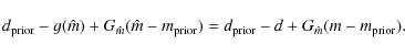
The inversion process consists in imposing that the data are linked to
the model through a theoretical mapping g: d = g(m). This is achieved by considering, as posterior information on the model, the conditional probability law for m given that the a priori random vector d - g(m) is null. In the present case of extinction, m is the opacity (or the log opacity) function over the space, and g
is given by Eq. (8). When both data and model are assumed to be
Gaussian random vectors, with the center and covariance operator
respectively denoted by
![]() ,
Cd, and
,
Cd, and
![]() ,
Cm, and when g is weakly non-linear, Tarantola & Valette (1982b) showed that the posterior measure for m can be well approximated by the Gaussian measure, the
center
,
Cm, and when g is weakly non-linear, Tarantola & Valette (1982b) showed that the posterior measure for m can be well approximated by the Gaussian measure, the
center ![]() of which makes minimum E(m)
of which makes minimum E(m)
|
(12) |
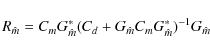
and the covariance operator of which is expressed as
| C = (Cm-1 + Gm*Cd-1Gm)-1, | (13) |
where Gm* denotes the adjoint - with respect to the usual scalar product of the model space and the data space - of the derivative Gm of g at model m. The model
| |
= | ||
| (14) |
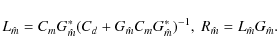
which can be solved iteratively (Tarantola & Valette 1982b) following a fixed point algorithm
| |
= | Cm Gk*( Cd + Gk Cm Gk*)-1 | |
| (15) |
where Gk denotes the derivative of g at model mk. It is important to note that even though the model (i.e. the log-opacity
|
(16) |
where
|
(17) |
where n is the number of data, and where the n-vector
|
(18) |
with
|
(19) |
3.2 Resolving power and averaging index
The concept of the resolving kernel, introduced by Backus & Gilbert (1970), is an effective tool to appreciate the efficiency of inversion. Taking that d = g(p) into account, a first order expansion of g around
![]() yields
yields
|
(20) |
Substituting this expression into Eq. (14) gives
|
(21) |
where
|
(22) |
and
|
(23) |
Expression (21) shows that correct to first order the model
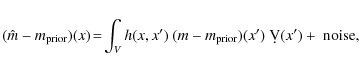
|
(24) |
where h(x,x') is the kernel of the resolution operator, which is called the resolving, or the averaging kernel. Clearly, the value of
Here we will focus on another important and useful concept, closely related to the averaging kernel.
Let (
![]() )
be the mean value of the true model within the width of the kernel around x. Equation (24) reads
)
be the mean value of the true model within the width of the kernel around x. Equation (24) reads
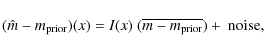
|
(25) |
where
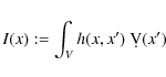
|
(26) |
is called the averaging index. In those areas where the data provide poor information, I(x) takes very low values, and hence the resulting model remains close to the prior one, independantly of the value of the true model in the neighborhood. In contrast, where the index is close to one, the resulting model corresponds to the mean value of the true model within the width of the averaging kernel. Thus, displaying the area where the index is low is a way to indicate the limit of the zone where the inference becomes poor.
3.3 Prior information on the opacity distribution
In this method the model parameters may include finite dimensional
vectors as well as functions. For finite dimensional model spaces,
Cm is
simply a matrix. In the case where we do not have any prior information
on parameters, the parameters must be a priori decorrelated
with large variances.
For functions we must define the correlation kernel
![]() of the covariance operator (16).
Simple kernels are Gaussian kernels
of the covariance operator (16).
Simple kernels are Gaussian kernels
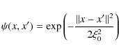
|
(27) |
or an exponential kernel
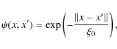
|
(28) |
where
In this study, we first used a Gaussian kernel that yielded a poor
data fit. Because the interstellar medium clearly shows different
characteristic lengths, we found it more judicious to
use multiscale kernels (Serban & Jacobsen 2001).
Actually, the introduction of two scales, the first one
characterizing the diffuse matter and the second one the compact clouds
or group of clouds, was sufficient to obtain a good adjustment of data
in a second step. The covariance kernel which we used is
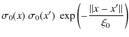
The characteristic lengths
3.4 Data adjustment
The extinction data we used are not complete in the sense that the more extinguished stars are not observed because of magnitude selection. In the core of dense clouds, extinction reaches 10 mag (Cambresy 1997) with typical cloud sizes lower than a few pc. Thus, we underestimated the opacity in the darkest regions of the sky and the star sample used in this study allows us to detect only diffuse clouds. Moreover, the real density fluctuations occur at different scales and the smoothing length allows us to detect only typical dust cloud sizes larger than 5 pc, which corresponds to the smallest correlation length used in Eq. (29). Spatial fluctuations smaller than this smoothing length are not detectable.
Some extinction data are not compatible with our model (Fig. 2), more particularly stars with large observed extinction. The colors of these stars are probably affected by structures smaller than the correlation length and cannot be taken into consideration in our model.
For this reason, Fig. 2 shows asymetric behavior: some large observed extinctions are not correctly adjusted by our model and are underestimated. Another possibility is the presence of outliers because peculiar calibration stars could not be detected during selection step.
4 Results
The result of the inversion procedure is a 1013 data cube, corresponding to a 500 ![]() 500
500 ![]() 500 pc3 cube in physical space, each individual 5
500 pc3 cube in physical space, each individual 5 ![]() 5
5 ![]() 5 pc3
pixel being attributed a volume opacity. In this section we
present the main characteristics of this opacity distribution, along
with the results of a similar inversion of 1670 interstellar
neutral sodium (NaI) column densities measured towards stars within
300 parsecs. The sodium data are those presented in Welsh
et al. (2010).
At variance with the inversion shown in Welsh et al., which
was performed for a unique kernel of 20 pc correlation length, the
present sodium inversion was done based on the same data but for
exactly the same inversion parameters as for the opacities, i.e. two
kernels with correlation lengths of 5 pc and 15 pc
respectively. One may expect some small differences from the Welsh
et al. maps, especially at the smallest scale, because the present
inversion allows for smaller clouds. The choice of identical kernels is
motivated by the need to eliminate one of the sources of potential
differences between sodium and dust opacity.
5 pc3
pixel being attributed a volume opacity. In this section we
present the main characteristics of this opacity distribution, along
with the results of a similar inversion of 1670 interstellar
neutral sodium (NaI) column densities measured towards stars within
300 parsecs. The sodium data are those presented in Welsh
et al. (2010).
At variance with the inversion shown in Welsh et al., which
was performed for a unique kernel of 20 pc correlation length, the
present sodium inversion was done based on the same data but for
exactly the same inversion parameters as for the opacities, i.e. two
kernels with correlation lengths of 5 pc and 15 pc
respectively. One may expect some small differences from the Welsh
et al. maps, especially at the smallest scale, because the present
inversion allows for smaller clouds. The choice of identical kernels is
motivated by the need to eliminate one of the sources of potential
differences between sodium and dust opacity.
![\begin{figure}
\par\includegraphics[width=8.5cm,clip]{13962fg2.eps}
\end{figure}](/articles/aa/full_html/2010/10/aa13962-09/img83.png)
|
Figure 2: Fit between modeled data and observed one. |
| Open with DEXTER | |
This parallel analysis has two main reasons. First, both neutral
sodium and opacity probe dense interstellar clouds, and it is
interesting to compare the distributions from the point of view of the
ISM itself. The second reason, more important at this stage of our
inversion studies, is technical. It is very informative to
compare two inversions based on two completely independent data sets,
because it provides some tests of the inversion, especially about the
choice of the kernels in relation with the target distribution and its
statistical significance. As we discussed earlier, the set of
target stars for the opacity study is characterized by a
non-homogeneous distribution, with some regions particularly well
covered, like the Southern hemisphere region at
![]() and
and
![]() .
Also, the density of stars decreases strongly beyond a distance
varying between 100 and 200 pc depending on the directions,
due to selection effects linked to very strong extinction. The set of
sodium target stars on the other hand is more regularly distributed
with distance, but is a factor of four smaller. It is interesting
to see the effect of such different grids on the large scale
distribution of the inverted quantity.
.
Also, the density of stars decreases strongly beyond a distance
varying between 100 and 200 pc depending on the directions,
due to selection effects linked to very strong extinction. The set of
sodium target stars on the other hand is more regularly distributed
with distance, but is a factor of four smaller. It is interesting
to see the effect of such different grids on the large scale
distribution of the inverted quantity.
4.1 Integrated opacities
4.1.1 Comparison with the Schlegel et al. full-sky dust maps
An interesting comparison can be made with the reddening maps of Schlegel et al. (1998). These two maps (for the Northern and the Southern galactic hemispheres) give the total reddening E(B-V) deduced from dust emission measurements and a temperature correction. Using our extinction cloud model, we are able to estimate the total expected extinction at high galactic latitude integrating Eq. (8) from 0 to infinity (in practice, the integration is stopped at 250 pc). In order to directly compare the results of our model with those of Schlegel et al., we used the same grid representation and interpolated the integrated extinction on a similar sampling.
![\begin{figure}
\par\includegraphics[width=8.5cm,clip]{13962fg3.eps}
\end{figure}](/articles/aa/full_html/2010/10/aa13962-09/img86.png)
|
Figure 3: Comparison between the Schlegel et al. extinction and extinction obtained in this study: north galactic pole in Lambert projection. |
| Open with DEXTER | |
![\begin{figure}
\par\includegraphics[width=8.5cm,clip]{13962fg4.eps}
\end{figure}](/articles/aa/full_html/2010/10/aa13962-09/img87.png)
|
Figure 4: Same as Fig. 3 for the south galactic pole. |
| Open with DEXTER | |
![\begin{figure}
\par\includegraphics[width=8.5cm,clip]{13962fg5.eps}
\end{figure}](/articles/aa/full_html/2010/10/aa13962-09/img88.png)
|
Figure 5: Sodium column density versus E(b-y) for common LOS. |
| Open with DEXTER | |
Figures 3 and 4 show the comparisons separately for the Northern and Southern galactic hemisphere. This clearly shows that the extinction results are compatible: the extinction structures recovered from stars are underestimated because that cloud cores are not tracked by our sample.
![\begin{figure}
\par\includegraphics[width=9cm,height=10cm]{13962fg6.eps}
\end{figure}](/articles/aa/full_html/2010/10/aa13962-09/img89.png)
|
Figure 6: Integrated opacity (resp. NaI column density) along 250 parsec long lines-of-sight based on the inverted cubes, here represented in Aitoff coordinates and linear scale. An opacity iso-contour (white line) is drawn on the sodium map for easier comparison. |
| Open with DEXTER | |
4.1.2 Comparison with integrated NaI columns
To get a first global comparison of the two inversions, we
back-integrated the cube values (the volume opacities and NaI
densities) from the center to the surface of the cubes. More
specifically, starting with the inverted cubes we computed for a
regular grid of directions and for the complete sky the total opacity
and the total NaI column integrated from the Sun up to a distance
of 250 pc. The results are displayed in Fig. 6 for a grid of directions evenly spaced by 2.5 ![]() .
.
A first look at those figures immediately reveals the local galactic disk ``warp'', clearly visible here in both the dust and gas distributions, with a general trend of concentration above the plane towards galactic longitudes 325 and 75 degrees, and below the plane elsewhere. This corresponds to the well-known Gould belt distribution of nearby O-B stars and gas. This clearly reconstructed ``warp'' in the two maps is a very encouraging result, because the ``a priori'' solutions in both cases are plane-parallel and symmetric with respect to the plane. The similarities between the two integrated quantities are also obvious when considering the large scales. This demonstrates that the stellar grids are dense enough to reveal the main concentrations of dust and gas. A closer inspection reveals some differences at the smaller angular scales, especially in the very dense regions. These differences will be more clearly visible in the 2D cuts through the cubes presented below, and may correspond to (i) inaccuracies of the inversion due to a too coarse stellar grid; (ii) actual differences between gas and dust; (iii) inaccurate data. The detailed study of all these discrepancies is a very time-consuming task, which is progressing along with the inversion of increasing amounts of targets.
A clearly revealed feature is the marked difference between the integrated opacity at the North and South poles. This is to relate to the North-South asymmetry already found by Schlegel et al. (1998) in their reconstructed dust extinction maps based on COBE/DIRBE and IRAS data. That there is significant dust and a high dust/gas ratio in the North has also been inferred from extinction and HI data in several works (Knude & Høg 1999).
![\begin{figure}
\par\includegraphics[width=14cm,height=7cm]{13962fg7.eps}
\vspace*{3mm}
\end{figure}](/articles/aa/full_html/2010/10/aa13962-09/img91.png)
|
Figure 7: Volume opacity ( left) and NaI volume density ( right) within the meridian plane. Added are several iso-contours as well as the locations (triangles) of the target stars close to the plane (see text). The marker color represents the integrated opacity (resp. column) towards the star. Small dots are plotted in areas where there are no constraints on the inversion, and the volume opacity (resp. density) is equal to the a priori value. |
| Open with DEXTER | |
Interestingly, the North-South asymmetry is not obviously present in the sodium columns, and the comparison between the two maps suggests that the dust/gas ratio is different in the two polar areas within 250 parsecs. This difference, which will probably have some consequences in the context of dust emission models, certainly deserves further studies.
4.2 Cuts in the 3D opacity and density cubes, identification of structures
In this section we show the volume opacity and NaI density within several planes, i.e. different cuts in the 3D inverted cubes. For each map the continuous value of the volume opacity (resp. density) is shown with some iso- volume opacity (iso-volume density) contours drawn to help visualize the dense areas and the voids. Also shown are the stars which are close to the plane and have contributed to the adjustment. The criterion for keeping the stars is identical to that presented in Sfeir et al. (1999). The color scale for the stars corresponds to the measured integrated opacity (resp. column density) between the Sun and the star. This allows us to figure out how many stars have constrained the inversion and which stars have most influenced the local opacity (density).
Also shown in the maps are some markers of the reliability of the inversion process, which is directly linked to the number of targets and their spatial distributions: areas with an averaging index lower than 0.5 are marked by black dots. In almost all maps, the inversion is well-constrained within 100-150 parsecs, while beyond these distances there are large differences according to the longitude or latitude. The most constrained plane for neutral sodium is the Gould belt plane, because there are numerous nearby early-type stars along the belt, which are ideal targets. High-latitude areas are not well-sampled, with the exception of the poles themselves or well-known ``windows'' of low columns.
4.2.1 Vertical planes
Figures 7 to 10 display the inverted volume opacity and Na density in four vertical planes containing the Sun at 45 ![]() from
each other, starting with the meridian plane, i.e. the vertical
plane which contains the galactic center and anti-center directions.
These vertical planes are the most appropriate cuts in the
3D cubes for revealing the limits of the inversion process linked
to the data sets, because the space density of the targets decreases
strongly with the distance to the plane. Indeed, the influence of
the ``a priori distribution'' can be easily discerned in those
maps in all unconstrained areas in the form of a smooth decrease of the
opacity (density) as a function of the distance to the plane and
horizontal iso-densities. This is a visible criterion of a lack of
constraints.
from
each other, starting with the meridian plane, i.e. the vertical
plane which contains the galactic center and anti-center directions.
These vertical planes are the most appropriate cuts in the
3D cubes for revealing the limits of the inversion process linked
to the data sets, because the space density of the targets decreases
strongly with the distance to the plane. Indeed, the influence of
the ``a priori distribution'' can be easily discerned in those
maps in all unconstrained areas in the form of a smooth decrease of the
opacity (density) as a function of the distance to the plane and
horizontal iso-densities. This is a visible criterion of a lack of
constraints.
On the other hand, the juxtaposition of the same maps drawn from opacity and neutral sodium also clearly reveals the limitations of the 3D reconstruction. In some locations there are several differences between the centroids of the dense areas, or the absence of a feature in one of the two maps. Those shortcomings are related to the target scarcity in some areas or may also be related to parallax uncertainties.
Despite these limitations, the Local Cavity is clearly defined in each
of the vertical planes, and as noted in our previous works,
is significantly inclined with respect to the plane. The global
inclination reaches maxima in the 0-180 ![]() meridian plane and in the 315-135
meridian plane and in the 315-135 ![]() vertical plane, and the maps suggest a complicated structure with a
number of low-density chimneys linking the cavity to the halo.
vertical plane, and the maps suggest a complicated structure with a
number of low-density chimneys linking the cavity to the halo.
![\begin{figure}
\par\includegraphics[width=14cm,height=7cm]{13962fg8.eps}
\end{figure}](/articles/aa/full_html/2010/10/aa13962-09/img92.png)
|
Figure 8:
Same as Fig. 7 within a vertical plane at 45 |
| Open with DEXTER | |
![\begin{figure}
\par\includegraphics[width=14cm,height=7cm]{13962fg9.eps}
\end{figure}](/articles/aa/full_html/2010/10/aa13962-09/img93.png)
|
Figure 9: Same as Fig. 7 within the rotation plane. |
| Open with DEXTER | |
![\begin{figure}
\par\includegraphics[width=14cm,height=7cm]{13962fg10.eps}
\end{figure}](/articles/aa/full_html/2010/10/aa13962-09/img94.png)
|
Figure 10:
Same as Fig. 7 within a vertical plane at 45 |
| Open with DEXTER | |
Some nearby cavities are revealed by those vertical maps, almost in all
cases in both extinction and gas maps when there are constraints in
those areas, but frequently the dust or gas distributions around the
cavities differ slightly or more significantly, due to the target
limitations.
Work is in progress to identify these cavities in radio and X-ray maps
and will be the subject of a forthcoming paper (Raimond et al.
2010). We identified a few structures in the meridian plane in
Fig. 7. The distances to Taurus and ![]() Oph clouds will be discussed in the next section. The nearby Corona Australis concentration of clouds at -20
Oph clouds will be discussed in the next section. The nearby Corona Australis concentration of clouds at -20 ![]() is present but there are some substantial differences in the structure
derived from extinction and the sodium inversion. These differences may
be due to the scarcity of target stars in this area and the small size
of the CrA molecular region. The distance to the densest area in
this direction is 135 pc from extinction, and about 165 pc on
the sodium map. The former distance corresponds to previous estimates
and the latter to the estimate by Knude & Hög (1998). More data are required in this area.
is present but there are some substantial differences in the structure
derived from extinction and the sodium inversion. These differences may
be due to the scarcity of target stars in this area and the small size
of the CrA molecular region. The distance to the densest area in
this direction is 135 pc from extinction, and about 165 pc on
the sodium map. The former distance corresponds to previous estimates
and the latter to the estimate by Knude & Hög (1998). More data are required in this area.
![\begin{figure}
\par\includegraphics[width=14cm,clip]{13962fg11.eps}
\vspace*{6.5mm}
\end{figure}](/articles/aa/full_html/2010/10/aa13962-09/img96.png)
|
Figure 11: Volume opacity within the Gould Belt plane (orientation taken from Perrot & Grenier 2003). |
| Open with DEXTER | |
4.2.2 The Gould belt/Lindblad ring plane
![\begin{figure}
\par\includegraphics[width=14cm,clip]{13962fg12.eps}
\vspace*{2.5mm}
\end{figure}](/articles/aa/full_html/2010/10/aa13962-09/img97.png)
|
Figure 12: Same as Fig. 11 for the neutral sodium volume density. |
| Open with DEXTER | |
In opposition to the vertical planes, the galactic plane and the Gould belt/Lindblad ring (GB) plane (see Pöppel (1997) for a recent review on this structure) are among the most favorable regions for the inversion from the point of view of target distribution. For the extinction stellar data set, the galactic plane is the most appropriate, but the Gould belt plane, being only slightly inclined, also contains a high density of targets. For the sodium absorption data set it is the most appropriate, because it contains a large amount of bright, early-type stars that constitute ideal targets. On the other hand, the GB plane is highly structured because it contains most of the dark clouds, star-forming regions, and HII regions. Although this complexity makes the inversion more difficult, it is interesting to attempt a mapping within this plane. We have thus chosen to display the inversion results within this particular plane, and the corresponding cuts in the two inverted cubes are displayed in Figs. 11 and 12.
The Gould belt/Lindblad ring structure has been the subjects of
extensive studies, and we have chosen here for the definition of the
plane the coordinates calculated by Perrot & Grenier (2003), based on the distribution and kinematics of OB associations and HI and H2 clouds.
It is generally admitted that the belt, whose origin is still
controversial, is about 600 pc wide and that the Sun lies
within about 150 pc from its closest part, the Scorpius-Ophuchus
complex of OB associations and dense clouds. The opacity and gas
maps both reveal this complex area, and locate the East and West
Ophiuchus clouds and the Lupus clouds from 100
to 165 pc, in agreement with the recent work of Snow
et al. (2008) from absorption data (122 ![]() 8 pc for the densest part of
8 pc for the densest part of ![]() Oph and 133-150 pc for its western part), and Lombardi et al. (2008) from reddening data (119
Oph and 133-150 pc for its western part), and Lombardi et al. (2008) from reddening data (119 ![]() 6 pc for the densest part of
6 pc for the densest part of ![]() Oph and 155
Oph and 155 ![]() 8 pc for Lupus). The advantage of the present map compared to
these two specific studies is that it provides a global view of this
entire region as well as the continuity between these regions.
Similarly the map reveals the structure of the Coalsack
(its southern part only is within this plane) and Chameleon dark
clouds at distances similar to the previous results of Knude & Høg (1998).
These authors found between 100 and 150 pc for South
Coalsack, which corresponds well to the elongated dense area in our
map, and two separate dense regions for Chameleon, the densest at about
150 pc and the second much closer, starting at about 80 pc.
This again corresponds well to the double structure we find in this
direction. Opposite to this dense region is the Taurus dark cloud
complex at about the same distance (150 pc), in agreement
with previous work on the young objects and molecular clouds in this
area (Bertout et al. 1999).
The star distribution allows the detection beyond Taurus of the closest
part of the giant Orion-Eridanus superbubble, along with some nearby
condensations at its periphery. The Local Cavity is opening into
another giant cavity, the GS238+00+09 superbubble (Heiles 1998), adjacent to Orion-Eridanus. Interestingly, the Local Cavity has two extensions at l=85
8 pc for Lupus). The advantage of the present map compared to
these two specific studies is that it provides a global view of this
entire region as well as the continuity between these regions.
Similarly the map reveals the structure of the Coalsack
(its southern part only is within this plane) and Chameleon dark
clouds at distances similar to the previous results of Knude & Høg (1998).
These authors found between 100 and 150 pc for South
Coalsack, which corresponds well to the elongated dense area in our
map, and two separate dense regions for Chameleon, the densest at about
150 pc and the second much closer, starting at about 80 pc.
This again corresponds well to the double structure we find in this
direction. Opposite to this dense region is the Taurus dark cloud
complex at about the same distance (150 pc), in agreement
with previous work on the young objects and molecular clouds in this
area (Bertout et al. 1999).
The star distribution allows the detection beyond Taurus of the closest
part of the giant Orion-Eridanus superbubble, along with some nearby
condensations at its periphery. The Local Cavity is opening into
another giant cavity, the GS238+00+09 superbubble (Heiles 1998), adjacent to Orion-Eridanus. Interestingly, the Local Cavity has two extensions at l=85 ![]() and
l=240-250
and
l=240-250 ![]() in this plane, which are nearly perpendicular to the axis defined by
the densest regions of Taurus and Sco-Oph. The longest extension
coïncides with the well-know Canis Major extended void.
in this plane, which are nearly perpendicular to the axis defined by
the densest regions of Taurus and Sco-Oph. The longest extension
coïncides with the well-know Canis Major extended void.
Again the comparison between the two distributions agree very well
about the global structure, which shows that the two data sets are good
enough for this large-scale determination. On the other hand, there are
differences in the detailed structure. Work is in progress to identify
the molecular complexes detected in radio data, and preliminary results
confirm that while some of the smallest isolated clouds are missed due
to insufficient sky coverage, the main concentrations are retrieved.
Further investigations are necessary in those cases, both the opacity
and sodium star distributions are generally not sufficient to answer
the remaining questions. The most important difference is at l=235 ![]() ,
at a distance of about 200 pc. Here the dense
concentration detected in sodium does not seem to have a similarly
strong counterpart in opacity. It is the reverse in the opposite
direction, at about 120 pc. Is this due to a strongly
variable dust-to-gas ratio, or to an artefact?
,
at a distance of about 200 pc. Here the dense
concentration detected in sodium does not seem to have a similarly
strong counterpart in opacity. It is the reverse in the opposite
direction, at about 120 pc. Is this due to a strongly
variable dust-to-gas ratio, or to an artefact?
From those maps and the distribution of the quality index, it is clear that there is a lack of targets beyond the densest concentrations. It is not clear e.g. where the dust and gas densities drop beyond the Sco-Oph and Lupus clouds, or beyond Taurus. This is an important aspect, because the precise localization of the nearby cavities, which are potential X-ray emitters, would be a valuable advance.
5 Conclusions
We built a carefully and conservatively selected list of opacity measurements based on Strömgren photometry, restricted to nearby stars possessing a Hipparcos parallax and located within 300 pc. We inverted this opacity database (6400 targets) together with the interstellar sodium absorption database (1650 targets) presented in Welsh et al. (2010) by means of an inversion tool specifically adjusted to those data. We compared the resulting 3D dust and gas distributions in different ways, including maps of integrated opacity and density as well as planar cuts within the 3D cubes.
The main conclusions of those inversions are:
- Integrals over 250 parsecs of the reconstructed opacities and sodium densities show very similar patterns over the sky and reveal in a similar fashion the local warp of the plane, a warp link to the Gould belt-Lindblad ring global structure.
- The comparison with the integrated opacities from Schlegel et al. (1998) shows that the present results are compatible with those obtained from dust emission maps.
- The extinction maps suggest a higher dust content at high galactic latitude in the Northern hemisphere compared to the South, while the gas maps do not. There is thus evidence for a higher dust-to-gas ratio in the North, in agreement with previous evidences (Knude & Høg 1999).
- Both tracers clearly reveal the Local Cavity and its contours are similar in both pictures, despite the totally independent and indeed very different data sets.
- In general the large scale structures agree well everywhere there are constraints from the data.
- At smaller scale there are some differences, which may be real, but in most cases are likely due to the limited target coverage. This is clearly seen in the maps, especially far from the plane in the vertical cuts. Work is in progress on those discrepancies.
We sincerely thank our referee J. Knude for the careful reading of our manuscript and constructive comments as well as for his prompt review. This research has extensively used the Simbad database and on-line facility, operated by the CDS (Strasbourg, France). A large faction of the absorption data are based on observations collected at the European Southern Observatory, La Silla, Chile.
References
- Backus, G., & Gilbert, F. 1970, Phil. Trans. R. Soc. London, 266, 123 [Google Scholar]
- Bertout, C., Robichon, N., & Arenou, F. 1999, A&A, 352, 574 [NASA ADS] [Google Scholar]
- Blitz, L., Fich, M., & Stark, A. A. 1982, ApJSS, 49,183 [CrossRef] [Google Scholar]
- Bradley, W. C., & Dale, A. O. 1996, An introduction to modern astrophysics (Addison-Wesley Publishing Company, Inc.) [Google Scholar]
- Cambresy, L., Epchtein, N., Copet, E., et al. 1997, A&A, 324, L5 [NASA ADS] [Google Scholar]
- Chen, B., Vergely, J.-L., Valette, B., & Carraro, G. 1998, A&A, 336, 137 [NASA ADS] [Google Scholar]
- Corradi, W. J. B., Franco, G. A. P., & Knude, J. 2004, MNRAS, 347, 1065 [NASA ADS] [CrossRef] [Google Scholar]
- Cox, D. P. 1998, The Local Bubble and Beyond, IAU Colloq., 506, 121 [Google Scholar]
- Cox, D. P. 2005, ARA&A, 43, 337 [NASA ADS] [CrossRef] [EDP Sciences] [MathSciNet] [Google Scholar]
- Cox, D. P., & Reynolds, R. J. 1987, ARA&A, 25, 303 [NASA ADS] [CrossRef] [Google Scholar]
- Craig, I. J. D., & Brown, J. C. 1986, Inverse Problems in Astronomy (Bristol and Boston: Adam Hilger Ltd) [Google Scholar]
- Cravens, T. E. 2000, ApJ, 532, L153 [NASA ADS] [CrossRef] [PubMed] [Google Scholar]
- Crawford, D. L. 1975, AJ, 80, 955 [NASA ADS] [CrossRef] [Google Scholar]
- Crawford, D. L. 1978, AJ, 83, 48 [NASA ADS] [CrossRef] [Google Scholar]
- Crawford, D. L. 1979, AJ, 84, 1858 [NASA ADS] [CrossRef] [Google Scholar]
- de Avillez, M., & Breitschwerdt, D. 2004, Ap&SS, 289, 479 [NASA ADS] [CrossRef] [Google Scholar]
- Draine, B. T. 2003, ARA&A, 41, 241 [NASA ADS] [CrossRef] [Google Scholar]
- Draine, B. T. 2004, Origin and Evolution of the Elements, 317 [Google Scholar]
- Ducati, J. R. 1986, Ap&SS, 126, 269 [NASA ADS] [CrossRef] [Google Scholar]
- Fitzgerald, M. P. 1968, AJ, 73, 983 [NASA ADS] [CrossRef] [Google Scholar]
- Frisch, P. C., & York, D. G. 1983, ApJ, 271, L59 [NASA ADS] [CrossRef] [Google Scholar]
- Génova, R., & Beckman, J. E. 2003, ApJS, 145, 355 [NASA ADS] [CrossRef] [Google Scholar]
- Guarinos, J. 1991, Ph.D. Thesis, Observatoire de Strasbourg, France [Google Scholar]
- Guillout, P., Sterzik, M. F., Schmitt, J. H. M. M., Motch, C., & Neuhaeuser, R. 1998, A&A, 337, 113 [NASA ADS] [Google Scholar]
- Hauck, B., & Mermilliod, M. 1990, A&AS, 86, 107 [Google Scholar]
- Hauck, B., & Mermilliod, M. 1998, A&AS, 129, 431 [NASA ADS] [CrossRef] [EDP Sciences] [Google Scholar]
- Heiles, C. 1998, ApJ, 498, 689 [NASA ADS] [CrossRef] [Google Scholar]
- Hilditch, R. W., Hill, G., & Barnes, J. V. 1983, MNRAS, 204, 241 [NASA ADS] [CrossRef] [Google Scholar]
- Jenkins, E. B. 2009, Space Sci. Rev., 143, 205 [NASA ADS] [CrossRef] [Google Scholar]
- Knauth, D. C., Howk, J. C., Sembach, K. R., Lauroesch, J. T., & Meyer, D. M. 2003, ApJ, 592, 964 [NASA ADS] [CrossRef] [Google Scholar]
- Knude, J., & Høg, E. 1998, A&A, 338, 897 [NASA ADS] [Google Scholar]
- Knude, J., & Høg, E. 1999, A&A, 341, 451 [NASA ADS] [Google Scholar]
- Koutroumpa, D., Lallement, R., Raymond, J., & Kharchenko, V. 2009, ApJ, 696, 1517 [NASA ADS] [CrossRef] [Google Scholar]
- Kraütter, J. 1980, A&A, 89, 74 [NASA ADS] [Google Scholar]
- Lallement, R. 2009, Space Sci. Rev., 143, 427 [NASA ADS] [CrossRef] [Google Scholar]
- Lallement, R., Ferlet, R., Lagrange, A. M., Lemoine, M., & Vidal-Madjar, A. 1995, A&A, 304, 461 [NASA ADS] [Google Scholar]
- Lallement, R., Welsh, B. Y., Vergely, J. L., et al. 2003, A&A, 411, 447 [EDP Sciences] [Google Scholar]
- Lallement, R., Hébrard, G., & Welsh, B. Y. 2008, A&A, 481, 381 [NASA ADS] [CrossRef] [EDP Sciences] [Google Scholar]
- Lombardi, M., Lada, C. J., & Alves, J. 2008, A&A, 480, 785 [NASA ADS] [CrossRef] [EDP Sciences] [Google Scholar]
- Lucke, P. B. 1978, A&A, 64, 367 [NASA ADS] [Google Scholar]
- Lyngå, G. 1987, Catalogue of Open Cluster Data, 5th edition [Google Scholar]
- Lynds, B. 1974, ApJSS, 28, 391 [NASA ADS] [CrossRef] [Google Scholar]
- Linsky, J. L., Draine, B. T., Moos, H. W., et al. 2006, ApJ, 647, 1106 [NASA ADS] [CrossRef] [Google Scholar]
- Meyer, D., Lauroesch, J., Heiles, C., et al. 2006, ApJ, 650, L67 [NASA ADS] [CrossRef] [Google Scholar]
- Neckel, T., & Klare, G. 1980, A&AS, 42, 251 [Google Scholar]
- Perrot, C. A., & Grenier, I. A. 2003, A&A, 404, 519 [NASA ADS] [CrossRef] [EDP Sciences] [Google Scholar]
- Perryman, M. A. C., Lindegren, L., Kovalevsky, J., et al. 1997, A&A, 323, L49 [NASA ADS] [Google Scholar]
- Philip, A. D., & Egret, D. 1980, A&AS, 40, 199 [Google Scholar]
- Poppel, W. 1997, Fundamentals of Cosmic Physics, 18, 1 [Google Scholar]
- Redfield, S., & Linsky, J. L. 2008, ApJ, 673, 283 [NASA ADS] [CrossRef] [Google Scholar]
- Reis, W., & Corradi, W. J. B. 2008, A&A, 486, 471 [NASA ADS] [CrossRef] [EDP Sciences] [Google Scholar]
- Rodgers, C. D. 2008, Inverse methods for atmospheric sounding, Theory and Practice (World Scientific) [Google Scholar]
- Savage, B. D., & Lehner, N. 2006, ApJS, 162, 134 [NASA ADS] [CrossRef] [Google Scholar]
- Serban, D. Z., & Jacobsen, B. H. 2001, Geophys. J. Int., 147, 29 [NASA ADS] [CrossRef] [Google Scholar]
- Sfeir, D., Lallement, R., Crifo, F., & Welsh, B. Y. 1999, A&A, 346, 785 [NASA ADS] [Google Scholar]
- Shlegel, D. J., Finkbeiner, D. P., & Davis, M. 1998, ApJ, 500, 525 [NASA ADS] [CrossRef] [Google Scholar]
- Slavin, J. D. 1989, ApJ, 346, 718 [NASA ADS] [CrossRef] [Google Scholar]
- Snowden, S., Freyberg, M., Kuntz, K., & Sanders, W. 2000, ApJS, 128, 171 [NASA ADS] [CrossRef] [Google Scholar]
- Snow, T. P., Destree, J. D., & Welty, D. E. 2008, ApJ, 679, 512 [NASA ADS] [CrossRef] [Google Scholar]
- Tarantola, A., & Valette, B. 1982a, J. Geophys., 50, 159 [Google Scholar]
- Tarantola, A., & Valette, B. 1982b, Rev. Geo. Space Phys., 20, 219 [Google Scholar]
- Twomey, S. 1977, Inversion Methods in Atmospheric Remote Sounding, 4, 41 [NASA ADS] [Google Scholar]
- van Leeuwen, F. 2007, A&A, 474, 653 [NASA ADS] [CrossRef] [EDP Sciences] [Google Scholar]
- Vergely, J.-L., Egret, D., Freire Ferrero, R., & Köppen, J. 1997, ESA SP, 402, 603 [Google Scholar]
- Vergely, J.-L., Ferrero, R. F., Egret, D., & Koeppen, J. 1998, A&A, 340, 543 [NASA ADS] [Google Scholar]
- Vergely, J.-L., Freire Ferrero, R., Siebert, A., & Valette, B. 2001, A&A, 366, 1016 [NASA ADS] [CrossRef] [EDP Sciences] [Google Scholar]
- Welsh, B. Y., & Lallement, R. 2005, A&A, 436, 615 [NASA ADS] [CrossRef] [EDP Sciences] [Google Scholar]
- Welsh, B. Y., Lallement, R., Vergely, J. L., & Raimond, S. 2010, A&A, 510, A54 [NASA ADS] [CrossRef] [EDP Sciences] [Google Scholar]
Footnotes
- ... gas
- Partly based on observations collected at the European Southern Observatory, La Silla, Chile.
All Tables
Table 1: Distribution of the sample stars into four Strömgren groups (before parallax selection).
Table 2: Estimation of errors and biases on extinction according to the group of calibration for stars in the 70 pc sphere.
All Figures
|
|
Figure 1: Histogram extinction for stars in the 70 pc sphere. |
| Open with DEXTER | |
| In the text | |
|
|
Figure 2: Fit between modeled data and observed one. |
| Open with DEXTER | |
| In the text | |
|
|
Figure 3: Comparison between the Schlegel et al. extinction and extinction obtained in this study: north galactic pole in Lambert projection. |
| Open with DEXTER | |
| In the text | |
|
|
Figure 4: Same as Fig. 3 for the south galactic pole. |
| Open with DEXTER | |
| In the text | |
|
|
Figure 5: Sodium column density versus E(b-y) for common LOS. |
| Open with DEXTER | |
| In the text | |
|
|
Figure 6: Integrated opacity (resp. NaI column density) along 250 parsec long lines-of-sight based on the inverted cubes, here represented in Aitoff coordinates and linear scale. An opacity iso-contour (white line) is drawn on the sodium map for easier comparison. |
| Open with DEXTER | |
| In the text | |
|
|
Figure 7: Volume opacity ( left) and NaI volume density ( right) within the meridian plane. Added are several iso-contours as well as the locations (triangles) of the target stars close to the plane (see text). The marker color represents the integrated opacity (resp. column) towards the star. Small dots are plotted in areas where there are no constraints on the inversion, and the volume opacity (resp. density) is equal to the a priori value. |
| Open with DEXTER | |
| In the text | |
|
|
Figure 8:
Same as Fig. 7 within a vertical plane at 45 |
| Open with DEXTER | |
| In the text | |
|
|
Figure 9: Same as Fig. 7 within the rotation plane. |
| Open with DEXTER | |
| In the text | |
|
|
Figure 10:
Same as Fig. 7 within a vertical plane at 45 |
| Open with DEXTER | |
| In the text | |
|
|
Figure 11: Volume opacity within the Gould Belt plane (orientation taken from Perrot & Grenier 2003). |
| Open with DEXTER | |
| In the text | |
|
|
Figure 12: Same as Fig. 11 for the neutral sodium volume density. |
| Open with DEXTER | |
| In the text | |
Copyright ESO 2010
Current usage metrics show cumulative count of Article Views (full-text article views including HTML views, PDF and ePub downloads, according to the available data) and Abstracts Views on Vision4Press platform.
Data correspond to usage on the plateform after 2015. The current usage metrics is available 48-96 hours after online publication and is updated daily on week days.
Initial download of the metrics may take a while.