| Issue |
A&A
Volume 518, July-August 2010
Herschel: the first science highlights
|
|
|---|---|---|
| Article Number | A22 | |
| Number of page(s) | 9 | |
| Section | Astrophysical processes | |
| DOI | https://doi.org/10.1051/0004-6361/200913722 | |
| Published online | 25 August 2010 | |
Open and closed boundaries in large-scale convective dynamos
P. J. Käpylä1,2 - M. J. Korpi1,2 - A. Brandenburg2,3
1 - Department of Physics, Gustaf Hällströmin katu 2a,
PO Box 64, 00014 University of Helsinki, Finland
2 - NORDITA, Roslagstullsbacken
23, 10691 Stockholm, Sweden
3 - Department of Astronomy, Stockholm University, 10691
Stockholm, Sweden
Received 23 November 2009 / Accepted 26 May 2010
Abstract
Context. Earlier work has suggested that large-scale dynamos
can reach and maintain equipartition field strengths on a dynamical
time scale only if magnetic helicity of the fluctuating field can be
shed from the domain through open boundaries.
Aims. Our aim is to test this scenario in convection-driven dynamos by comparing results for open and closed boundary conditions.
Methods. Three-dimensional numerical simulations of turbulent
compressible convection with shear and rotation are used to study the
effects of boundary conditions on the excitation and saturation of
large-scale dynamos. Open (vertical-field) and closed (perfect-
conductor) boundary conditions are used for the magnetic field. The
shear flow is such that the contours of shear are vertical, crossing
the outer surface, and are thus ideally suited for driving a
shear-induced magnetic helicity flux.
Results. We find that for given shear and rotation rate, the
growth rate of the magnetic field is larger if open boundary conditions
are used. The growth rate first increases for small magnetic Reynolds
number, ![]() ,
but then levels off at an approximately constant value for intermediate values of
,
but then levels off at an approximately constant value for intermediate values of ![]() .
For large enough
.
For large enough ![]() ,
a small-scale dynamo is excited and the growth rate of the field in this regime increases as
,
a small-scale dynamo is excited and the growth rate of the field in this regime increases as
![]() .
Regarding the nonlinear regime, the saturation level of the energy of the total magnetic field is independent of
.
Regarding the nonlinear regime, the saturation level of the energy of the total magnetic field is independent of ![]() when open boundaries are used. In the case of perfect-conductor
boundaries, the saturation level first increases as a function of
when open boundaries are used. In the case of perfect-conductor
boundaries, the saturation level first increases as a function of ![]() ,
but then decreases proportional to
,
but then decreases proportional to
![]() for
for
![]() ,
indicative of catastrophic quenching. These results suggest that the
shear-induced magnetic helicity flux is efficient in alleviating
catastrophic quenching when open boundaries are used. The horizontally
averaged mean field is still weakly decreasing as a function of
,
indicative of catastrophic quenching. These results suggest that the
shear-induced magnetic helicity flux is efficient in alleviating
catastrophic quenching when open boundaries are used. The horizontally
averaged mean field is still weakly decreasing as a function of ![]() even for open boundaries.
even for open boundaries.
Key words: magnetohydrodynamics - convection - turbulence - magnetic fields - stars: magnetic field - magnetic fields
1 Introduction
The classical view of the effect of shear in large-scale dynamos is that it promotes the generation of magnetic fields, and that it is instrumental in exciting oscillatory solutions (e.g. Parker 1955; Steenbeck & Krause 1969). While these aspects remain unchanged, a much more subtle effect of shear has been discovered in studies of the saturation mechanism of the large-scale dynamo. If the saturation of the dynamo occurs due to magnetic helicity conservation, a fully periodic or closed system experiences catastrophic quenching with the energy of the large-scale magnetic field decreasing in inverse proportion to the magnetic Reynolds number (Vainshtein & Cattaneo 1992; Cattaneo & Hughes 1996; Brandenburg 2001). A way to avoid catastrophic quenching is to allow magnetic helicity fluxes to escape from the system through open boundaries, thus allowing the large-scale fields to saturate at equipartition strength in a dynamical time scale (Blackman & Field 2000; Kleeorin et al. 2000). One of the most promising mechanisms, introduced by Vishniac & Cho (2001), operates by driving a flux of magnetic helicity along the isocontours of shear. Forced turbulence simulations with shear have confirmed that the quenching of theRecent numerical experiments with forced turbulence
(Brandenburg 2005; Yousef et al. 2008a,b; Brandenburg et al. 2008) and
convection (Käpylä et al. 2008, hereafter Paper I; Hughes
& Proctor 2009; see also Käpylä et al. 2010) with
imposed large-scale shear flows have
established the existence of a robust large-scale dynamo. The origin
of this dynamo is still under debate (shear-current versus incoherent
![]() -shear effects).
This is discussed in detail elsewhere
(e.g. Brandenburg et al. 2008; Käpylä et al. 2009b).
In forced turbulence simulations with fully periodic boundaries,
that do not allow magnetic helicity fluxes, large-scale magnetic
fields show slow saturation on a diffusive timescale (Brandenburg 2001).
Earlier results from convection also suggest that no appreciable
large-scale magnetic fields are seen if magnetic helicity fluxes are
suppressed (Paper I).
-shear effects).
This is discussed in detail elsewhere
(e.g. Brandenburg et al. 2008; Käpylä et al. 2009b).
In forced turbulence simulations with fully periodic boundaries,
that do not allow magnetic helicity fluxes, large-scale magnetic
fields show slow saturation on a diffusive timescale (Brandenburg 2001).
Earlier results from convection also suggest that no appreciable
large-scale magnetic fields are seen if magnetic helicity fluxes are
suppressed (Paper I).
In most of the simulations of Paper I the isocontours of shear were vertical
and thus intersecting the boundaries.
However, the boundary conditions (bc) imposed on the magnetic
field on the vertical borders
would either allow (open vertical-field bc) or
inhibit (closed perfect-conductor bc) a net flux
out of the domain. It was shown that when
the flux is suppressed, only weak large-scale magnetic fields occur
in the saturated state at large ![]() .
Conversely, allowing a flux produced a significant large-scale
field. Furthermore, using a similar setup as in Tobias et al. (2008), where the isocontours of shear are
horizontal, a similar effect was found. Thus it would appear that the
shear-induced flux plays a critical role in exciting a large-scale
dynamo in turbulent convection.
This has given rise to the impression that the dynamos seen
in Paper I are solely due to the magnetic helicity flux and thus inherently
nonlinear (Hughes & Proctor 2009). In the present paper we
argue that this interpretation is incorrect and that the lack of
appreciable large-scale magnetic fields
in some of our earlier cases with vanishing
helicity flux is due to the fact that the critical dynamo number for the
excitation of the dynamo is larger in that case.
We also note that, more recently, large-scale dynamos have been found in
turbulent convection without shear (Käpylä et al. 2009a),
irrespective of the presence of magnetic helicity fluxes.
.
Conversely, allowing a flux produced a significant large-scale
field. Furthermore, using a similar setup as in Tobias et al. (2008), where the isocontours of shear are
horizontal, a similar effect was found. Thus it would appear that the
shear-induced flux plays a critical role in exciting a large-scale
dynamo in turbulent convection.
This has given rise to the impression that the dynamos seen
in Paper I are solely due to the magnetic helicity flux and thus inherently
nonlinear (Hughes & Proctor 2009). In the present paper we
argue that this interpretation is incorrect and that the lack of
appreciable large-scale magnetic fields
in some of our earlier cases with vanishing
helicity flux is due to the fact that the critical dynamo number for the
excitation of the dynamo is larger in that case.
We also note that, more recently, large-scale dynamos have been found in
turbulent convection without shear (Käpylä et al. 2009a),
irrespective of the presence of magnetic helicity fluxes.
The origin of the dynamos reported in Paper I was interpreted in the context of turbulent dynamo theory in Käpylä et al. (2009b). An important feature of turbulent dynamos is that according to standard mean-field theory neither the turbulent transport coefficients nor the growth rate of the field should depend on the microscopic resistivity. The former prediction was confirmed by Käpylä et al. (2009b), but the latter has not yet been studied in detail in direct simulations. This is one of the goals of the present paper.
Another aim is to study the saturation
behaviour of the large-scale dynamo with both open and closed boundary
conditions. Firstly, in homogeneous systems, i.e. where the turbulent
transport coefficients do not vary in space,
full saturation is expected to
occur on a slow diffusive time scale with closed boundaries
whereas with open boundaries the
saturation is expected to happen on a dynamical time scale if a
helicity flux is present (Brandenburg 2001).
However, in inhomogeneous systems the situation is likely to be
more complex (e.g. Mitra et al. 2010).
Furthermore, simulations of helically forced isotropic
turbulence have shown that, in the absence of shear, the saturation
level of the magnetic field scales as
![]() for open boundaries
(Fig. 2 of Brandenburg & Subramanian 2005a).
When shear is present, the shear-induced magnetic
helicity flux should alleviate the
for open boundaries
(Fig. 2 of Brandenburg & Subramanian 2005a).
When shear is present, the shear-induced magnetic
helicity flux should alleviate the ![]() -dependence of the saturation
level. Preliminary results in Paper I indicate that this might indeed be
true, but the results are not fully conclusive because other parameters, such
as the Rayleigh number and the fluid Reynolds number changed when
-dependence of the saturation
level. Preliminary results in Paper I indicate that this might indeed be
true, but the results are not fully conclusive because other parameters, such
as the Rayleigh number and the fluid Reynolds number changed when
![]() was varied. In the present paper we perform a more detailed
study where only
was varied. In the present paper we perform a more detailed
study where only ![]() is varied.
is varied.
2 Model and methods
2.1 Setup and boundary conditions
We use the same setup as in Paper I in which a small rectangular portion of a star is modelled by a box situated at colatitudeThe values (z1, z2, z3, z4) = (-0.85, 0, 1, 1.15)d give the vertical positions of the bottom of the box, the bottom and top of the convectively unstable layer, and the top of the box, respectively. We use a heat conductivity profile such that the associated hydrostatic reference solution is piecewise polytropic with indices (m1, m2, m3)=(3, 1, 1). We apply a cooling term in the thin uppermost layer which makes this region nearly isothermal and hence stably stratified. The bottom layer is also stably stratified, and the middle layer is convectively unstable.
At the vertical boundaries we use stress-free boundary conditions for
the velocity,
| Ux,z = Uy,z = Uz = 0. | (1) |
For the magnetic field either vertical-field or perfect-conductor boundary conditions are used. Occasionally we refer to them also as open and closed, respectively. Thus, we have
the former allowing magnetic helicity flux while the latter one does not. This also motivates the usage of the names ``open'' and ``closed'' for the two boundary conditions. The y-direction is periodic and shearing-periodic conditions are used in the x-direction (e.g. Wisdom & Tremaine 1988). A constant temperature gradient is maintained at the base which leads to a steady influx of heat due to the constant heat conductivity.
The simulations were performed with the P ENCIL C ODE![]() ,
which uses sixth-order explicit finite differences in space and
third-order accurate time stepping method.
Resolutions of up to 5123 mesh points were used.
,
which uses sixth-order explicit finite differences in space and
third-order accurate time stepping method.
Resolutions of up to 5123 mesh points were used.
Table 1:
Summary of the runs with varying ![]() .
.
2.2 Units, nondimensional quantities, and parameters
Dimensionless quantities are obtained by setting
| (4) |
where g is the constant acceleration due to gravity,
| [x] | = | ||
| = | (5) |
The system is controlled by the Prandtl, Reynolds, and Rayleigh numbers,
| |
= | (6) | |
| = | (7) | ||
| = | 
|
(8) |
where
|
(9) |
with
The degree of stratification is controlled by the parameter
| (10) |
where e0 is the internal energy at z=z4. The internal energy is related to the temperature via
The strengths of rotation and shear are quantified by the Coriolis and
shear numbers
| (11) |
where
2.3 Characterization of the simulation data
Our runs can be characterized using the following quantities.
We express the rms velocity in the unit of
(gd)1/2,
which is related to the Mach number, and thus define
|
(12) |
The normalized growth rate of magnetic field is expressed as

|
(13) |
The typical wavenumber of the energy-carrying eddies and the relative kinetic helicity are given by
|
(14) |
where
|
(15) |
where
|
(16) |
and
Error bars are estimated by dividing the time series into three equally long parts and computing a mean value individually for each of these. The largest deviation from the average over the full time series is taken to represent the error.
Table 2:
Summary of the runs with varying ![]() and
and ![]() .
.
3 Results
In order to study the effects of different boundary conditions and
magnetic helicity fluxes on the excitation and saturation of
convective dynamos, we perform a number of simulations with
perfect-conductor and vertical-field boundary conditions.
We follow two lines in parameter space where we either
vary ![]() and
and ![]() ,
keeping all other parameters fixed, or we fix
both Reynolds numbers and vary
,
keeping all other parameters fixed, or we fix
both Reynolds numbers and vary ![]() and
and ![]() .
The runs
are listed in Tables 1 and 2.
.
The runs
are listed in Tables 1 and 2.
3.1 Dynamo excitation
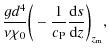
We begin by investigating the linear regime where the magnetic field is still weak. In that case the values of3.1.1 Dependence on Rm
From the perspective of mean-field dynamo theory a,
large-scale dynamo should operate if
![]() .
We start the simulations with a random small-scale magnetic field of
the order of
.
We start the simulations with a random small-scale magnetic field of
the order of
![]() and monitor the time evolution of the total
magnetic field quantified by
and monitor the time evolution of the total
magnetic field quantified by
![]() .
We indeed find that in runs with vertical-field boundary conditions
the dynamo is excited
for
.
We indeed find that in runs with vertical-field boundary conditions
the dynamo is excited
for
![]() ,
whereas in the case of perfectly conducting
boundaries, the critical value is about five times higher (see
Table 1 and Fig. 1).
,
whereas in the case of perfectly conducting
boundaries, the critical value is about five times higher (see
Table 1 and Fig. 1).
As a consistency check we use a one-dimensional mean-field model
written in terms of the vector potential
| (17) |
where
We find a marginal value
![]() for the vertical-field
boundary conditions, whereas in the case of perfect-conductor boundaries
for the vertical-field
boundary conditions, whereas in the case of perfect-conductor boundaries
![]() is obtained. These values are very close to
those obtained from direct simulations, although one must bear in
mind that the
is obtained. These values are very close to
those obtained from direct simulations, although one must bear in
mind that the ![]() -dependence of
-dependence of
![]() and
and ![]() at
small values of
at
small values of ![]() (Käpylä et al. 2009b) is not taken
into account in our mean-field modelling. However, the qualitative
result that the dynamo is harder to excite when perfect-conductor
boundaries are used is consistent with the direct simulations.
(Käpylä et al. 2009b) is not taken
into account in our mean-field modelling. However, the qualitative
result that the dynamo is harder to excite when perfect-conductor
boundaries are used is consistent with the direct simulations.
We measure the growth rate, ![]() ,
of the rms magnetic field as
,
of the rms magnetic field as
| (18) |
where
![\begin{figure}
\par\includegraphics[width=8.8cm,clip]{13722fg1.eps}
\end{figure}](/articles/aa/full_html/2010/10/aa13722-09/img102.png)
|
Figure 1:
Growth rate |
| Open with DEXTER | |
![\begin{figure}
\par\includegraphics[width=8.8cm,clip]{13722fg2.eps}
\end{figure}](/articles/aa/full_html/2010/10/aa13722-09/img103.png)
|
Figure 2:
Growth rate |
| Open with DEXTER | |
![\begin{figure}
\par\includegraphics[width=8.8cm,clip]{13722fg3.eps}
\end{figure}](/articles/aa/full_html/2010/10/aa13722-09/img104.png)
|
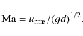
Figure 3:
Dynamo numbers according to Eq. (23) as functions of
rotation for the runs listed in Table 2. The solid
(dashed) curve shows the results for vertical-field
(perfect-conductor) boundary conditions. The horizontal dash-dotted and
dash-triple-dotted lines indicate the critical dynamo number in the
case of open and closed boundaries, respectively. Power law
proportional to
|
| Open with DEXTER | |
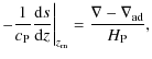
3.1.2 Dependence on shear and rotation
In addition to the dependence on the magnetic Reynolds number,
we study the influence of shear on
the excitation of the dynamo. We use a setup where
![]() in
the case
in
the case
![]() ,
in which case the small-scale dynamo is
marginal. We then introduce shear and rotation into the system and
keep the quantity
,
in which case the small-scale dynamo is
marginal. We then introduce shear and rotation into the system and
keep the quantity
![]() fixed in all cases. Our results
for the growth rate of the magnetic field in the range
fixed in all cases. Our results
for the growth rate of the magnetic field in the range
![]() are shown in Fig. 2. We find
that for a given
are shown in Fig. 2. We find
that for a given ![]() the growth rate is always greater in the
simulations with open boundaries (see also Table 2).
The case
the growth rate is always greater in the
simulations with open boundaries (see also Table 2).
The case
![]() (Run VF11) is very
close to marginal in the case of open boundaries, but clearly
subcritical when perfectly conducting boundaries are used (Run PC9).
The critical value of
(Run VF11) is very
close to marginal in the case of open boundaries, but clearly
subcritical when perfectly conducting boundaries are used (Run PC9).
The critical value of
![]() in the perfect-conductor case seems to be roughly twice as large
as the corresponding value in the vertical-field runs.
To be more precise, we estimate the relevant dynamo numbers as
in the perfect-conductor case seems to be roughly twice as large
as the corresponding value in the vertical-field runs.
To be more precise, we estimate the relevant dynamo numbers as
| |
|
(19) | |
|
(20) |
where
| (21) |
Furthermore, we assume the Strouhal number,
| (22) |
of unity (as found by Brandenburg & Subramanian 2005b) so that
For the marginal open-field Run VF11 we find a critical dynamo number
In the preceding simplified analysis we have estimated
![]() and
and
![]() using volume averages that are not ideally suited
for the present case (see, e.g. Käpylä et al. 2009b). Furthermore, we have assumed here that the dynamo
is of pure
using volume averages that are not ideally suited
for the present case (see, e.g. Käpylä et al. 2009b). Furthermore, we have assumed here that the dynamo
is of pure ![]() -shear type and have neglected all other possible
induction
effects (shear-current,
-shear type and have neglected all other possible
induction
effects (shear-current,
![]() ,
and incoherent
,
and incoherent
![]() -shear effects) that can assist in dynamo action
(Käpylä et al. 2009b). This means that
the quantitative results should be taken with some amount of caution.
-shear effects) that can assist in dynamo action
(Käpylä et al. 2009b). This means that
the quantitative results should be taken with some amount of caution.
In Paper I, the only case where open and closed boundaries were compared
was the one where only shear was present, i.e.
![]() ,
whereas
,
whereas
![]() (Run C
with vertical-field boundary conditions versus Run C' with
perfect-conductor boundary conditions). In
Paper I we also showed that, in the absence of rotation, the growth rate
of the magnetic field is reduced in comparison to the case where
both shear and rotation are present. Furthermore, our present results
suggest that the
large-scale dynamo is harder to excite in the case of
perfect-conductor boundaries. Thus, a reasonable explanation to the
slow growth of
the large-scale field in Run C' of Paper I is that the system is
close to being marginally excited, and not, as suggested by Hughes
& Proctor (2009), the result of some nonlinear effect
arising from magnetic helicity flux out of the system.
A straightforward quantitative analysis in terms of a
classical
(Run C
with vertical-field boundary conditions versus Run C' with
perfect-conductor boundary conditions). In
Paper I we also showed that, in the absence of rotation, the growth rate
of the magnetic field is reduced in comparison to the case where
both shear and rotation are present. Furthermore, our present results
suggest that the
large-scale dynamo is harder to excite in the case of
perfect-conductor boundaries. Thus, a reasonable explanation to the
slow growth of
the large-scale field in Run C' of Paper I is that the system is
close to being marginally excited, and not, as suggested by Hughes
& Proctor (2009), the result of some nonlinear effect
arising from magnetic helicity flux out of the system.
A straightforward quantitative analysis in terms of a
classical ![]() -shear dynamo described above is, however, not useful in the
non-rotating case. This is shown by the results of Käpylä et al. (2009b): the main contribution to dynamo action in this
case is due to the incoherent
-shear dynamo described above is, however, not useful in the
non-rotating case. This is shown by the results of Käpylä et al. (2009b): the main contribution to dynamo action in this
case is due to the incoherent ![]() -shear process which relies on
the fluctuations of
-shear process which relies on
the fluctuations of ![]() (e.g. Vishniac & Brandenburg
1997; Sokolov 1997; Silant'ev 2000; Proctor
2007).
(e.g. Vishniac & Brandenburg
1997; Sokolov 1997; Silant'ev 2000; Proctor
2007).
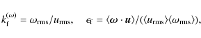
![\begin{figure}
\par\includegraphics[width=17cm,clip]{13722fg4.eps}
\end{figure}](/articles/aa/full_html/2010/10/aa13722-09/img130.png)
|
Figure 4:
Magnetic field component By from runs with vertical-field
( left column) and perfect-conductor ( right column) boundary
conditions. Three different cases with low ( top), intermediate
( middle) and high ( bottom) |
| Open with DEXTER | |
![\begin{figure}
\par\includegraphics[width=16cm,clip]{13722fg5.eps}
\vspace{-2mm}\end{figure}](/articles/aa/full_html/2010/10/aa13722-09/img131.png)
|
Figure 5:
Horizontally averaged magnetic field components Bx and
By from the same six runs as in Fig. 4.
Those runs and the corresponding values of |
| Open with DEXTER | |
3.2 Nonlinear regime
We find that in all cases where a dynamo is excited, large-scale
magnetic fields are also generated. In the low-![]() runs the
large-scale contribution is substantial, i.e.
runs the
large-scale contribution is substantial, i.e.
![]() is
close to unity already in the kinematic
regime. In the cases where also the fluctuation dynamo is
excited, a large-scale pattern is discernible only
once the dynamo has reached saturation.
This feature is common to all known large-scale dynamos
and was already seen in simulations of Brandenburg (2001).
Figure 4 shows visualizations of
the streamwise component of the field in the saturated state for three Reynolds
numbers, representing low, intermediate, and
high
is
close to unity already in the kinematic
regime. In the cases where also the fluctuation dynamo is
excited, a large-scale pattern is discernible only
once the dynamo has reached saturation.
This feature is common to all known large-scale dynamos
and was already seen in simulations of Brandenburg (2001).
Figure 4 shows visualizations of
the streamwise component of the field in the saturated state for three Reynolds
numbers, representing low, intermediate, and
high ![]() ,
with open and closed boundaries (see Table 1).
The runs depicted in Fig. 4 are indicated in boldface
in the table.
Although an increasing amount of
small-scale features is seen with increasing
,
with open and closed boundaries (see Table 1).
The runs depicted in Fig. 4 are indicated in boldface
in the table.
Although an increasing amount of
small-scale features is seen with increasing ![]() ,
a large-scale
pattern is clearly visible in all cases.
,
a large-scale
pattern is clearly visible in all cases.
Unlike the case with just rotation and no shear,
where the mean field shows variations in the horizontal directions
(Käpylä et al. 2009a), here the kx=ky=0 mode
dominates the large-scale field and thus horizontal averages are
suitable. Space-time diagrams of the horizontally averaged magnetic
field components,
![]() and
and
![]() ,
are shown in
Fig. 5 for the same runs as in Fig. 4.
We find that the large-scale field is non-oscillatory in all cases,
which is in agreement with earlier results (Paper I; Hughes &
Proctor 2009; Käpylä et al. 2010).
In most cases, regardless of the
boundary conditions, the field changes sign near the base of the
convectively unstable layer, with the exception of the runs with
vertical-field boundary conditions (VF runs) with the lowest values of
,
are shown in
Fig. 5 for the same runs as in Fig. 4.
We find that the large-scale field is non-oscillatory in all cases,
which is in agreement with earlier results (Paper I; Hughes &
Proctor 2009; Käpylä et al. 2010).
In most cases, regardless of the
boundary conditions, the field changes sign near the base of the
convectively unstable layer, with the exception of the runs with
vertical-field boundary conditions (VF runs) with the lowest values of ![]() .
(The solutions are invariant under sign reversal,
.
(The solutions are invariant under sign reversal,
![]() ,
and
both realizations of the large-scale field are found in Figs. 4
and 5, depending just on the initial conditions.)
In the perfect-conductor runs (PC runs), the
field near the top of the domain has a different sign than in the bulk
of the convection zone, whereas in the VF runs such
behaviour is not seen.
We find that in the PC runs the layer of oppositely
directed field becomes progressively thinner as
,
and
both realizations of the large-scale field are found in Figs. 4
and 5, depending just on the initial conditions.)
In the perfect-conductor runs (PC runs), the
field near the top of the domain has a different sign than in the bulk
of the convection zone, whereas in the VF runs such
behaviour is not seen.
We find that in the PC runs the layer of oppositely
directed field becomes progressively thinner as ![]() is increased,
leading to strong gradients near the boundary (see
Fig. 5). This can possibly explain the numerical
problems encountered in the
is increased,
leading to strong gradients near the boundary (see
Fig. 5). This can possibly explain the numerical
problems encountered in the
![]() simulation (Run PC9) with
perfect-conductor boundary conditions.
The saturated state of Run PC9 is significantly shorter
than that of the other runs due to numerical instability that
prevented running the simulation further.
simulation (Run PC9) with
perfect-conductor boundary conditions.
The saturated state of Run PC9 is significantly shorter
than that of the other runs due to numerical instability that
prevented running the simulation further.
It turns out that the emergence of the large-scale field occurs
progressively earlier as ![]() is increased.
This can be seen most clearly in Fig. 5, which shows that
the large-scale field has reached saturation in less than 200 turnover times
for
is increased.
This can be seen most clearly in Fig. 5, which shows that
the large-scale field has reached saturation in less than 200 turnover times
for
![]() (Run VF10), while for Runs VF7 and VF4 with
(Run VF10), while for Runs VF7 and VF4 with
![]() and 3.7, the saturation times exceed 300 and 400 turnover times, respectively.
A similar trend is seen also in the PC runs.
In an earlier study we found that the mean values of the turbulent
transport coefficients relevant for the generation of large-scale
magnetic fields,
and 3.7, the saturation times exceed 300 and 400 turnover times, respectively.
A similar trend is seen also in the PC runs.
In an earlier study we found that the mean values of the turbulent
transport coefficients relevant for the generation of large-scale
magnetic fields,
![]() and
and
![]() ,
remain constant within the
errors given that
,
remain constant within the
errors given that
![]() ;
see Fig. 5 of Käpylä et al. (2009b). However, as the magnetic Reynolds number is
increased, the fluctuations of
;
see Fig. 5 of Käpylä et al. (2009b). However, as the magnetic Reynolds number is
increased, the fluctuations of ![]() tend to increase as well. Such
fluctuations can contribute to the incoherent
tend to increase as well. Such
fluctuations can contribute to the incoherent ![]() -shear process
which can possibly explain the faster saturation of the large-scale
field when
-shear process
which can possibly explain the faster saturation of the large-scale
field when ![]() is increased.
is increased.
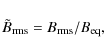
The saturation level of the total and mean magnetic fields for runs
with open and
closed boundary conditions are shown in Fig. 6.
We find that the total magnetic field in the runs with open boundary
conditions is roughly consistent with an ![]() -independent value. In
the perfect-conductor case the total magnetic energy first increases
up to
-independent value. In
the perfect-conductor case the total magnetic energy first increases
up to
![]() and then decreases
proportionally to
and then decreases
proportionally to
![]() for
for
![]() .
Mean-field models taking
into account magnetic helicity evolution can also produce a maximum
for the saturation level at some intermediate
.
Mean-field models taking
into account magnetic helicity evolution can also produce a maximum
for the saturation level at some intermediate ![]() (e.g. Brandenburg
et al. 2007). We note that an
(e.g. Brandenburg
et al. 2007). We note that an
![]() dependence for the
mean field energy is indicative of catastrophic quenching. This would indeed
be the expected result for closed boundaries. However, in our case
only the total field energy shows the
dependence for the
mean field energy is indicative of catastrophic quenching. This would indeed
be the expected result for closed boundaries. However, in our case
only the total field energy shows the
![]() behaviour whereas
the mean field
exhibits a much steeper (at least
behaviour whereas
the mean field
exhibits a much steeper (at least
![]() )
dependence. The
explanation for such a steep trend is as yet unclear. The data for the
mean magnetic field in the case of open boundaries also show a weak
decreasing trend consistent with a power law
)
dependence. The
explanation for such a steep trend is as yet unclear. The data for the
mean magnetic field in the case of open boundaries also show a weak
decreasing trend consistent with a power law
![]() as opposed to the expectation that the
saturation level is independent of
as opposed to the expectation that the
saturation level is independent of ![]() .
However, the unexpected behaviour of the saturation level could simply
be related to the fact that in mean-field models
true asymptotic behaviour may only commence at much larger values of
.
However, the unexpected behaviour of the saturation level could simply
be related to the fact that in mean-field models
true asymptotic behaviour may only commence at much larger values of ![]() (Brandenburg et al. 2009).
(Brandenburg et al. 2009).
Our simulations with the highest magnetic Reynolds numbers
and closed boundaries apparently do not
show a slow saturation behaviour; e.g. as in Fig. 7 where the
mean magnetic field and a saturation predictor (Brandenburg
2001) proportional to
![]() are shown
for Runs PC6-PC8.
Here we use
are shown
for Runs PC6-PC8.
Here we use
![]() and
and
![]() is the time at
which the small-scale dynamo has saturated.
In the runs with intermediate
is the time at
which the small-scale dynamo has saturated.
In the runs with intermediate ![]() (PC6 and PC7) the saturation predictor
is in fairly good agreement with the simulation results, whereas for
Run PC8 this is no longer the case.
This might be caused by additional contributions to
(PC6 and PC7) the saturation predictor
is in fairly good agreement with the simulation results, whereas for
Run PC8 this is no longer the case.
This might be caused by additional contributions to
![]() whose effective value of k is larger.
In fact, earlier simulations of forced turbulence with perfect-conductor
boundary conditions (Brandenburg & Dobler 2002) showed that the
final configuration of the mean field can be established in steps,
but the time between different steps can still be resistively long.
This could explain why, in the highest-
whose effective value of k is larger.
In fact, earlier simulations of forced turbulence with perfect-conductor
boundary conditions (Brandenburg & Dobler 2002) showed that the
final configuration of the mean field can be established in steps,
but the time between different steps can still be resistively long.
This could explain why, in the highest-![]() simulations, the
saturation level of the
mean magnetic field is lower than expected.
Whether this is also the case in the present simulations remains an
open question.
simulations, the
saturation level of the
mean magnetic field is lower than expected.
Whether this is also the case in the present simulations remains an
open question.
![\begin{figure}
\par\includegraphics[width=8.5cm,clip]{13722fg6.eps}
\end{figure}](/articles/aa/full_html/2010/10/aa13722-09/img146.png)
|
Figure 6:
Upper panel: rms-value of the total magnetic field in the
saturated regime for runs with perfect-conductor (solid line) and
vertical-field (dashed) boundaries. Lower panel: same as above but
for the horizontally averaged mean magnetic field
|
| Open with DEXTER | |
![\begin{figure}
\par\includegraphics[width=8.5cm,clip]{13722fg7.eps}
\end{figure}](/articles/aa/full_html/2010/10/aa13722-09/img147.png)
|
Figure 7:
Mean magnetic field as a function of time from Runs PC6 (solid
line), and PC7 (dashed). The inset shows the same for Run PC8.
The dotted lines show a saturation
predictor according to Brandenburg (2001) with the
microscopic values of |
| Open with DEXTER | |
4 Conclusions
We have studied the effects of magnetic boundary conditions on the excitation and saturation of large-scale dynamos driven by turbulent convection, shear, and rotation by means of numerical simulations. We find that the critical magnetic Reynolds number is greater (The measured growth rate of the magnetic field is independent of the
microscopic resistivity when ![]() is sufficiently above the
critical value. This is manifested by the approximately constant
growth rate in the intermediate
is sufficiently above the
critical value. This is manifested by the approximately constant
growth rate in the intermediate ![]() range in Fig. 1.
For
range in Fig. 1.
For
![]() ,
the small-scale dynamo is excited, and for
,
the small-scale dynamo is excited, and for
![]() it becomes dominant. The growth rate of the magnetic
field is then consistent with
it becomes dominant. The growth rate of the magnetic
field is then consistent with
![]() scaling, which is in
accordance with the results of Schekochihin et al. (2004)
and Haugen et al. (#HBD04<#916). The fact that the qualitative
behaviour of the growth rate of the magnetic field is similar for both
boundary conditions suggests that the origin of the large-scale dynamo is not
likely to be a process that is essentially nonlinear, as suggested by
Hughes & Proctor (2009), but that it can be understood within
the framework of classical kinematic mean-field theory.
scaling, which is in
accordance with the results of Schekochihin et al. (2004)
and Haugen et al. (#HBD04<#916). The fact that the qualitative
behaviour of the growth rate of the magnetic field is similar for both
boundary conditions suggests that the origin of the large-scale dynamo is not
likely to be a process that is essentially nonlinear, as suggested by
Hughes & Proctor (2009), but that it can be understood within
the framework of classical kinematic mean-field theory.
In the saturated state the energy of the total magnetic field remains
independent of ![]() for
open boundaries and decreases as
for
open boundaries and decreases as
![]() for closed
boundaries. The
latter result is consistent with catastrophic quenching while the former
result suggests that magnetic helicity fluxes are efficiently driven
out of the system.
On the other hand, the energy of the mean field, taken here to be
represented by horizontal averages, decreases approximately as
for closed
boundaries. The
latter result is consistent with catastrophic quenching while the former
result suggests that magnetic helicity fluxes are efficiently driven
out of the system.
On the other hand, the energy of the mean field, taken here to be
represented by horizontal averages, decreases approximately as
![]() for
open and as
for
open and as
![]() for closed boundaries. It is not yet
clear why the mean fields tend to show a steeper decline than the total
field. It is possible that this declining trend levels off at a higher
for closed boundaries. It is not yet
clear why the mean fields tend to show a steeper decline than the total
field. It is possible that this declining trend levels off at a higher ![]() and
that the magnetic Reynolds numbers in our simulations are still not
large enough
(cf. Brandenburg et al. 2009). A similarly weak
and
that the magnetic Reynolds numbers in our simulations are still not
large enough
(cf. Brandenburg et al. 2009). A similarly weak
![]() -dependence has been observed in the cycle period of
-dependence has been observed in the cycle period of
![]() -shear dynamos with isotropically forced turbulence
(Käpylä & Brandenburg 2009).
-shear dynamos with isotropically forced turbulence
(Käpylä & Brandenburg 2009).
We find that, for intermediate values of ![]() ,
the large-scale
magnetic field
saturates on a resistive time scale when closed boundaries are used.
However, with the largest
,
the large-scale
magnetic field
saturates on a resistive time scale when closed boundaries are used.
However, with the largest ![]() no clear signs of slow saturation are
observed. Earlier results using perfect-conductor boundaries have
shown that the mean field can evolve in steps (Brandenburg & Dobler
2002; see also Brandenburg et al. 2007) which are
associated with a change of the large-scale magnetic field
configuration. We have not seen such a behaviour in our current
simulations but the existence of such events at a later stage cannot
be ruled out. Another possible explanation is that there are magnetic
helicity fluxes
occurring inside the domain which arise from the spatial gradients of
magnetic helicity (e.g. Covas et al. 1998;
Kleeorin et al. 2000; Mitra et al. 2010).
However, a quantitative study of these effects requires more detailed
knowledge of the helicity fluxes and possibly an anisotropic formulation of the
magnetic
no clear signs of slow saturation are
observed. Earlier results using perfect-conductor boundaries have
shown that the mean field can evolve in steps (Brandenburg & Dobler
2002; see also Brandenburg et al. 2007) which are
associated with a change of the large-scale magnetic field
configuration. We have not seen such a behaviour in our current
simulations but the existence of such events at a later stage cannot
be ruled out. Another possible explanation is that there are magnetic
helicity fluxes
occurring inside the domain which arise from the spatial gradients of
magnetic helicity (e.g. Covas et al. 1998;
Kleeorin et al. 2000; Mitra et al. 2010).
However, a quantitative study of these effects requires more detailed
knowledge of the helicity fluxes and possibly an anisotropic formulation of the
magnetic ![]() effect. These issues merit further investigation and
are beyond the scope of the present paper.
effect. These issues merit further investigation and
are beyond the scope of the present paper.
The authors thank Anvar Shukurov for his detailed comments on the paper. The computations were performed on the facilities hosted by the CSC - IT Center for Science in Espoo, Finland, administered by the Finnish ministry of education. We also wish to acknowledge the DECI - DEISA network for granting computational resources to the CONVDYN project. Financial support from the Academy of Finland grants No. 121431 (PJK) and 112020 (MJK), as well as the Swedish Research Council grant 621-2007-4064 and the European Research Council AstroDyn Research Project 227952 (AB) are acknowledged. The authors acknowledge the hospitality of Nordita during the program ``Solar and stellar dynamos and cycles''.
References
- Blackman, E. G., & Field, G. B. 2000, ApJ, 534, 984 [NASA ADS] [CrossRef] [Google Scholar]
- Brandenburg, A. 2001, ApJ, 550, 824 [NASA ADS] [CrossRef] [Google Scholar]
- Brandenburg, A. 2005, ApJ, 625, 539 [Google Scholar]
- Brandenburg, A., & Dobler, W. 2002, Comp. Phys. Comm., 147, 471 [Google Scholar]
- Brandenburg, A., & Sandin, C. 2004, A&A, 427, 13 [NASA ADS] [CrossRef] [EDP Sciences] [Google Scholar]
- Brandenburg, A., & Subramanian, K. 2005a, AN, 326, 400 [Google Scholar]
- Brandenburg, A., & Subramanian, K. 2005b, A&A, 439, 835 [NASA ADS] [CrossRef] [EDP Sciences] [Google Scholar]
- Brandenburg, A., Käpylä, P. J., Mitra, D., Moss, D., & Tavakol, R. 2007, AN, 328, 1118 [NASA ADS] [Google Scholar]
- Brandenburg, A., Rädler, K.-H., Rheinhardt, M., & Käpylä, P. J. 2008, ApJ, 676, 740 [NASA ADS] [CrossRef] [Google Scholar]
- Brandenburg, A., Candelaresi, S., & Chatterjee, P. 2009, MNRAS, 398, 1414 [NASA ADS] [CrossRef] [Google Scholar]
- Cattaneo, F., & Hughes, D. W. 1996, PhRvE, 54, R4532 [Google Scholar]
- Choudhuri, A. R. 1984, ApJ, 281, 846 [NASA ADS] [CrossRef] [Google Scholar]
- Covas, E., Tavakol, R., Tworkowski, A., & Brandenburg, A. 1998, A&A, 329, 350 [NASA ADS] [Google Scholar]
- Haugen, N. E. L., Brandenburg, A., & Dobler, W. 2004, PhRvE, 70, 016308 [NASA ADS] [Google Scholar]
- Hughes, D. W., & Proctor, M. R. E. 2009, PhRvL, 102, 044501 [Google Scholar]
- Jouve, L., Brun, A. S., Arlt, R., et al. 2008, A&A, 483, 949 [NASA ADS] [CrossRef] [EDP Sciences] [Google Scholar]
- Käpylä, P. J., & Brandenburg, A. 2009, ApJ, 699, 1059 [NASA ADS] [CrossRef] [Google Scholar]
- Käpylä, P. J., Korpi, M. J., & Brandenburg, A. 2008, A&A, 491, 353 (Paper I) [NASA ADS] [CrossRef] [EDP Sciences] [Google Scholar]
- Käpylä, P. J., Korpi, M. J., & Brandenburg, A. 2009a, ApJ, 697, 1153 [NASA ADS] [CrossRef] [Google Scholar]
- Käpylä, P. J., Korpi, M. J., & Brandenburg, A. 2009b, A&A, 500, 633 [NASA ADS] [CrossRef] [EDP Sciences] [Google Scholar]
- Käpylä, P. J., Korpi, M. J., & Brandenburg, A. 2010, MNRAS, 402, 1458 [NASA ADS] [CrossRef] [Google Scholar]
- Kleeorin, N., Moss, D., Rogachevskii, I., &Sokoloff, D. 2000, A&A, 361, L5 [NASA ADS] [Google Scholar]
- Krause, F., & Rädler, K.-H. 1980, Mean-field Magnetohydrodynamics and Dynamo Theory (Oxford: Pergamon Press) [Google Scholar]
- Mitra, D., Candelaresi, S., Chatterjee, P., Tavakol, R., & Brandenburg, A. 2010, AN, 331, 130 [Google Scholar]
- Moffatt, H. K. 1978, Magnetic field generation in electrically conducting fluids (Cambridge: Cambridge Univ. Press) [Google Scholar]
- Parker, E. N. 1955, ApJ, 122, 293 [NASA ADS] [CrossRef] [Google Scholar]
- Parker, E. N. 1979, Cosmical Magnetic Fields: Their Origin and Their Activity (Oxford & NY: Clarendon Press) [Google Scholar]
- Proctor, M. R. E. 2007, MNRAS, 382, 39 [NASA ADS] [CrossRef] [Google Scholar]
- Rüdiger, G., & Hollerbach, R. 2004, The Magnetic Universe (Weinheim: Wiley-VCH) [Google Scholar]
- Schekochihin, A. A., Cowley, S. C., Taylor, S. F., Maron, J. L., & McWilliams, J. C. 2004, ApJ, 612, 276 [NASA ADS] [CrossRef] [Google Scholar]
- Silant'ev, N. A.. 2000, A&A, 364, 339 [NASA ADS] [Google Scholar]
- Sokolov, D. D. 1997, Astron. Rep., 41, 68 [NASA ADS] [Google Scholar]
- Steenbeck, M., & Krause, F. 1969, AN, 291, 49 [Google Scholar]
- Tobias, S. M., Cattaneo, F., & Brummell, N. H. 2008, ApJ, 685, 596 [NASA ADS] [CrossRef] [Google Scholar]
- Vainshtein, S. I., & Cattaneo, F. 1992, ApJ, 393, 165 [NASA ADS] [CrossRef] [Google Scholar]
- Vishniac, E. T., & Brandenburg, A. 1997, ApJ, 475, 263 [NASA ADS] [CrossRef] [Google Scholar]
- Vishniac, E. T., & Cho, J. 2001, ApJ, 550, 752 [NASA ADS] [CrossRef] [Google Scholar]
- Wisdom, J., & Tremaine, S. 1988, AJ, 95, 925 [NASA ADS] [CrossRef] [Google Scholar]
- Yousef, T. A., Heinemann, T., Schekochihin, A. A., et al. 2008a, PhRvL, 100, 184501 [NASA ADS] [CrossRef] [PubMed] [Google Scholar]
- Yousef, T. A., Heinemann, T., Rincon, F., et al. 2008b, AN, 329, 737 [NASA ADS] [CrossRef] [Google Scholar]
Footnotes
All Tables
Table 1:
Summary of the runs with varying ![]() .
.
Table 2:
Summary of the runs with varying ![]() and
and ![]() .
.
All Figures
|
|
Figure 1:
Growth rate |
| Open with DEXTER | |
| In the text | |
|
|
Figure 2:
Growth rate |
| Open with DEXTER | |
| In the text | |
|
|
Figure 3:
Dynamo numbers according to Eq. (23) as functions of
rotation for the runs listed in Table 2. The solid
(dashed) curve shows the results for vertical-field
(perfect-conductor) boundary conditions. The horizontal dash-dotted and
dash-triple-dotted lines indicate the critical dynamo number in the
case of open and closed boundaries, respectively. Power law
proportional to
|
| Open with DEXTER | |
| In the text | |
|
|
Figure 4:
Magnetic field component By from runs with vertical-field
( left column) and perfect-conductor ( right column) boundary
conditions. Three different cases with low ( top), intermediate
( middle) and high ( bottom) |
| Open with DEXTER | |
| In the text | |
|
|
Figure 5:
Horizontally averaged magnetic field components Bx and
By from the same six runs as in Fig. 4.
Those runs and the corresponding values of |
| Open with DEXTER | |
| In the text | |
|
|
Figure 6:
Upper panel: rms-value of the total magnetic field in the
saturated regime for runs with perfect-conductor (solid line) and
vertical-field (dashed) boundaries. Lower panel: same as above but
for the horizontally averaged mean magnetic field
|
| Open with DEXTER | |
| In the text | |
|
|
Figure 7:
Mean magnetic field as a function of time from Runs PC6 (solid
line), and PC7 (dashed). The inset shows the same for Run PC8.
The dotted lines show a saturation
predictor according to Brandenburg (2001) with the
microscopic values of |
| Open with DEXTER | |
| In the text | |
Copyright ESO 2010
Current usage metrics show cumulative count of Article Views (full-text article views including HTML views, PDF and ePub downloads, according to the available data) and Abstracts Views on Vision4Press platform.
Data correspond to usage on the plateform after 2015. The current usage metrics is available 48-96 hours after online publication and is updated daily on week days.
Initial download of the metrics may take a while.