| Issue |
A&A
Volume 518, July-August 2010
Herschel: the first science highlights
|
|
|---|---|---|
| Article Number | A21 | |
| Number of page(s) | 10 | |
| Section | Cosmology (including clusters of galaxies) | |
| DOI | https://doi.org/10.1051/0004-6361/200913581 | |
| Published online | 25 August 2010 | |
A (giant) void is not mandatory to explain away dark energy with a Lemaître-Tolman model
M.-N. Célérier1 - K. Bolejko2,3 - A. Krasinski3
1 - Laboratoire Univers et Théories (LUTH),
Observatoire de Paris, CNRS, Université Paris-Diderot, 5 place Jules
Janssen, 92190 Meudon, France
2 -
Department
of Mathematics and Applied Mathematics, University of Cape Town, Rondebosch 7701, South Africa
3 -
Nicolaus Copernicus Astronomical Centre, Polish Academy of Sciences, Bartycka 18, 00 716 Warszawa, Poland
Received 2 November 2009 / Accepted 3 May 2010
Abstract
Context. Lemaître-Tolman (L-T) toy models with a central
observer have been used to study the effect of large scale
inhomogeneities on the SN Ia dimming. Claims that a giant void is
mandatory to explain away dark energy in this framework are currently
dominating.
Aims. Our aim is to show that L-T models exist that reproduce a few features of the ![]() CDM model, but do not contain the giant cosmic void.
CDM model, but do not contain the giant cosmic void.
Methods. We propose to use two sets of data - the angular
diameter distance together with the redshift-space mass-density and the
angular diameter distance together with the expansion rate - both
defined on the past null cone as functions of the redshift. We assume
that these functions are of the same form as in the ![]() CDM
model. Using the Mustapha-Hellaby-Ellis algorithm, we numerically
transform these initial data into the usual two L-T arbitrary functions
and solve the evolution equation to calculate the mass distribution in
spacetime.
CDM
model. Using the Mustapha-Hellaby-Ellis algorithm, we numerically
transform these initial data into the usual two L-T arbitrary functions
and solve the evolution equation to calculate the mass distribution in
spacetime.
Results. For both models, we find that the current density
profile does not exhibit a giant void, but rather a giant hump.
However, this hump is not directly observable, since it is in a
spacelike relation to a present observer.
Conclusions. The alleged existence of the giant void was a
consequence of the L-T models used earlier because their generality was
limited a priori by needless simplifying assumptions, like, for
example, the bang-time function being constant. Instead, one can feed
any mass distribution or expansion rate history on the past light cone
as initial data to the L-T evolution equation. When a fully general L-T
metric is used, the giant void is not implied.
Key words: cosmology: dark energy - cosmology: miscellaneous
1 The historical background of the problem
In the framework of the homogeneous and isotropic standard cosmological model, the dimming of the type Ia supernovae as compared to their expected luminosity in an Einstein-de Sitter model is interpreted as a consequence of an assumed accelerated expansion of the Universe. This leads to the widespread belief in a ``dark energy'' component currently dominating the energy budget of our Universe. But this is not the only possible explanation of the SN Ia observations.
Shortly after the discovery by Riess et al. (1998) and Perlmutter et al. (1999) of the supernova dimming, it was proposed by several authors that this effect could be due to the large-scale inhomogeneities (Pascual-Sánchez 1999; Célérier 2000; Tomita 2000, 2001a,b). After a period of relative disaffection, this proposal experienced a renewed interest about five years ago.
Three methods have been used to implement such a proposal: computation of backreaction terms in the dynamical equations using an averaging procedure proposed by Buchert (2000, 2001), calculations in the framework of a perturbative scheme and the use of exact inhomogeneous models, in particular those of Lemaître (1933) - Tolman (1934) (L-T) (see Célérier 2007, for a review).
The L-T model became rapidly popular for the purpose of mimicking ``dark energy''
because it exhibits three interesting features: i) it is one of the few exact
solutions of General Relativity able to represent a physically consistent model
of the matter dominated era of the Universe; ii) among these few, it is the most
easily tractable from a computational point of view;
iii) it is not an alternative to, but a generalisation of the Friedmann
dust models (which are contained in it as a subcase), so can reproduce all the
Friedmann-based results, including those of the ``concordance'' ![]() CDM
model, with an arbitrary precision. For more on this, in relation to the main
subject of this paper, see the last section.
CDM
model, with an arbitrary precision. For more on this, in relation to the main
subject of this paper, see the last section.
Three classes of models have been constructed with the L-T solution: i) models
where the observer is located at the centre of a single L-T universe (e.g.,
Iguchi et al. 2002; Alnes et al. 2006; Apostolopoulos et al.
2006; Bolejko 2008; Garcia-Bellido & Haugbølle 2008a, 2009); ii) models where
the observer is located off the centre of such a universe (e.g., Schneider &
Célérier 1999; Apostolopoulos et al. 2006; Alnes & Amarzguioui 2007)![]() ; iii)
Swiss-cheese models where the holes are L-T bubbles carved out of a
Friedmannian homogeneous background (e.g., Brouzakis et al. 2007, 2008; Biswas & Notari 2008; Marra et al. 2007).
; iii)
Swiss-cheese models where the holes are L-T bubbles carved out of a
Friedmannian homogeneous background (e.g., Brouzakis et al. 2007, 2008; Biswas & Notari 2008; Marra et al. 2007).
As will be recalled in Sect. 2, an L-T model is defined by two independent arbitrary functions of the radial coordinate, which can be fitted to the observational data. However, in most of the models currently available in the literature, the authors have artificially limited the generality by giving the L-T initial-data functions a handpicked algebraic form (depending on the authors' feelings about which kind of model would best represent our Universe), with only a few constant parameters being left arbitrary - to be adapted to the observations.
Another way in which the generality of the L-T models was artificially
limited was the assumption that the age of the Universe is everywhere the same,
i.e. that the L-T bang-time function ![]() is constant. With
is constant. With ![]() being
constant, the only single-patch L-T model that fits observations is one with a
giant void (Iguchi et al. 2002; Yoo et al. 2008). Conceptually there
is nothing wrong with a non-simultaneous big bang (even though this is a radical
qualitative difference with the FLRW models), but one should exercise caution
when referring to
being
constant, the only single-patch L-T model that fits observations is one with a
giant void (Iguchi et al. 2002; Yoo et al. 2008). Conceptually there
is nothing wrong with a non-simultaneous big bang (even though this is a radical
qualitative difference with the FLRW models), but one should exercise caution
when referring to
![]() as the actual age of the Universe. The L-T model
is too simple to extend it up to instants earlier than decoupling. Therefore
as the actual age of the Universe. The L-T model
is too simple to extend it up to instants earlier than decoupling. Therefore
![]() should merely be regarded as a function that describes a degree of
inhomogeneity of the initial conditions rather than as the actual instant of
birth of the Universe.
should merely be regarded as a function that describes a degree of
inhomogeneity of the initial conditions rather than as the actual instant of
birth of the Universe.
The argument brought in defense of the constant ![]() assumption is this: a
non-constant
assumption is this: a
non-constant ![]() generates decreasing modes of perturbation of the metric
(Silk 1977; Plebanski & Krasinski 2006), so any substantial
inhomogeneity at the present time stemming from
generates decreasing modes of perturbation of the metric
(Silk 1977; Plebanski & Krasinski 2006), so any substantial
inhomogeneity at the present time stemming from
![]() would imply
``huge'' perturbations of homogeneity at the last scattering. This, in turn, would
contradict the CMB observations and the implications of inflationary models (we
deliberately do not give references here, to avoid blaming any single individual
for what seems to be a piece of conventional wisdom). However, these are only
expectations that should not be treated as objective truth until they are
verified by calculations. Such calculations have already been done, and it
turned out that the inhomogeneities in
would imply
``huge'' perturbations of homogeneity at the last scattering. This, in turn, would
contradict the CMB observations and the implications of inflationary models (we
deliberately do not give references here, to avoid blaming any single individual
for what seems to be a piece of conventional wisdom). However, these are only
expectations that should not be treated as objective truth until they are
verified by calculations. Such calculations have already been done, and it
turned out that the inhomogeneities in ![]() needed to explain the formation of
galaxy clusters and voids are of the order of a few hundred years (Bolejko
et al. 2005; Krasinski & Hellaby 2004; Bolejko 2009). Then, on the basis
of Bolejko's (2009) models 4 and 5, one can calculate that for a structure of
present radius 30 Mpc this age difference between the oldest and youngest region
would generate CMB temperature fluctuations equal to
needed to explain the formation of
galaxy clusters and voids are of the order of a few hundred years (Bolejko
et al. 2005; Krasinski & Hellaby 2004; Bolejko 2009). Then, on the basis
of Bolejko's (2009) models 4 and 5, one can calculate that for a structure of
present radius 30 Mpc this age difference between the oldest and youngest region
would generate CMB temperature fluctuations equal to
![]() and
and
![]() ,
respectively. This is
well-hidden in the observational errors at the present level of precision. (In
the future, when, presumably, the precision will improve, these results may
possibly be used to measure the gradient of
,
respectively. This is
well-hidden in the observational errors at the present level of precision. (In
the future, when, presumably, the precision will improve, these results may
possibly be used to measure the gradient of ![]() .) So there is no
observational justification to the assumption
.) So there is no
observational justification to the assumption ![]() = constant.
= constant.
These are the reasons why, in the recent years, we have seen the increase in popularity of void models, where the observer is located at or near the centre of a large, huge, giant L-T void of size of up to a few Gpc. Many authors have constructed classes of L-T models with a central local void and have shown that they were able to fit the SN Ia and other cosmological data provided the void is large (e.g., it has a diameter of 400 h-1 Mpc in Alexander et al. 2009) or even huge (e.g., 1.35 Gpc in Alnes et al. 2006, >2 Gpc in Garcia-Bellido & Haugbølle 2008a and 2009), depending on the features of the particular model they had chosen. This contributed to the spreading of the belief in the necessity of a ``giant local void'' to resolve the ``cosmological constant problem'' with L-T models. However, as shown by Mustapha et al. (1998) and used as an illustration for the application to the supernova data and the ``cosmological constant problem'' by Célérier (2000), a given set of isotropic data can constrain only one of the two free functions of an L-T model and therefore, after fitting the supernova data with a given L-T solution, we are left with plenty of room to accommodate more observations.
Actually, a few authors discarded the central void hypothesis and proposed models with no
such void (e.g., Iguchi et al. 2002). Enqvist & Mattsson (2007) even showed that the fitting of the SN Ia data can be better
with L-T models where the density distribution is constant on a constant-time
hypersurface than with the ![]() CDM model (see also Bolejko 2008; Bolejko
& Wyithe 2009). Even though such a density distribution is not what is actually
observed at very large scales by astronomers (it is not even observable, being
in a spacelike relation to the central observer), the
CDM model (see also Bolejko 2008; Bolejko
& Wyithe 2009). Even though such a density distribution is not what is actually
observed at very large scales by astronomers (it is not even observable, being
in a spacelike relation to the central observer), the
![]() const.
configuration vividly illustrates how misleading the FLRW-based geometrical
intuitions can be. A spatial distribution of matter can radically change with
time in consequence of an inhomogeneous expansion distribution in space. Our
models will provide more examples of this phenomenon, and we will come back to
this point in the conclusion.
const.
configuration vividly illustrates how misleading the FLRW-based geometrical
intuitions can be. A spatial distribution of matter can radically change with
time in consequence of an inhomogeneous expansion distribution in space. Our
models will provide more examples of this phenomenon, and we will come back to
this point in the conclusion.
Our aim here is to show, using two explicit examples reproducing the
observational features of the ![]() CDM model, that
a giant void is not at all a necessary implication
of using L-T models. We propose to use input functions that can be derived from
observations
CDM model, that
a giant void is not at all a necessary implication
of using L-T models. We propose to use input functions that can be derived from
observations![]() . Our L-T toy models will be
constrained by the angular diameter distance together with the redshift-space
mass-density or the angular diameter distance together with the expansion rate.
. Our L-T toy models will be
constrained by the angular diameter distance together with the redshift-space
mass-density or the angular diameter distance together with the expansion rate.
It should be noted that these functions have not the same form in the
![]() CDM model and in giant-void L-T models. For example, let us consider
the giant void model from Bolejko & Wyithe (2009) with radius of 2.96 Gpc and
density contrast of 4.05. The redshift-space mass-density for this model and for
the
CDM model and in giant-void L-T models. For example, let us consider
the giant void model from Bolejko & Wyithe (2009) with radius of 2.96 Gpc and
density contrast of 4.05. The redshift-space mass-density for this model and for
the ![]() CDM model are shown in Fig. 1. As seen, at
CDM model are shown in Fig. 1. As seen, at
![]() the difference between these two models is more than a factor of 2. Also, the
expansion rate as a function of redshift behaves differently (for details and
constraints coming from H(z) see Bolejko & Wyithe 2009). Thus giant void
models have difficulties to mimic all the observational features of the dark
energy model (Zibin et al. 2008; Clifton et al. 2009).
the difference between these two models is more than a factor of 2. Also, the
expansion rate as a function of redshift behaves differently (for details and
constraints coming from H(z) see Bolejko & Wyithe 2009). Thus giant void
models have difficulties to mimic all the observational features of the dark
energy model (Zibin et al. 2008; Clifton et al. 2009).
In this paper, we show that if the observational data are properly fitted
to these ![]() CDM functions, then a giant void is not mandatory to explain
them. In fact the L-T models that mimic our choice of observational features of
the
CDM functions, then a giant void is not mandatory to explain
them. In fact the L-T models that mimic our choice of observational features of
the ![]() CDM model have a central Gpc-scale overdensity rather than an
underdensity. We emphasise that what we reproduce in our L-T model are not the
actual observational relations, but the parameters of the
CDM model have a central Gpc-scale overdensity rather than an
underdensity. We emphasise that what we reproduce in our L-T model are not the
actual observational relations, but the parameters of the ![]() CDM model
fitted to the observations - which is not the same thing.
CDM model
fitted to the observations - which is not the same thing.
Note that this model is not designed to reproduce all the available cosmological
data, nor is it to be considered as the final model of our Universe. Its purpose
is to exemplify the proper use of L-T models and to show what can come out of
it. Moreover, it should be understood as tentative beyond the redshift range in
which the ![]() CDM functions we use are robustly established.
CDM functions we use are robustly established.
As is usual in the study of L-T models, we choose to use a comoving and synchronous coordinate system for the majority of this work. Such a coordinate system is uniquely defined by the flow lines of the fluid and allows the line-element to be written in a simple form. However, it is of course the case that quantities such as energy density profiles on space-like volumes are sensitive to the choice of hypersurface on which they are recorded. To illustrate this dependence, and the effect of considering other foliations, we also present our final results on a set of hypersurfaces in which each fluid element is the same distance from the initial singularity along the world-lines of the dust particles. Such a choice allows us to consider the energy density of different regions when they are at the same age, and becomes a comoving and synchronous coordinate system in the constant bang time models where giant voids have often been inferred.
In Sect. 2 we recall briefly the main properties of the L-T solution and give the equations to be integrated on the light cone. In Sects. 3.1 and 3.2 we describe both models and give the results of our numerical calculations. Section 4 is devoted to a discussion and a summary of our conclusions.
![\begin{figure}
\par\includegraphics[width=7.5cm,clip]{13581fg1.eps}
\end{figure}](/articles/aa/full_html/2010/10/aa13581-09/img28.png)
|
Figure 1:
The redshift-space mass-density in the |
| Open with DEXTER | |
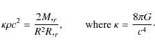
2 The Lemaître-Tolman solution
The L-T model is one of two classes of spherically symmetric
solutions![]() of Einstein's equations where the
gravitational source is dust. In comoving and synchronous coordinates, its line
element reads
of Einstein's equations where the
gravitational source is dust. In comoving and synchronous coordinates, its line
element reads
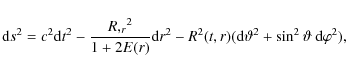
where E(r) is an arbitrary function and
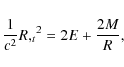
where
The solutions of (2) can be written as
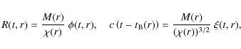
where
- 1.
- when E < 0 (elliptic evolution):
- 2.
- when E = 0 (parabolic evolution):
- 3.
- and when E > 0 (hyperbolic evolution):
Since all the formulae given so far are covariant under coordinate
transformations of the form
![]() ,
one of the functions E(r),
M(r) and
,
one of the functions E(r),
M(r) and
![]() can be fixed at will by the choice of g. Therefore, once
this choice is done, a given L-T model is fully determined by
two of these arbitrary functions.
can be fixed at will by the choice of g. Therefore, once
this choice is done, a given L-T model is fully determined by
two of these arbitrary functions.
However, as shown by Mustapha et al. (1998), and used as an illustration
for application to the supernova data and the ``cosmological constant problem'' by
Célérier (2000), a set of isotropic data corresponding to a given observable
can constrain only one of the two free functions, and therefore the fitting of
the supernova data, i.e. of the function
![]() ,
with a given L-T solution,
still leaves the other function free - and available for fitting to another set
of data. Thus, we must also assume another set of initial conditions, e.g. the
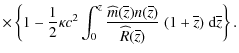
redshift-space mass-density m(z) n(z) or the expansion rate H(z). We will
take these functions to be identical to the corresponding functions in the
,
with a given L-T solution,
still leaves the other function free - and available for fitting to another set
of data. Thus, we must also assume another set of initial conditions, e.g. the
redshift-space mass-density m(z) n(z) or the expansion rate H(z). We will
take these functions to be identical to the corresponding functions in the
![]() CDM model, assuming they reflect the observational data. By this, we
want to show that there is no antagonism between the inhomogeneous cosmology and
the
CDM model, assuming they reflect the observational data. By this, we
want to show that there is no antagonism between the inhomogeneous cosmology and
the ![]() CDM model, and that the first can predict the same results as the
second even if
CDM model, and that the first can predict the same results as the
second even if ![]() .
However, whenever possible we present the real data
to show that there is still much room within observational errors for different
profiles.
.
However, whenever possible we present the real data
to show that there is still much room within observational errors for different
profiles.
Using the reciprocity theorem (Etherington 1933; Ellis 1971) the luminosity
distance can be converted to the angular diameter distance
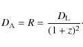
|
(8) |
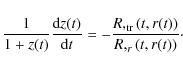
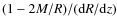
For a ray issued from a radiating source and proceeding towards the central observer on a radial null geodesic the following equation holds
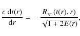
and the equation for the redshift reads (Bondi 1947; Plebanski & Krasinski 2006):
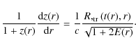
For later reference we will need also the following equation, which follows easily from (9) and (10):
3 The L-T model with no central void
Our aim is now to show we can design an L-T model with no central void able to
reproduce the angular diameter distance-redshift relation as inferred from the
SN Ia data, smoothed out as in the framework of a ![]() CDM model. For this
purpose, we propose to use the following additional conditions to specify the
arbitrary functions M(r), E(r) and
CDM model. For this
purpose, we propose to use the following additional conditions to specify the
arbitrary functions M(r), E(r) and
![]() .
.
3.1 The model defined by D (z) and m(z) n(z)
3.1.1 The MHE procedure
The algorithm used to find the L-T model reproducing the
![]() and n(z)data was first developed by Mustapha et al. (1997). Let us recall its
major steps and equations.
and n(z)data was first developed by Mustapha et al. (1997). Let us recall its
major steps and equations.
The radial coordinate r is chosen so that, on the past light cone of
(t, r) = (t0, 0),

(Note: this choice of r is possible only on a single light cone. In the following, we always refer to the light cone of (t, r) = (t0, 0).) This choice of coordinates simplifies the null geodesic equation:

where we denote quantities on this null cone by a hat. Furthermore, (3) now becomes
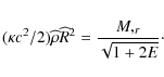
The total derivative of the areal radius R gives
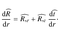
Using (2), (12) and (13), the above equation can be written as
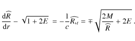
This can be solved for E(r):
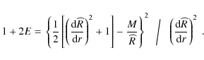
Using (14) the above becomes
![\begin{displaymath}\frac {{\rm d} {M}} {{\rm d} {r}} + \left({\displaystyle{\fra...
... {{\rm d} {\widehat{R}}} {{\rm d} {r}}\right)^2 + 1 \right] .
\end{displaymath}](/articles/aa/full_html/2010/10/aa13581-09/img59.png)
Matter density can be expressed in terms of n(z) - the observed number density of sources in the redshift space per steradian per unit redshift interval. Thus, the number of sources observed in a given redshift interval and solid angle
where
where

Finally, to find r(z), the r.h.s. of (10) must be expressed in terms of
![\begin{displaymath}{\widehat{\frac{R,_{\rm tr}}{\sqrt{1 + 2E} ~}}} =
\frac{c^2}...
... -
\frac{M}{\widehat{R}^2} + ({\sqrt{1 + 2E} ~}),_r \right].
\end{displaymath}](/articles/aa/full_html/2010/10/aa13581-09/img71.png)
|
(22) |
The derivative of
Now, from (10):
|
(24) |
Applying

and integrating with respect to r, yields
| |
![$\displaystyle \left[\frac {{\rm d} {\overline{z}}} {{\rm d} {r}}
\frac {{\rm d} {\widehat{R}}} {{\rm d} {\overline{z}}} (1 + \overline{z}) \right]
{\rm d} r$](/articles/aa/full_html/2010/10/aa13581-09/img77.png)
|
||
|
(25) |
Using the origin conditions
![$\displaystyle \left[ \frac {{\rm d} {\widehat{R}}} {{\rm d} {z}} (1 + z) \right]^{-1}$](/articles/aa/full_html/2010/10/aa13581-09/img81.png)
Finally:
![$\displaystyle \int_0^z \left[ \frac {{\rm d} {\widehat{R}}} {{\rm d} {\tilde{z}}} (1 + \tilde{z})
\right]$](/articles/aa/full_html/2010/10/aa13581-09/img83.png)
![\begin{figure}
\par\includegraphics[width=7.5cm,clip]{13581fg2.eps}
\end{figure}](/articles/aa/full_html/2010/10/aa13581-09/img85.png)
|
Figure 2:
The function E(r) of the L-T model defined by the
|
| Open with DEXTER | |
3.1.2 The algorithm
In order to specify the model, we proceed in the following way:
- 1.
- The model is defined by two functions on the
past null cone: the angular diameter distance,
 ,
and the mass density in
redshift space, m(z)n(z). We assume that these functions are the same as in
the
,
and the mass density in
redshift space, m(z)n(z). We assume that these functions are the same as in
the  CDM model:
where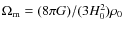 .
.
- 2.
- Using the MHE algorithm we find r(z) by solving (27).
- 3.
- We numerically invert this relation to find z(r) and solve (18) to find M(r).
- 4.
- The function E(r) is found by solving (17).
- 5.
- Once E and M are known, we find
 and then
  ,
by solving the appropriate relations (4)-(7).
,
by solving the appropriate relations (4)-(7).
- 6.
- Since in (17) the term
 becomes 0/0 at the
apparent horizon, the computer produces inaccurate results in the vicinity. To
overcome this we apply the procedure described in Sect. 3.1.4.
becomes 0/0 at the
apparent horizon, the computer produces inaccurate results in the vicinity. To
overcome this we apply the procedure described in Sect. 3.1.4.
3.1.3 The results
The algorithm described in the previous section allows us to find an L-T model
from a given
![]() set of data.
set of data.
The free functions of the L-T model, E, ![]() ,
and M are shown in Figs. 2, 3, and 4 respectively.
,
and M are shown in Figs. 2, 3, and 4 respectively.
As can be seen, there is a problem with numerical integration for E and ![]() around r=2.9 Gpc. The problem is related to (17) where the term
around r=2.9 Gpc. The problem is related to (17) where the term
![]() becomes 0/0 at the apparent horizon. Because of this, the
computer produces inaccurate results in the vicinity. One solution to this
problem was proposed by Lu & Hellaby (2007) who performed series expansions of
R(z), n(z),
becomes 0/0 at the apparent horizon. Because of this, the
computer produces inaccurate results in the vicinity. One solution to this
problem was proposed by Lu & Hellaby (2007) who performed series expansions of
R(z), n(z),
![]() ,
M(z) and E(z) around the apparent horizon.
However, this method leads either to jumps in one of these functions, say
E(z), or to lower accuracy of the algorithm (Lu & Hellaby 2007). Therefore,
we propose a different, much simpler approach. Namely, we fit polynomials to
E(r) and M(r) and then we recalculate the area distance and the
redshift-space mass-density as functions of redshift to check the accuracy of
our approximations. As we will see, this method leads to results that from the
observational point of view (every observation is accompanied with an error) are
indistinguishable from those of the
,
M(z) and E(z) around the apparent horizon.
However, this method leads either to jumps in one of these functions, say
E(z), or to lower accuracy of the algorithm (Lu & Hellaby 2007). Therefore,
we propose a different, much simpler approach. Namely, we fit polynomials to
E(r) and M(r) and then we recalculate the area distance and the
redshift-space mass-density as functions of redshift to check the accuracy of
our approximations. As we will see, this method leads to results that from the
observational point of view (every observation is accompanied with an error) are
indistinguishable from those of the ![]() CDM model.
CDM model.
![\begin{figure}
\par\includegraphics[width=7.5cm,clip]{13581fg3.eps}
\end{figure}](/articles/aa/full_html/2010/10/aa13581-09/img91.png)
|
Figure 3:
The function
|
| Open with DEXTER | |
![\begin{figure}
\par\includegraphics[width=7.5cm,clip]{13581fg4.eps}
\end{figure}](/articles/aa/full_html/2010/10/aa13581-09/img92.png)
|
Figure 4:
The function M(r) of the L-T model defined by the
|
| Open with DEXTER | |
![\begin{figure}
\par\includegraphics[width=7.5cm,clip]{13581fg5.eps}
\end{figure}](/articles/aa/full_html/2010/10/aa13581-09/img93.png)
|
Figure 5:
The function E as a function of the current areal radius for the
|
| Open with DEXTER | |
3.1.4 Dealing with the apparent horizon
To overcome the numerical problem of indeterminacy of E(r) at the apparent
horizon, we fit polynomials to the obtained M(r) and E(r). The most obvious
choice would be polynomials in the variable r. However, in numerical
experiments we noticed that much better results are obtained when we approximate
M and E by polynomials in R(t0, r), where t0 is the present instant.
The explicit forms of the fitted functions are
where
where
![\begin{figure}
\par\includegraphics[width=7.5cm,clip]{fig6r.eps}
\end{figure}](/articles/aa/full_html/2010/10/aa13581-09/img107.png)
|
Figure 6:
The function M as a function of the current areal radius for the
|
| Open with DEXTER | |
The profiles of these functions together with those numerically derived are
presented in Figs. 5 and 6. We then use these functions as
initial conditions and solve the null geodesic equations. First, we invert (10) and (11) to get the equations for
![]() and
and
![]() ,
to derive the pair (t,r) for a given redshift;
simultaneously we solve (2) to get
,
to derive the pair (t,r) for a given redshift;
simultaneously we solve (2) to get
![]() ,
,
![]() ,
and
,
and
![]() .
.
The results are shown in Figs. 7, 8. The angular diameter
distance is recovered very accurately, while the redshift-space mass-density
less so, but still up to z=4 it does not differ by more than ![]() from the
redshift-space mass-density in the
from the
redshift-space mass-density in the ![]() CDM model - which is far less than
the expected observational uncertainty. In addition we calculate the prediction
for H(z), and we compare it to the estimations of the expansion rate by Simon
et al. (2005). Since these are based on the observed age of the oldest
stars, and H(z) follows from
CDM model - which is far less than
the expected observational uncertainty. In addition we calculate the prediction
for H(z), and we compare it to the estimations of the expansion rate by Simon
et al. (2005). Since these are based on the observed age of the oldest
stars, and H(z) follows from
![]() ,
thus, as seen from (11),
,
thus, as seen from (11),
![]() .
The results are presented in Fig. 9. As seen, the L-T model does not deviate from the
.
The results are presented in Fig. 9. As seen, the L-T model does not deviate from the ![]() CDM
model by more than
CDM
model by more than ![]() .
These differences in m(z) n(z) and H(z) are caused
by two factors: a) the Eqs. (30) and (31) are just
approximations; b) numerical errors in the vicinity of the apparent horizon bias
the solution of (17) for
.
These differences in m(z) n(z) and H(z) are caused
by two factors: a) the Eqs. (30) and (31) are just
approximations; b) numerical errors in the vicinity of the apparent horizon bias
the solution of (17) for
![]() (where
(where
![]() is the
position of the apparent horizon). In principle, however, it is possible to
construct the
is the
position of the apparent horizon). In principle, however, it is possible to
construct the ![]() L-T model that matches the
L-T model that matches the ![]() CDM model.
Finally, as seen from Fig. 10,
the current density profile does not
exhibit a giant void shape. Instead, it suggests that the universe
smoothed out
around us with respect to directions is overdense in our vicinity up to
Gpc-scales. As a consequence of our numerical procedure the value of
density at the centre at the present time t0 is the same as the present density in the
CDM model.
Finally, as seen from Fig. 10,
the current density profile does not
exhibit a giant void shape. Instead, it suggests that the universe
smoothed out
around us with respect to directions is overdense in our vicinity up to
Gpc-scales. As a consequence of our numerical procedure the value of
density at the centre at the present time t0 is the same as the present density in the ![]() CDM model.
CDM model.
![\begin{figure}
\par\includegraphics[width=7.5cm,clip]{13581fg7.eps}\vspace{2mm}
\end{figure}](/articles/aa/full_html/2010/10/aa13581-09/img114.png)
|
Figure 7:
The angular diameter distance as a function of redshift; comparison of
the results for the |
| Open with DEXTER | |
![\begin{figure}
\par\includegraphics[width=7.5cm,clip]{13581fg8.eps}\vspace{2mm}
\end{figure}](/articles/aa/full_html/2010/10/aa13581-09/img115.png)
|
Figure 8:
The redshift-space mass-density as a function of redshift.
The difference between the LT and |
| Open with DEXTER | |
![\begin{figure}
\par\includegraphics[width=7.5cm,clip]{13581fg9.eps}
\end{figure}](/articles/aa/full_html/2010/10/aa13581-09/img116.png)
|
Figure 9:
The function H(z). See Sect. 3.1.4 for details. For comparison
the measurements of H(z) (Simon et al. 2005) are also shown. The
difference between the LT and |
| Open with DEXTER | |
![\begin{figure}
\par\includegraphics[width=7.5cm,clip]{13581fg10.eps}
\end{figure}](/articles/aa/full_html/2010/10/aa13581-09/img117.png)
|
Figure 10:
The ratio
|
| Open with DEXTER | |
3.2 The model defined by D (z) and H(z)
3.2.1 The algorithm
The algorithm used to find the L-T model consists of the following steps:
- 1.
- The model is defined by two functions on the
past null cone: the angular diameter distance
and the Hubble function
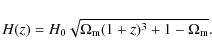
H(z). We assume that these functions are the same as in the CDM
model -
is given by (28) and
- 2.
- We choose r so that (12) is satisfied
on the past light cone of the present-day observer. Then using
 , (10) becomes
(33)
which for (32) can be integrated to
r = 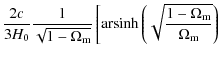
![$\displaystyle \left. -
{\rm arsinh} \left( \sqrt{ \frac{1-\Omega_{\rm m}}{\Omega_{\rm m} (1+z)^3}} \right) \right].$](/articles/aa/full_html/2010/10/aa13581-09/img121.png)
(34)
- 3.
- Using (23) we find
 and solve (21) for
n(z).
and solve (21) for
n(z).
- 4.
- We solve (18) to find M(r).
- 5.
- The function E(r) is found by solving (17).
- 6.
- Once E and M are known we find
and then by solving the appropriate relations (4)-(7).
- 7.
- As before, because of the 0/0 term in (17) at the apparent horizon, we employ the procedure described in Sect. 3.2.3.
3.2.2 The results
The results for E, ![]() and M are given in Figs. 11-13.
As in Sect. 3.1.3, the functions E(r) and
and M are given in Figs. 11-13.
As in Sect. 3.1.3, the functions E(r) and
![]() evaluated by this
algorithm behave unnaturally close to the apparent horizon, see Figs. 11
and 12. As before, this is caused by the fact that in (17) one
has to deal with 0/0. We overcome this problem by once again fitting polynomials
to these functions.
evaluated by this
algorithm behave unnaturally close to the apparent horizon, see Figs. 11
and 12. As before, this is caused by the fact that in (17) one
has to deal with 0/0. We overcome this problem by once again fitting polynomials
to these functions.
![\begin{figure}
\par\includegraphics[width=7.5cm,clip]{13581fg11.eps}
\end{figure}](/articles/aa/full_html/2010/10/aa13581-09/img123.png)
|
Figure 11:
The function E(r) of the L-T model defined by the
|
| Open with DEXTER | |
![\begin{figure}
\par\includegraphics[width=7.5cm,clip]{13581fg12.eps}
\end{figure}](/articles/aa/full_html/2010/10/aa13581-09/img124.png)
|
Figure 12:
The function
|
| Open with DEXTER | |
![\begin{figure}
\par\includegraphics[width=7.6cm,clip]{fig13r.eps}
\end{figure}](/articles/aa/full_html/2010/10/aa13581-09/img125.png)
|
Figure 13:
The function M(r) of the L-T model defined by the
|
| Open with DEXTER | |
![\begin{figure}
\par\includegraphics[width=7.5cm,clip]{13581fg14.eps}
\end{figure}](/articles/aa/full_html/2010/10/aa13581-09/img126.png)
|
Figure 14:
The function E as a function of the current areal radius for the
|
| Open with DEXTER | |
![\begin{figure}
\par\includegraphics[width=7.5cm,clip]{fig15r.eps}
\end{figure}](/articles/aa/full_html/2010/10/aa13581-09/img127.png)
|
Figure 15:
The function M as a function of the current areal radius for the
|
| Open with DEXTER | |
3.2.3 Dealing with the apparent horizon
The explicit forms of the fitted functions are:

where
where
The profiles of these functions together with the numerically derived ones are
shown in Figs. 14 and 15. We then use these functions as
initial conditions and solve the null geodesic equations. The results are
presented in Figs. 16 and 17. Both the angular diameter
distance and the expansion rate as functions of the redshift are recovered very
accurately. From the observational perspective these two models are
indistinguishable. In addition we present the m(z)n(z) plot. As seen from Fig. 18, it also gives quite an accurate fit, with a deviation from the
![]() CDM model being less than
CDM model being less than ![]() .
Finally, as seen from Fig. 19, the current density profile has a similar shape as in Sect. 3.1.4, and this is not a giant void.
.
Finally, as seen from Fig. 19, the current density profile has a similar shape as in Sect. 3.1.4, and this is not a giant void.
![\begin{figure}
\par\includegraphics[width=7.5cm,clip]{13581fg16.eps}
\end{figure}](/articles/aa/full_html/2010/10/aa13581-09/img134.png)
|
Figure 16: The angular diameter distance as a function of z. See Sect. 3.2.3 for details. |
| Open with DEXTER | |
![\begin{figure}
\par\includegraphics[width=7.5cm,clip]{13581fg17.eps}
\end{figure}](/articles/aa/full_html/2010/10/aa13581-09/img135.png)
|
Figure 17: The function H(z). See Sect. 3.2.3 for details. For comparison the measurements of H(z) (Simon et al. 2005) are also shown. |
| Open with DEXTER | |
![\begin{figure}
\par\includegraphics[width=7.5cm,clip]{13581fg18.eps}
\end{figure}](/articles/aa/full_html/2010/10/aa13581-09/img136.png)
|
Figure 18:
The redshift-space mass-density as a function of redshift for the LT
model considered in Sect. 3.2.3, and in the |
| Open with DEXTER | |
![\begin{figure}
\par\includegraphics[width=7.5cm,clip]{13581fg19.eps}
\end{figure}](/articles/aa/full_html/2010/10/aa13581-09/img137.png)
|
Figure 19:
The ratio
|
| Open with DEXTER | |
4 Discussion and conclusion
Contrary to what is commonly claimed, L-T models with a giant void do not
reproduce the main features of the ![]() CDM model. These types of models
just fit cosmological observations, with a priori constraints imposed on the
L-T models. Indeed, we have found the L-T models that mimic some of the
observational features of the
CDM model. These types of models
just fit cosmological observations, with a priori constraints imposed on the
L-T models. Indeed, we have found the L-T models that mimic some of the
observational features of the ![]() CDM model and exhibit no giant void, but
rather a giant hump.
CDM model and exhibit no giant void, but
rather a giant hump.
It is clear from the energy density profiles shown in Figs. 10 and 19
that the L-T models we have reconstructed have a large overdensity,
when viewed over large enough scales. However, as we have made clear
throughout, these profiles are the result of reproducing observables
that match ![]() CDM
predictions, and not from fitting to any real data. Luminosity
distances from supernovae observations, and number counts from galaxy
surveys do not currently extend much beyond
CDM
predictions, and not from fitting to any real data. Luminosity
distances from supernovae observations, and number counts from galaxy
surveys do not currently extend much beyond
![]() and
and
![]() ,
respectively. As such, using real observables, it would only currently
be possible to perform a reconstruction of a limited part of the full
structure we have found here, and even then only up to the degree
allowed by the errors associated with these quantities. If one were to
attempt such a reconstruction, it appears from Figs. 10 and 19 that one may, in fact, reconstruct a local energy density profile that is an increasing function of r, and not decreasing, due to the limited extent of these observations in z
(this is particularly true in the equal age foliation). Our
interpretation of a giant hump should therefore be understood as
corresponding to an extrapolation of observable quantities under the
expectation that they will follow
,
respectively. As such, using real observables, it would only currently
be possible to perform a reconstruction of a limited part of the full
structure we have found here, and even then only up to the degree
allowed by the errors associated with these quantities. If one were to
attempt such a reconstruction, it appears from Figs. 10 and 19 that one may, in fact, reconstruct a local energy density profile that is an increasing function of r, and not decreasing, due to the limited extent of these observations in z
(this is particularly true in the equal age foliation). Our
interpretation of a giant hump should therefore be understood as
corresponding to an extrapolation of observable quantities under the
expectation that they will follow ![]() CDM, rather than being directly implied by any currently known observations themselves.
CDM, rather than being directly implied by any currently known observations themselves.
Recently, some astrophysicists have begun to take seriously the cosmological
implications of the L-T model. This model, although still simple![]() , is quite powerful and exhibits some features of
general relativistic dynamics, like arbitrary functions in the initial data.
, is quite powerful and exhibits some features of
general relativistic dynamics, like arbitrary functions in the initial data.
As we said earlier in this paper, the belief that an L-T model fitted to
supernova Ia observations necessarily implies the existence of a giant void with
us at the centre was created by arbitrarily limiting the generality of the model. With its free functions fitted to ![]() CDM
features rather than to expectations, the giant void does not
necessarily follow. Rather, one alternative is that the graph of the
density smoothed out over angles around us has the shape of a shallow
and wide valley on top of a giant hump.
CDM
features rather than to expectations, the giant void does not
necessarily follow. Rather, one alternative is that the graph of the
density smoothed out over angles around us has the shape of a shallow
and wide valley on top of a giant hump.
This giant hump may be a feature of the particular L-T model that we ended up
with. Variations in the ![]() CDM parameters would modify the details, and
the observational constraints we considered are not very tight. Future
calculations with other constraints may favor a still different profile at t =
now. Hence we do not wish our paper to become a starting point of a new paradigm
in observational cosmology, aimed at detecting the hump. Before this happens, we
must decide at the theoretical level whether the hump is a necessary
implication of L-T models properly fitted to other observations.
CDM parameters would modify the details, and
the observational constraints we considered are not very tight. Future
calculations with other constraints may favor a still different profile at t =
now. Hence we do not wish our paper to become a starting point of a new paradigm
in observational cosmology, aimed at detecting the hump. Before this happens, we
must decide at the theoretical level whether the hump is a necessary
implication of L-T models properly fitted to other observations.
It must be stressed that this hump is not directly observable. It exists
in the space t = now, of events simultaneous with our present instant in the
cosmological synchronisation, i.e. it is in a space-like relation to us. This is
also the case of the giant void (see, e.g., Fig. 4 of Alnes et al. 2006;
Fig. 1 of García-Bellido & Haugbølle 2008a; Figs. 4 and 6 of Yoo et al. 2008). However, an observational test of the giant void is easier to
complete. The reason is that the models considered in this paper have a
redshift-space mass-density almost the same as in the ![]() CDM model (see
Figs. 8 and 18) and as can be seen from Fig. 20, their
CDM model (see
Figs. 8 and 18) and as can be seen from Fig. 20, their
![]() scales with the redshift in almost the same manner as in the FLRW
model, i.e.
scales with the redshift in almost the same manner as in the FLRW
model, i.e. ![]() (1+z)3. This is not the case of the giant void
(1+z)3. This is not the case of the giant void![]() which does not reproduce these features on the past light
cone (see Figs. 1 and 20). Thus, unlike the giant void, the giant
hump is not observable in
which does not reproduce these features on the past light
cone (see Figs. 1 and 20). Thus, unlike the giant void, the giant
hump is not observable in ![]() or in the number count data.
or in the number count data.
![\begin{figure}
\par\includegraphics[width=7.5cm,clip]{13581fg20.eps}
\end{figure}](/articles/aa/full_html/2010/10/aa13581-09/img141.png)
|
Figure 20:
The density distribution as a function of redshift for the giant
void (GV) L-T model, for the models of Sect. 3.1.4 and 3.2.3
(GH) and for the FLRW model, where
|
| Open with DEXTER | |
What is the cause of this difference between the density distribution on our past light cone and in the t = now space? It is the oft-forgotten basic feature of the L-T model (and in fact of all inhomogeneous models, also those not yet known explicitly as solutions of Einstein's equations): on any initial data hypersurface, whether it is a light cone or a t = constant space, the density and velocity distributions are two algebraically independent functions of position. Thus the density on a later hypersurface may be quite different, since it depends on both initial functions. Whatever initial density distribution we observe can be completely transformed by the velocity distribution. For example, as predicted by Mustapha & Hellaby (2001) and explicitly demonstrated by Krasinski & Hellaby (2004), any initial condensation can evolve into a void and vice versa. In FLRW models, there are no physical functions of position, and all worldlines evolve together. Thus, while dealing with an L-T (or any inhomogeneous) model, one must be cautious when applying the Robertson-Walker-inspired prejudices and expectations.
The use of oversimplified L-T models can create another false idea and false
expectation. The false idea is that there is an opposition between the
![]() CDM
model, belonging to the FLRW class, and the L-T model or in general,
inhomogeneous models: either one or the other could be ``correct'', but
not both. This putative opposition can then give rise to the
expectation that more, and more detailed, observations will be able to
tell us which one to reject. In truth, there is no opposition. The
inhomogeneous models, like for example the L-T model with its two
arbitrary functions of one variable are huge, compared to
FLRW, families of models that include the Friedmann models as a very
simple subcase. The fact, demonstrated in several papers already (see
Célérier 2007, for a review), that even a
CDM
model, belonging to the FLRW class, and the L-T model or in general,
inhomogeneous models: either one or the other could be ``correct'', but
not both. This putative opposition can then give rise to the
expectation that more, and more detailed, observations will be able to
tell us which one to reject. In truth, there is no opposition. The
inhomogeneous models, like for example the L-T model with its two
arbitrary functions of one variable are huge, compared to
FLRW, families of models that include the Friedmann models as a very
simple subcase. The fact, demonstrated in several papers already (see
Célérier 2007, for a review), that even a
![]() L-T model can
imitate
L-T model can
imitate
![]() in an FLRW model, additionally attests to the
flexibility and power of the L-T model. Thus, if the Friedmann models,
in an FLRW model, additionally attests to the
flexibility and power of the L-T model. Thus, if the Friedmann models,
![]() CDM among them, are considered good enough for cosmology, then the L-T
models can only be better: they constitute an exact perturbation of the
Friedmann background, and can reproduce the latter as a limit with an arbitrary
precision. While future observations, for example the kSZ effect
(Garcia-Bellido & Haugbølle 2008b) or the growth of linear structure (Clarkson et al. 2009)
will provide a sufficient insight to test particular configurations
(like for example a giant void model), we will never be able to reject
inhomogeneous models. After all, the Universe as it is, is
inhomogeneous. Nowadays we use homogeneous models just for simplicity,
and although they have worked well so far, in future they will
certainly be replaced by more sophisticated models, either by exact
solutions, or what is more probable in light of increasing computation
power of computers, by numerical simulations.
CDM among them, are considered good enough for cosmology, then the L-T
models can only be better: they constitute an exact perturbation of the
Friedmann background, and can reproduce the latter as a limit with an arbitrary
precision. While future observations, for example the kSZ effect
(Garcia-Bellido & Haugbølle 2008b) or the growth of linear structure (Clarkson et al. 2009)
will provide a sufficient insight to test particular configurations
(like for example a giant void model), we will never be able to reject
inhomogeneous models. After all, the Universe as it is, is
inhomogeneous. Nowadays we use homogeneous models just for simplicity,
and although they have worked well so far, in future they will
certainly be replaced by more sophisticated models, either by exact
solutions, or what is more probable in light of increasing computation
power of computers, by numerical simulations.
When considering models that go beyond the FLRW approximation,
one may ask either ``what limitations on the arbitrary functions in the
models do our observations impose'', or ``which model best describes a
given situation: a homogeneous FLRW model or an inhomogeneous one?''
The latter of these questions has often been asked in the context of
comparing L-T models without ![]() to FLRW models with
to FLRW models with ![]() ,
and is of much interest for understanding the necessity of introducing
,
and is of much interest for understanding the necessity of introducing ![]() into the observer's standard cosmological model. Such hypothesis
testing questions are often posed in cosmology, but are difficult to
address in the current context as they require artificially limiting
the generality of the models in question (in order to have a finite
number of parameters, so that the test can be performed). Given the
lack of motivation for exactly how to perform such a limitation, one is
then left in the undesirable circumstance of (potentially) dismissing
particular L-T models, while being left with an infinite number of
remaining L-T models to evaluate. We therefore prefer to consider the
former question. In order to reasonably answer this for the L-T model,
a general framework for interpreting observations in the L-T
geometrical
background should be created (and in the future it should be
transformed into a
framework for interpreting the observations in a still more general, or
the
most general geometrical background). Such a program is still in its infancy,
but is being actually developed by C. Hellaby and coworkers under the name
``Metric of the Cosmos'' (Lu & Hellaby 2007; McClure & Hellaby 2008; Hellaby & Alfedeel 2009).
into the observer's standard cosmological model. Such hypothesis
testing questions are often posed in cosmology, but are difficult to
address in the current context as they require artificially limiting
the generality of the models in question (in order to have a finite
number of parameters, so that the test can be performed). Given the
lack of motivation for exactly how to perform such a limitation, one is
then left in the undesirable circumstance of (potentially) dismissing
particular L-T models, while being left with an infinite number of
remaining L-T models to evaluate. We therefore prefer to consider the
former question. In order to reasonably answer this for the L-T model,
a general framework for interpreting observations in the L-T
geometrical
background should be created (and in the future it should be
transformed into a
framework for interpreting the observations in a still more general, or
the
most general geometrical background). Such a program is still in its infancy,
but is being actually developed by C. Hellaby and coworkers under the name
``Metric of the Cosmos'' (Lu & Hellaby 2007; McClure & Hellaby 2008; Hellaby & Alfedeel 2009).
M.N.C. wants to acknowledge interesting discussions with Rocky Kolb, Luca Amendola, Roberto Sussman and Miguel Quartin. We also acknowledge useful comments on earlier versions of this text by Charles Hellaby. The work of AK was partly supported by the Polish Ministry of Higher Education grant N202 104 838.
References
- Alexander, S., Biswas, T., Notari, A., & Vaid, D. 2009, JCAP, 0909, 025 [NASA ADS] [CrossRef] [Google Scholar]
- Alnes, H., & Amarzguioui, M. 2007, Phys. Rev. D, 75, 023506 [NASA ADS] [CrossRef] [Google Scholar]
- Alnes, H., Amarzguioui, M., & Grøn, Ø. 2006, Phys. Rev. D, 73, 083519 [NASA ADS] [CrossRef] [Google Scholar]
- Apostolopoulos, P. S., Brouzakis, N., Tetradis, N., et al. 2006, JCAP, 0606, 009 [NASA ADS] [Google Scholar]
- Biswas, T., & Notari, A. 2008, JCAP, 0806, 021 [NASA ADS] [CrossRef] [Google Scholar]
- Bolejko, K. 2008, PMC Phys. A, 2, 1 [Google Scholar]
- Bolejko, K. 2009, GRG, 41, 1737 [Google Scholar]
- Bolejko, K., & Wyithe, J. S. B. 2009, JCAP, 0902, 020 [Google Scholar]
- Bolejko, K., Krasinski, A., & Hellaby, C. 2005, MNRAS, 362, 213 [NASA ADS] [CrossRef] [Google Scholar]
- Bondi, H. 1947, MNRAS, 107, 410 [NASA ADS] [CrossRef] [Google Scholar]
- Brouzakis, N., Tetradis, N., & Tzavara, E. 2007, JCAP, 0702, 013 [NASA ADS] [CrossRef] [Google Scholar]
- Buchert, T. 2000, GRG, 32, 105 [Google Scholar]
- Buchert, T. 2001, GRG, 33, 1381 [Google Scholar]
- Célérier, M. N. 2000, A&A 353, 63. [Google Scholar]
- Célérier, M. N. 2007, New Adv. Phys., 1, 29 [Google Scholar]
- Clarkson, C., Clifton, T., & February, S. 2009, JCAP, 0906, 025 [Google Scholar]
- Clifton, T., Ferreira, P. G., & Zuntz, J. 2009, JCAP, 0907, 029 [Google Scholar]
- Ellis, G. F. R. 1971, Proceedings of the International School of Physics Enrico Fermi, Course 47: General Relativity and Cosmology, ed. R. K. Sachs (New York and London: Academic Press), 104; reprinted, with historical comments, in 2009, GRG, 41, 581 [Google Scholar]
- Enqvist, K., & Mattsson, T. 2007, JCAP, 0702, 019 [Google Scholar]
- Etherington, I. M. H. 1933, Phil. Mag. VII, 15, 761 [Google Scholar]
- ; reprinted, with historical comments, in 2007, GRG, 39, 1055 [Google Scholar]
- García-Bellido, J., & Haugbølle, T. 2008a, JCAP, 0804, 003 [Google Scholar]
- García-Bellido, J., & Haugbølle, T. 2008b, JCAP, 0809, 016 [Google Scholar]
- García-Bellido, J., & Haugbølle, T. 2009, JCAP, 0909, 028 [NASA ADS] [Google Scholar]
- Hellaby, C., & Alfedeel, A. H. A. 2009, Phys. Rev. D, 79, 043501 [NASA ADS] [CrossRef] [Google Scholar]
- Iguchi, H., Nakamura, T., & Nakao, K. 2002, Prog. Theor. Phys., 108, 809 [NASA ADS] [CrossRef] [Google Scholar]
- Kowalski, M., Rubin, D., Aldering, G., et al. 2008, ApJ, 686, 749 [NASA ADS] [CrossRef] [Google Scholar]
- Krasinski, A., & Hellaby, C. 2004, Phys. Rev. D, 69, 023502 [NASA ADS] [CrossRef] [Google Scholar]
- Lemaître, G. 1933, Ann. Soc. Sci. Bruxelles A53, 51; English translation, with historical comments: 1997, GRG, 29, 637 [Google Scholar]
- Lu, T. H. C., & Hellaby, C. 2007, CQG, 24, 4107 [NASA ADS] [CrossRef] [Google Scholar]
- Marra, V., Kolb, E. W., Matarrese, S., et al. 2007, Phys. Rev. D, 76, 123004 [NASA ADS] [CrossRef] [MathSciNet] [Google Scholar]
- McClure, M. L., & Hellaby, C. 2008, Phys. Rev. D, 78, 044005 [Google Scholar]
- Mustapha, N., & Hellaby, C. 2001, GRG, 33, 455 [Google Scholar]
- Mustapha, N., Hellaby, C., & Ellis, G. F. R. 1997, MNRAS, 292, 817 [NASA ADS] [Google Scholar]
- Mustapha, N., Bassett, B. A. C. C., Hellaby, C., et al. 1998, CQG, 15, 2363 [Google Scholar]
- Pascual-Sánchez, J. F. 1999, Mod. Phys. Lett. A, 14, 1539 [NASA ADS] [CrossRef] [Google Scholar]
- Plebanski, J., & Krasinski, A. 2006, An Introduction to General Relativity and Cosmology (Cambridge University Press) [Google Scholar]
- Ruban, V. A. 1968, Pis'ma v Red. ZhETF, 8, 669 [NASA ADS] [Google Scholar]
- ; English translation: Sov. Phys. JETP Lett., 8, 414 (1968); reprinted, with historical comments: 2001, GRG, 33, 363 [Google Scholar]
- Ruban, V. A. 1969, Zh. Eksper. Teor. Fiz., 56, 1914 [Google Scholar]
- ; English translation: Sov. Phys. JETP, 29, 1027 (1969); reprinted, with historical comments: 2001, GRG, 33, 375 [Google Scholar]
- Silk, J. 1977, A&A, 59, 53 [NASA ADS] [Google Scholar]
- Schneider, J., & Célérier, M. N. 1999, A&A, 348, 25 [NASA ADS] [Google Scholar]
- Simon, J., Verde, L., & Jimenez, R. 2005, Phys. Rev. D, 71, 123001 [Google Scholar]
- Tolman, R. C. 1934, Proc. Nat. Acad. Sci. USA, 20, 169 [NASA ADS] [CrossRef] [Google Scholar]
- ; reprinted, with historical comments: 1997, GRG, 29, 931 [Google Scholar]
- Yoo, C. M., Kai, T., & Nakao, K.-I. 2008, Prog. Theor. Phys., 120, 937 [NASA ADS] [CrossRef] [Google Scholar]
- Zibin, J. P., Moss, A., & Scott, D. 2008, Phys. Rev. Lett., 101, 251303 [NASA ADS] [CrossRef] [PubMed] [Google Scholar]
Footnotes
- ...2007)
![[*]](/icons/foot_motif.png)
- However, these authors have shown that the CMB data put very stringent limits on the distance of the observer from the centre of the model or/and on the amplitude of the inhomogeneities in an off-centre observer model.
- ...
observations
- One should be aware that there is a great deal of
phenomenology involved in interpreting the observations. For example, with
supernovae, the cosmological model predicts
 ,
while what is actually
observed is the flux. We can deduce the absolute luminosity only on the basis of
some empirical methods. Similarly with galaxy number counts - the cosmological
model predicts m(z) n(z) where m(z) is an average mass per source and n(z)is number counts. The whole information about the galaxy evolution and their
mergers is encoded in m(z) - however in galaxy redshift surveys we observe
only n(z). In this paper we do not focus on the problem of observations and
assume
and mn as in the CDM.
,
while what is actually
observed is the flux. We can deduce the absolute luminosity only on the basis of
some empirical methods. Similarly with galaxy number counts - the cosmological
model predicts m(z) n(z) where m(z) is an average mass per source and n(z)is number counts. The whole information about the galaxy evolution and their
mergers is encoded in m(z) - however in galaxy redshift surveys we observe
only n(z). In this paper we do not focus on the problem of observations and
assume
and mn as in the CDM.
- ...
solutions
- For the presentation of the other class see Plebanski & Krasinski (2006). It is called there the Datt-Ruban solution (Ruban 1968, 1969). It has interesting geometrical and physical properties, but so far has found no astrophysical application.
- ... simple
- From the computational point of view, the difference between the Friedmann and L-T models is quite trivial. The Eq. (2) that governs the evolution of the L-T model is exactly the same as in the Friedmann model; it is still an ordinary differential equation in the time-variable t. The only difference is that the function R(t) obeying (2) depends on one more variable, the radial coordinate r. This r enters only as a parameter, and then automatically all the integration ``constants'' that appear while solving (2) are no longer constant, but are functions of r. Sophistication comes at the level of interpreting the solutions - however, this is no longer mathematics, but astrophysics.
- ... void
- The giant void used here is Bolejko & Wyithe (2009)'s model with radius of 2.96 Gpc and density contrast of 4.05. The redshift-space mass-density for this model is presented in Fig. 1.
All Figures
|
|
Figure 1:
The redshift-space mass-density in the |
| Open with DEXTER | |
| In the text | |
|
|
Figure 2:
The function E(r) of the L-T model defined by the
|
| Open with DEXTER | |
| In the text | |
|
|
Figure 3:
The function
|
| Open with DEXTER | |
| In the text | |
|
|
Figure 4:
The function M(r) of the L-T model defined by the
|
| Open with DEXTER | |
| In the text | |
|
|
Figure 5:
The function E as a function of the current areal radius for the
|
| Open with DEXTER | |
| In the text | |
|
|
Figure 6:
The function M as a function of the current areal radius for the
|
| Open with DEXTER | |
| In the text | |
|
|
Figure 7:
The angular diameter distance as a function of redshift; comparison of
the results for the |
| Open with DEXTER | |
| In the text | |
|
|
Figure 8:
The redshift-space mass-density as a function of redshift.
The difference between the LT and |
| Open with DEXTER | |
| In the text | |
|
|
Figure 9:
The function H(z). See Sect. 3.1.4 for details. For comparison
the measurements of H(z) (Simon et al. 2005) are also shown. The
difference between the LT and |
| Open with DEXTER | |
| In the text | |
|
|
Figure 10:
The ratio
|
| Open with DEXTER | |
| In the text | |
|
|
Figure 11:
The function E(r) of the L-T model defined by the
|
| Open with DEXTER | |
| In the text | |
|
|
Figure 12:
The function
|
| Open with DEXTER | |
| In the text | |
|
|
Figure 13:
The function M(r) of the L-T model defined by the
|
| Open with DEXTER | |
| In the text | |
|
|
Figure 14:
The function E as a function of the current areal radius for the
|
| Open with DEXTER | |
| In the text | |
|
|
Figure 15:
The function M as a function of the current areal radius for the
|
| Open with DEXTER | |
| In the text | |
|
|
Figure 16: The angular diameter distance as a function of z. See Sect. 3.2.3 for details. |
| Open with DEXTER | |
| In the text | |
|
|
Figure 17: The function H(z). See Sect. 3.2.3 for details. For comparison the measurements of H(z) (Simon et al. 2005) are also shown. |
| Open with DEXTER | |
| In the text | |
|
|
Figure 18:
The redshift-space mass-density as a function of redshift for the LT
model considered in Sect. 3.2.3, and in the |
| Open with DEXTER | |
| In the text | |
|
|
Figure 19:
The ratio
|
| Open with DEXTER | |
| In the text | |
|
|
Figure 20:
The density distribution as a function of redshift for the giant
void (GV) L-T model, for the models of Sect. 3.1.4 and 3.2.3
(GH) and for the FLRW model, where
|
| Open with DEXTER | |
| In the text | |
Copyright ESO 2010
Current usage metrics show cumulative count of Article Views (full-text article views including HTML views, PDF and ePub downloads, according to the available data) and Abstracts Views on Vision4Press platform.
Data correspond to usage on the plateform after 2015. The current usage metrics is available 48-96 hours after online publication and is updated daily on week days.
Initial download of the metrics may take a while.