| Issue |
A&A
Volume 517, July 2010
|
|
|---|---|---|
| Article Number | L4 | |
| Number of page(s) | 4 | |
| Section | Letters | |
| DOI | https://doi.org/10.1051/0004-6361/201015169 | |
| Published online | 30 July 2010 | |
LETTER TO THE EDITOR
Lepton models for TeV emission from SNR RX J1713.7-3946
Z. H. Fan1 - S. A. Liu2 - Q. Yuan3 - L. Fletcher2
1 - Department of Physics, Yunnan University, Kunming 650091, Yunnan, PR China
2 - Department of Physics and Astronomy, University of Glasgow, Glasgow G12 8QQ, UK
3 - Key Laboratory of Particle Astrophysics, Institute of High
Energy Physics, Chinese Academy of Sciences, Beijing 100049,
PR China
Received 8 June 2010 / Accepted 4 July 2010
Abstract
Aims. SNR RX J1713.7-3946 is perhaps one of the best
observed shell-type supernova remnants with emissions dominated by
energetic particles accelerated near the shock front. The nature of the
TeV emission, however, is an issue still open to investigation.
Methods. We carried out a systematic study of four lepton models for the TeV emission with the Markov chain Monte Carlo method.
Results. It is shown that current data already give good
constraints on the model parameters. Two commonly used parametric
models do not appear to fit the observed radio, X-ray, and ![]() -ray
spectra. Models motivated by diffusive shock acceleration and by
stochastic acceleration by compressive waves in the shock downstream
give comparably good fits. The former has a sharper spectral cutoff in
the hard X-ray band than the latter. Future observations with the HXMT and NuSTAR may distinguish these two models.
-ray
spectra. Models motivated by diffusive shock acceleration and by
stochastic acceleration by compressive waves in the shock downstream
give comparably good fits. The former has a sharper spectral cutoff in
the hard X-ray band than the latter. Future observations with the HXMT and NuSTAR may distinguish these two models.
Key words: acceleration of particles - plasmas - shock waves - turbulence
1 Introduction
Energetic particles produce radiations over a broad energy range under typical astrophysical circumstances. To study the energetic particle population in high-energy astrophysical sources, observations over a broad spectral range are needed. Multi-wavelength observations of individual sources usually give sparse spectral data points, which can be fitted reasonably well with a simple power-law or broken power-law function. A featureless power-law distribution implies the lack of characteristic scales or distinct processes in the system. The nature of particle acceleration processes are still a matter of debate nearly a century after the discovery of high-energy particles from the outer space (Butt 2009).
Recent progress in observations of high-energy astrophysical
sources has resulted in more detailed spectral coverage, and
spectral features start to emerge. These features are produced by
the underlying physical processes with well-defined characteristic
scales in space, time, and/or energy, and they play essential roles in
advancing our understanding of the acceleration mechanism
(Berezhko & Krymsky 1988). Diffusive astrophysical shocks are considered as one of
the most important particle accelerators (Berezhko 1996; Drury 1983; Toptygin 1980). The
acceleration of particles by compressive motions of astrophysical
flows is also a very generic process (Ptuskin 1988). Both processes may
be important in the acceleration of particles dominating the
radiative characteristics of the shock associated with SNR RX J1713.7-394 (Fan et al. 2010). Detailed X-ray and ![]() -ray
observations of this source have revealed several features: 1) the
X-ray and
-ray
observations of this source have revealed several features: 1) the
X-ray and ![]() -ray emissions are well correlated in space
(Plaga 2008; Aharonian et al. 2006); 2) the emission spectrum shows a clear high-energy
cutoff in both the X-ray and TeV bands (Aharonian et al. 2007), and the cutoff in
hard X-rays appears to be sharp (Tanaka et al. 2008), implying a sharp cutoff
in the electron distribution producing the observed radio to X-ray
spectrum through the synchrotron process; 3) the
-ray emissions are well correlated in space
(Plaga 2008; Aharonian et al. 2006); 2) the emission spectrum shows a clear high-energy
cutoff in both the X-ray and TeV bands (Aharonian et al. 2007), and the cutoff in
hard X-rays appears to be sharp (Tanaka et al. 2008), implying a sharp cutoff
in the electron distribution producing the observed radio to X-ray
spectrum through the synchrotron process; 3) the ![]() -ray
spectrum has a broad convex shape (Funk 2009); 4) there are bright
X-ray filaments with a width of
-ray
spectrum has a broad convex shape (Funk 2009); 4) there are bright
X-ray filaments with a width of ![]() 0.1 light year varying on a
timescale of about a year (Uchiyama et al. 2007). Liu et al. (2008) showed that these
emissions may be attributed to a single population of electrons with
the
0.1 light year varying on a
timescale of about a year (Uchiyama et al. 2007). Liu et al. (2008) showed that these
emissions may be attributed to a single population of electrons with
the ![]() -rays produced via the inverse Compton scattering of the
background photons by relativistic electrons.
-rays produced via the inverse Compton scattering of the
background photons by relativistic electrons.
In light of recent high-resolution observations with Suzaku and Fermi, we use the Markov chain Monte Carlo (MCMC) method to constrain parameters of
four possible lepton models. It is shown that simple models with a
power-law electron distribution, which cuts off at TeV energies, give a
poor fit to either the X-ray or ![]() -ray spectrum. Motivated by the
mechanism of diffusive shock acceleration (DSA) and stochastic acceleration
(SA) by compressive motions, we introduce two alternative models, both of
which give acceptable fits to the observed spectra (Sect. 2).
In Sect. 3, we discuss the implications of these results and
future work needed to improve these models. Conclusions are drawn in Sect. 4.
-ray spectrum. Motivated by the
mechanism of diffusive shock acceleration (DSA) and stochastic acceleration
(SA) by compressive motions, we introduce two alternative models, both of
which give acceptable fits to the observed spectra (Sect. 2).
In Sect. 3, we discuss the implications of these results and
future work needed to improve these models. Conclusions are drawn in Sect. 4.
2 Spectral fits with lepton models
In the lepton scenario, the radio to X-ray emissions are produced
through the synchrotron process of relativistic electrons, and the ![]() -ray
emission
is produced through the inverse Compton scattering of the background
radiation
fields by the same electron population. If the background magnetic
fields are relatively uniform, similar to the background radiation
fields, the model can naturally explain the spatial correlation between
the X-rays and
-ray
emission
is produced through the inverse Compton scattering of the background
radiation
fields by the same electron population. If the background magnetic
fields are relatively uniform, similar to the background radiation
fields, the model can naturally explain the spatial correlation between
the X-rays and ![]() -rays
(Plaga 2008). As pointed out by Liu et al. (2008),
the magnetic field required to
produce the X-ray flux agrees with what is required to produce an X-ray
spectral cutoff by an electron population cutting off in the TeV energy
range (Ellision et al. 2010; Aharonian et al. 2007).
-rays
(Plaga 2008). As pointed out by Liu et al. (2008),
the magnetic field required to
produce the X-ray flux agrees with what is required to produce an X-ray
spectral cutoff by an electron population cutting off in the TeV energy
range (Ellision et al. 2010; Aharonian et al. 2007).
There are at least four parameters in a specific model. In this work we employ
an MCMC technique suitable for multi-parameter determination to
search all the model parameters. The
Metropolis-Hastings sampling algorithm is adopted when determining the jump
probability from one point to the next in the parameter space (MacKay 2003).
The MCMC approach, which is based on the Bayesian statistics, is
superior to the grid approach with a more efficient sampling of the
parameter space of interest, especially for high dimensions. The
algorithm ensures that the probability density functions (PDF) of
model parameters can be asymptotically approached with the number
density of samples.
Starting with an initial parameter set ![]() ,
which should
lie in a reasonable parameter space, one obtains the likelihood function of
,
which should
lie in a reasonable parameter space, one obtains the likelihood function of
![]() :
:
![]() .
Then another parameter set
.
Then another parameter set
![]() is randomly selected with the corresponding likelihood function
is randomly selected with the corresponding likelihood function
![]() .
This parameter set is accepted with the probability
.
This parameter set is accepted with the probability
![]() .
If the new point is
accepted, it becomes the starting point for the next step, otherwise, we reset
.
If the new point is
accepted, it becomes the starting point for the next step, otherwise, we reset
![]() .
This procedure is repeated to derive a parameter
chain that determines the PDF of model parameters. More details of this
procedure can be found in Neil (1993), Gamerman (1997), and MacKay (2003).
.
This procedure is repeated to derive a parameter
chain that determines the PDF of model parameters. More details of this
procedure can be found in Neil (1993), Gamerman (1997), and MacKay (2003).
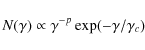
I: Without detailed modeling of the particle acceleration
processes, a power-law electron distribution with an exponential
high-energy cutoff is often assumed to fit the observed spectrum:
|
(1) |
where p is the spectral index,
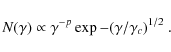
II: Liu et al. (2008) suggested that the fit to the ![]() -ray
spectrum can be improved by considering a more gradual cutoff in
the electron distribution:
-ray
spectrum can be improved by considering a more gradual cutoff in
the electron distribution:
|
(2) |
Several mechanisms can cause variations in the shape of the high-energy cutoff (Blasi 2010; Zirakashvili & Aharonian 2007; Becker et al. 2006; Berezhko & Krymsky 1988). However, given the sharp cutoff of the X-ray spectrum, Tanaka et al. (2008) claim that the electron distribution must have a very steep cutoff. Indeed, by using their data and performing the MCMC fit, we obtain radio fluxes nearly one order of magnitude below the observed values. The model also significantly overestimates the hard X-ray fluxes. To increase the weight of the radio and
III: The particle distribution is determined by the injection
process and the spatial diffusion coefficient ![]() in the DSA model.
The time-dependent electron distribution with a constant injection
rate may be approximated as (Drury 1991; Berezhko & Krymsky 1988; Forman & Drury 1983)
in the DSA model.
The time-dependent electron distribution with a constant injection
rate may be approximated as (Drury 1991; Berezhko & Krymsky 1988; Forman & Drury 1983)
![\begin{displaymath}N(\gamma)\propto \gamma^{-p} \exp
[-9\chi (\gamma)/U^2{T_{\rm life}}]~,
\end{displaymath}](/articles/aa/full_html/2010/09/aa15169-10/img18.png)
where
where e is the elementary charge,
Compared with the previous two models, an extra parameter is introduced
here:
![]() ,
which is proportional to the electron
acceleration timescale. Figures 1 and 2 show the results with
,
which is proportional to the electron
acceleration timescale. Figures 1 and 2 show the results with ![]() .
The probability density of
.
The probability density of
![]() peaks near a typical value of 12. Since
peaks near a typical value of 12. Since ![]() has to be greater than 1, we have
has to be greater than 1, we have
![]() lyr. The gyro-radius of electrons at the
cutoff Lorentz factor
lyr. The gyro-radius of electrons at the
cutoff Lorentz factor
![]() is
is ![]() 0.01 pc
comparable to the width of the observed highly variable X-ray
filaments. The X-ray variability may then be attributed to spatial
diffusion of X-ray emitting electrons from a high-density region formed
presumably via an
intermittent process. It is interesting to note that the best fit
spectral index p=1.92 is less than 2, implying acceleration by
multiple shocks or strong nonlinear effects (Zirakashvili & Aharonian 2010). The model with
0.01 pc
comparable to the width of the observed highly variable X-ray
filaments. The X-ray variability may then be attributed to spatial
diffusion of X-ray emitting electrons from a high-density region formed
presumably via an
intermittent process. It is interesting to note that the best fit
spectral index p=1.92 is less than 2, implying acceleration by
multiple shocks or strong nonlinear effects (Zirakashvili & Aharonian 2010). The model with
![]() gives a similar fit with a slightly higher value of
gives a similar fit with a slightly higher value of ![]() and
sharper hard X-ray cutoff.
and
sharper hard X-ray cutoff.
IV: Fan et al. (2010) have carried out
detailed modeling of electron acceleration by compressive motions in
the shock downstream and argued that it might also explain these
observations.
Here we follow the same treatment and also consider the effect of
incompressive motions, which can dominate
the spatial diffusion and therefore the escape of energetic electrons
from
the acceleration region. The acceleration rate is given by (Bykov & Toptygin 1993)
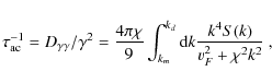
where
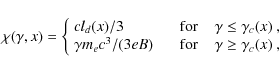
where x indicates the spatial location in the downstream,
| |
= | 
|
(7) |
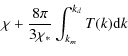
![$\displaystyle \frac{4\pi \chi_*}{3}\int_{k_m}^{k_d}
\left[\frac{1}{k^2\chi_*^2+...
...}-\frac{2(k^2\chi_*^2-v_F^2)}
{(k^2\chi_*^2+v_F^2)^2}\right]k^2 S(k) {\rm d}k~,$](/articles/aa/full_html/2010/09/aa15169-10/img45.png)
|
where we have ignored the decay of incompressive motions. Then we have

|
(8) |
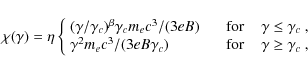
With the above treatment, we can study particle acceleration by compressive motions all the way to the shock front, which is different from the case studied by Fan et al. (2010), where only the subsonic phase with vF>u is considered. Near the shock front, we assume
![\begin{figure}
\par\includegraphics[width=9cm,clip]{15169fg1.eps}
\vspace*{4mm}
\end{figure}](/articles/aa/full_html/2010/09/aa15169-10/img51.png)
|
Figure 1:
Model fit to the spectrum of SNR RX J1713.7-3946. The TeV data is from Aharonian et al. (2007), the Fermi data is from Funk (2009), and the X-ray data is from Tanaka et al. (2008)
(Thanks to Jun Fang). The thick solid, dashed line and the thin solid,
dashed line in the upper panel correspond to the diffusive shock,
stochastic acceleration model, and the model with an exponential, more
gradual cutoff in the electron distribution, respectively. The low and
high-energy spectral hump are produced by relativistic electrons
through the synchrotron and inverse Comptonization process,
respectively. The lower panels show the normalized residuals. From top to bottom,
they are for the model with an exponential and more gradual cutoff, the
DSA, and SA model. For the model with a gradual cutoff, the X-ray
errors have been artificially increased by a factor of 2 to
improve the fit. The reduced |
| Open with DEXTER | |
![\begin{figure}
\par\includegraphics[width=8.5cm,clip]{15169fg2.eps}
\vspace*{3mm}
\end{figure}](/articles/aa/full_html/2010/09/aa15169-10/img52.png)
|
Figure 2: Probability density function of model parameters normalized at the peak value. Different line types correspond to different models as explained in Fig. 1 and the text. |
| Open with DEXTER | |
3 Discussion
The SA model (Fig. 1) predicts a higher hard X-ray flux than the DSA model since the diffusion coefficient of the DSA model has a stronger dependence on the electron energies leading to a sharper high-energy cutoff. The electron distribution in the SA model includes contributions from broad regions in the downstream, which also makes the overall electron distribution broader. Future observations with NuSTAR and HXMT may be able to distinguish these two models.
In actual turbulent astrophysical shocks, both the DSA and SA mechanisms may contribute to the electron acceleration (Bykov & Toptygin 1993; Achterberg 1990). The distinction between the two resides in the dissipation structure (Berezhko & Krymsky 1988). Supersonic shock fronts dominate the acceleration in the DSA model. The SA model dominates in the subsonic phase. It is possible that the shock downstream of SNR RX 1713.7-3946 has both a supersonic and subsonic phase turbulence with the former closer to the shock front. The electron acceleration is therefore a continuous process in the turbulent downstream. In the SA model of this paper, we intentionally remove the DSA by requiring that the compressive waves be subsonic in the downstream. A self-consistent treatment of the turbulence evolution in the shock downstream is needed for particle acceleration near astrophysical shock fronts.
All the models appear to systematically underproduce ![]() -ray flux in the Fermi energy band and overproduce flux near 10 TeV. The latter could be
caused by inhomogeneities of the background magnetic field, which implies lower
cutoff energy of the electron distribution and less high-energy
-ray flux in the Fermi energy band and overproduce flux near 10 TeV. The latter could be
caused by inhomogeneities of the background magnetic field, which implies lower
cutoff energy of the electron distribution and less high-energy ![]() -ray
flux (Tanaka et al. 2008). The former requires a broader electron distribution from the
GeV to TeV energy range. A combination of DSA and SA model with the former
dominating the higher energy particle acceleration and the latter enhancing
the lower energy ones may address this issue. Such a scenario is possible
if both supersonic and subsonic turbulence are produced by the supernova
shock (Bykov & Toptygin 1993; Berezhko & Krymsky 1988).
Contributions to GeV-TeV emission from decay of neutral pions
produced by inelastic collisions of relativistic protons with the
background ions may also explain these residuals. However, as shown by
Ellision et al. (2010) and Katz & Waxman (2008), relativistic protons can not be the
dominant TeV emission component (Zirakashvili & Aharonian 2010). Including this
component is beyond the scope of the current investigation but may give
a good constraint on the relative acceleration efficiency of
relativistic electrons and protons (Katz & Waxman 2008).
-ray
flux (Tanaka et al. 2008). The former requires a broader electron distribution from the
GeV to TeV energy range. A combination of DSA and SA model with the former
dominating the higher energy particle acceleration and the latter enhancing
the lower energy ones may address this issue. Such a scenario is possible
if both supersonic and subsonic turbulence are produced by the supernova
shock (Bykov & Toptygin 1993; Berezhko & Krymsky 1988).
Contributions to GeV-TeV emission from decay of neutral pions
produced by inelastic collisions of relativistic protons with the
background ions may also explain these residuals. However, as shown by
Ellision et al. (2010) and Katz & Waxman (2008), relativistic protons can not be the
dominant TeV emission component (Zirakashvili & Aharonian 2010). Including this
component is beyond the scope of the current investigation but may give
a good constraint on the relative acceleration efficiency of
relativistic electrons and protons (Katz & Waxman 2008).
4 Conclusions
With recent high spectral-resolution observations of SNR RX 1713.7-3946 in X-rays andThis work is supported in part by the SOLAIRE research and training network at the University of Glasgow (MTRN-CT-2006-035484), the National Science Foundation of China (grants 10963004 and 10778702), Yunnan Provincial Science Foundation of China (grant 2008CD061) and SRFDP of China (grant 20095301120006). S.L. thanks Eduard Kontar for helpful discussion. Q.Y. thanks Jie Liu for helping to develop the MCMC code adapted from the COSMOMC code of Lewis & Bridle (2002).
References
- Achterberg, A. 1990, A&A, 231, 251 [NASA ADS] [Google Scholar]
- Aharonian, F. A., Akhperjanian, A. G., Bazer-Bachi, A. R., et al. 2006, A&A, 449, 223 [NASA ADS] [CrossRef] [EDP Sciences] [Google Scholar]
- Aharonian, F., Akhperjanian, A. G., Bazer-Bachi, A. R., et al. 2007, A&A, 464, 235 [Google Scholar]
- Becker, P. A., Le, T., & Demer, C. D. 2006, ApJ, 647, 539B [Google Scholar]
- Berezhko, E. G. 1996, Astropart. Phys., 5, 367 [NASA ADS] [CrossRef] [Google Scholar]
- Berezhko, E. G., & Krymsky, G. F. 1988, Sov. Phys. Usp., 31, 27 [Google Scholar]
- Blasi, P. 2010, MNRAS, 402, 2807 [NASA ADS] [CrossRef] [Google Scholar]
- Butt, Y. M. 2009, Nature, 460, 701 [NASA ADS] [CrossRef] [PubMed] [Google Scholar]
- Bykov, A. M., & Toptygin, I. N. 1993, Phys. Usp., 36, 1020 [Google Scholar]
- Cassam-Chenaï, G., Decourchelle, A., Ballet, J., et al. 2004, A&A, 427, 199 [NASA ADS] [CrossRef] [EDP Sciences] [Google Scholar]
- Cowsik, R., & Sarkar, S. 1984, MNRAS, 207, 745 [NASA ADS] [Google Scholar]
- Drury, L. 1983, SSRv, 36, 57 [Google Scholar]
- Drury, L. 1991, MNRAS, 251, 340 [NASA ADS] [Google Scholar]
- Ellison, D. C., Patnaude, D. J., Slane, P., & Raymond, J. 2010, ApJ, 712, 287 [NASA ADS] [CrossRef] [Google Scholar]
- Fan, Z. H., Liu, S. M., & Fryer, C. L. 2010, MNRAS, 406, 1337 [NASA ADS] [Google Scholar]
- Forman, M. A., & Drury, L. O. 1983, ICRC, 2, 267 [Google Scholar]
- Funk, S. 2009, Fermi Symp. [Google Scholar]
- Gamerman, D. 1997, Markov Chain Monte Carlo: Stochastic Simulation for Bayesian Inference (London: Chapman and Hall) [Google Scholar]
- Katz, B., & Waxman, E. 2008, JCAP, 01, 018 [NASA ADS] [CrossRef] [Google Scholar]
- Kolmogorov A. 1941, Dokl. Akad. Nauk SSSR, 30, 301 [Google Scholar]
- Kraichnan 1965, Phys. Fluids, 8, 1385 [Google Scholar]
- Lewis, A., & Bridle, S. 2002, Phys. Rev. D 66, 103511 [NASA ADS] [CrossRef] [Google Scholar]
- Liu, S. M., Fan, Z. H., Fryer, C. L., Wang, J. M., & Li, H. 2008, ApJ, 683, L163 [NASA ADS] [CrossRef] [Google Scholar]
- MacKay, D. 2003 Information Theory, Inference, and Learning Algorithms, (Cambridge University Press) [Google Scholar]
- Neal, R. M. 1993 Probabilistic Inference Using Markov Chain Monte Carlo Methods, Technical Report CRG-TR-93-1, Department of Computer Science, University of Toronto [Google Scholar]
- Park, B. T., & Petrosian, V. 1995, ApJ, 446, 699 [NASA ADS] [CrossRef] [Google Scholar]
- Plaga, R. 2008, NewA, 13, 73 [Google Scholar]
- Porter, T. A., Moskalenko, I. V., & Strong, A. W. 2006, ApJ, 648, L29 [NASA ADS] [CrossRef] [Google Scholar]
- Ptuskin, V. S. 1988, Soviet Astron. Lett., 14, 255 [NASA ADS] [Google Scholar]
- Takahashi, T., Tanaka, T., Uchiyama, Y., et al. 2008, PASJ, 60, 131 [Google Scholar]
- Tanaka, T., Uchiyama, Y., Aharonian, F. A., et al. 2008, ApJ, 685, 988 [NASA ADS] [CrossRef] [Google Scholar]
- Toptygin, I. N. 1980, SSRv, 26, 157 [Google Scholar]
- Uchiyama, Y., Aharonian, F. A., Tanaka, T., et al. 2007, Nature, 449, 576 [NASA ADS] [CrossRef] [PubMed] [Google Scholar]
- Zirakashvili, V. N., & Aharonian, F. A. 2007, A&A, 465, 695 [NASA ADS] [CrossRef] [EDP Sciences] [Google Scholar]
- Zirakashvili, V. N., & Aharonian, F. A. 2010, ApJ, 708, 965 [NASA ADS] [CrossRef] [Google Scholar]
Footnotes
- ... 2
![[*]](/icons/foot_motif.png)
- Given the complexity of the instrumental background and calibration, and unknowns, such as the estimated cosmic X-ray background, such an artificial increase may well be reasonable.
- ... turbulence
- Here we adopt the formula given by Bykov & Toptygin (1993), which gives an acceleration rate a factor of 2 lower than that of Ptuskin (1988).
- ... necessary
- At the point, where vF=u, the compressive wave intensity used here is 3 times lower than in Fan et al. (2010).
All Figures
|
|
Figure 1:
Model fit to the spectrum of SNR RX J1713.7-3946. The TeV data is from Aharonian et al. (2007), the Fermi data is from Funk (2009), and the X-ray data is from Tanaka et al. (2008)
(Thanks to Jun Fang). The thick solid, dashed line and the thin solid,
dashed line in the upper panel correspond to the diffusive shock,
stochastic acceleration model, and the model with an exponential, more
gradual cutoff in the electron distribution, respectively. The low and
high-energy spectral hump are produced by relativistic electrons
through the synchrotron and inverse Comptonization process,
respectively. The lower panels show the normalized residuals. From top to bottom,
they are for the model with an exponential and more gradual cutoff, the
DSA, and SA model. For the model with a gradual cutoff, the X-ray
errors have been artificially increased by a factor of 2 to
improve the fit. The reduced |
| Open with DEXTER | |
| In the text | |
|
|
Figure 2: Probability density function of model parameters normalized at the peak value. Different line types correspond to different models as explained in Fig. 1 and the text. |
| Open with DEXTER | |
| In the text | |
Copyright ESO 2010
Current usage metrics show cumulative count of Article Views (full-text article views including HTML views, PDF and ePub downloads, according to the available data) and Abstracts Views on Vision4Press platform.
Data correspond to usage on the plateform after 2015. The current usage metrics is available 48-96 hours after online publication and is updated daily on week days.
Initial download of the metrics may take a while.