| Issue |
A&A
Volume 517, July 2010
|
|
|---|---|---|
| Article Number | L9 | |
| Number of page(s) | 3 | |
| Section | Letters | |
| DOI | https://doi.org/10.1051/0004-6361/201014362 | |
| Published online | 13 August 2010 | |
LETTER TO THE EDITOR
The H-test probability distribution revisited: improved sensitivity
O. C. de Jager1,3 - I. Büsching1,2
1 - Unit for Space Physics, School of
Physics, North-West University, 2520 Potchefstroom, South Africa
2 -
Centre for High Performance Computing (CHPC), CSIR Campus, 15 Lower Hope St. Rosebank, Cape Town, South Africa
3 -
South African Department of Science & Technology and National Research Foundation
Reseach Chair: Astrophysics & Space Science, South Africa
Received 5 March 2010 / Accepted 28 May 2010
Abstract
Aims. To provide a significantly improved probability distribution for the H-test for periodicity in X-ray and ![]() -ray arrival times, which is already extensively used by the
-ray arrival times, which is already extensively used by the ![]() -ray
pulsar community. Also, to obtain an analytical probability
distribution for stacked test statistics in the case of a search for
pulsed emission from an ensemble of pulsars where the significance per
pulsar is relatively low, making individual detections insignificant on
their own. This information is timely given the recent rapid discovery
of new pulsars with the Fermi-LAT t
-ray
pulsar community. Also, to obtain an analytical probability
distribution for stacked test statistics in the case of a search for
pulsed emission from an ensemble of pulsars where the significance per
pulsar is relatively low, making individual detections insignificant on
their own. This information is timely given the recent rapid discovery
of new pulsars with the Fermi-LAT t ![]() -ray telescope.
-ray telescope.
Methods. Approximately 1014 realisations of the H-statistic (H) for random (white) noise is calculated from a random number generator for which the repetition cycle is ![]() 1014. From these numbers the probability distribution P(>H) is calculated.
1014. From these numbers the probability distribution P(>H) is calculated.
Results. The distribution of H is found to be exponential with parameter
![]() so that the cumulative probability distribution
so that the cumulative probability distribution
![]() .
If we stack independent values for H, the sum of K such values would follow the Erlang-K distribution with parameter
.
If we stack independent values for H, the sum of K such values would follow the Erlang-K distribution with parameter ![]() for which the cumulative probability distribution is also a simple analytical expression.
for which the cumulative probability distribution is also a simple analytical expression.
Conclusions. Searches for weak pulsars with unknown pulse
profile shapes in the Fermi-LAT, Agile or other X-ray data bases should
benefit from the H-test since it is known to be powerful
against a broad range of pulse profiles, which introduces only a single
statistical trial if only the H-test is used. The new
probability distribution presented here favours the detection of weaker
pulsars in terms of an improved sensitivity relative to the previously
known distribution.
Key words: methods: statistical - pulsars: general
1 Introduction
When searching for a periodic signal in X-ray orde Jager et al. (1989, hereafter DSR) reviewed the general class of Beran statistics (Beran 1969), from which the most general test statistics such as
Pearson's ![]() ,
Rayleigh and Z2m statistics are derived, and from within this class they derived the
well known H-test for X-ray and
,
Rayleigh and Z2m statistics are derived, and from within this class they derived the
well known H-test for X-ray and ![]() -ray Astronomy.
-ray Astronomy.
The probability distribution of the H-test statistic as given by DSR
was derived from Monte Carlo simulations employing ![]() 108 simulations. The computational power and random number
simulators on typical IBM machines during the 1980's had limited ranges of applicability and the H-test suffered
accordingly. For values of H<23 we found that the probability distribution was exponential with parameter
108 simulations. The computational power and random number
simulators on typical IBM machines during the 1980's had limited ranges of applicability and the H-test suffered
accordingly. For values of H<23 we found that the probability distribution was exponential with parameter
![]() (or 0.4),
whereas a hard tail developed for H>23, which resulted in a significant compromise in sensitivity.
(or 0.4),
whereas a hard tail developed for H>23, which resulted in a significant compromise in sensitivity.
The old version of the H-test probability distribution is already extensively used by e.g. the Fermi-LAT Collaboration for pulsar searches (e.g. Abdo et al. 2009; and Weltevrede et al. 2010), and from this paper it will become clear that the significances assigned to pulsar detections (or non-detections) may be too conservative, so that some pulsars may be missed, especially when many trial periods are involved, so that large values of the H-statistic are required for a significant detection. In this Letter we notify the community that all previous published significances from the H-test should be reassessed, based on the new improved distribution presented below. Before we do so, we first briefly review the origin and properties of the H-test.
2 The Beran class of test statistics - towards the H-test
Let ![]() be the pulsar phase measured on the interval
be the pulsar phase measured on the interval ![]() ,
so that a full rotation corresponds to
,
so that a full rotation corresponds to ![]() .
Assuming noise (e.g. from cosmic rays) are also present such that the pulsed fraction is
.
Assuming noise (e.g. from cosmic rays) are also present such that the pulsed fraction is ![]() .
Let
.
Let
![]() be the observed line-of-sight
pulse profile in the absence of noise. The case p=0 then corresponds to no signal (pure noise), whereas p=1 corresponds to no noise (pure pulsed signal). The observed light curve
be the observed line-of-sight
pulse profile in the absence of noise. The case p=0 then corresponds to no signal (pure noise), whereas p=1 corresponds to no noise (pure pulsed signal). The observed light curve ![]() can then be represented as a mixing of the noise and signal distributions
(see Eq. (2) of DSR 1989)
can then be represented as a mixing of the noise and signal distributions
(see Eq. (2) of DSR 1989)
|
(1) |
The general form of the Beran statistic is given by Beran (1969) in the form (see also DSR 1989)
It is thus clear that the Beran statistic measures the integrated squared distance between the pulse profile and uniformity, so that if
It was noted by DSR that by replacing ![]() with a density estimator
with a density estimator
![]() based on the observed folded phases
based on the observed folded phases ![]() ,
we retrieve test statistics specific to the kernel of
the density estimator.
Selecting the Fourier series
estimator
,
we retrieve test statistics specific to the kernel of
the density estimator.
Selecting the Fourier series
estimator ![]() with m harmonics (see Eq. (5) of DSR) as representative of the light curve,
results in the well-known Z2m given the proper normalisation (Eq. (7) of DSR)
with m harmonics (see Eq. (5) of DSR) as representative of the light curve,
results in the well-known Z2m given the proper normalisation (Eq. (7) of DSR)
|
(3) |
Since
The main problem raised by DSR is that we do not know a-priori the optimal number of harmonics to select. In the case of the popular Z2m test, the optimal number of harmonics would depend on X and the pulse profile shape.
The rationale behind the H-test was to find a consistent estimator for ![]() where the
number of harmonics m is not chosen
subjectively by the observer, since selecting a number of m values for Z2m, until a pleasing result is obtained, may
lead to a false detection, given the difficulty to keep track of the number of trials involved.
where the
number of harmonics m is not chosen
subjectively by the observer, since selecting a number of m values for Z2m, until a pleasing result is obtained, may
lead to a false detection, given the difficulty to keep track of the number of trials involved.
Hart (1985) derived a technique to obtain the optimal number of harmonics M such that the
mean integrated squared error (MISE) between the Fourier series estimator
![]() and the
true unknown light curve shape is a minimum (see DSR for a review). Thus,
and the
true unknown light curve shape is a minimum (see DSR for a review). Thus,
![]() would give the best Fourier series representation of the true pulse profile, given the constraints
imposed by the statistics and inherent pulsed fraction. Since the minimum of the MISE involves the finding of
a maximum quantity over all harmonics m, DSR redefined this maximal (optimal) quantity in terms of the
so-called H-test statistic (named after Hart):
would give the best Fourier series representation of the true pulse profile, given the constraints
imposed by the statistics and inherent pulsed fraction. Since the minimum of the MISE involves the finding of
a maximum quantity over all harmonics m, DSR redefined this maximal (optimal) quantity in terms of the
so-called H-test statistic (named after Hart):
|
(4) |
Uniformity would correspond to low values of M and also low values of H, whereas large values of Z2M (relatively strong pulsed signal) corresponds to large values of H. Subtracting 4M and adding 4 (to ensure positive values of H only) effectively limits the variance of H in the absence of a pulsed signal. It is clear that the H test represents a rescaled version of the Z2m test: if M=1, then we retrieve the well-known Rayleigh test. DSR have shown that this test is powerful against a wide range of alternatives, which makes this test attractive if the pulse profile shape is not known a priori.
To give an example of how H and M depend on the abovementioned significance
![]() given
real data, we selected archival photon arrival times from the public
Fermi-LAT data base from the Vela pulsar direction, with events
selected according to the Fermi-LAT point spread function, but with
energies >500 MeV. Folding these phases with the given
contemporary spin parameters of Vela reveals a pulsed fraction of
given
real data, we selected archival photon arrival times from the public
Fermi-LAT data base from the Vela pulsar direction, with events
selected according to the Fermi-LAT point spread function, but with
energies >500 MeV. Folding these phases with the given
contemporary spin parameters of Vela reveals a pulsed fraction of
![]() ,
i.e.
nearly 100% and from N=600 events
(4 days integration)
we already obtain M=20.
By adding randomly generated events (i.e. uniformly distributed pulse
phases) to the signal events we effectively reduce p and hence X, so that H
and M should also decrease accordingly. Figure 1 shows how H and M relates to X: For X>3 (stronger than a
,
i.e.
nearly 100% and from N=600 events
(4 days integration)
we already obtain M=20.
By adding randomly generated events (i.e. uniformly distributed pulse
phases) to the signal events we effectively reduce p and hence X, so that H
and M should also decrease accordingly. Figure 1 shows how H and M relates to X: For X>3 (stronger than a
![]()
![]() signal) we see that H scales with X2, with H=1.9X2, whereas the
optimal M is already >10 for X>7.
signal) we see that H scales with X2, with H=1.9X2, whereas the
optimal M is already >10 for X>7.
![\begin{figure}
\par\includegraphics[width=8 cm,clip]{psqrtN.EPS}
\end{figure}](/articles/aa/full_html/2010/09/aa14362-10/img34.png)
|
Figure 1:
The dependence of H and M on the approximate skymap significance X for
|
| Open with DEXTER | |
This figure is also quite useful to see what typical H and M values we may expect for a typical Vela-like pulsar if we know the strength of the signal as derived from a point source on the skymap, and assuming the excess is due to such a pulsed signal.
3 The revised probability distribution of H for uniformity
The calculations were performed on the Institutional Cluster of the North-West
University, Potchefstroom campus. To parallelize the computations, we used the
RngStream package (L'Ecuyer 2002), which guarantees independent, non-overlapping
substreams of random numbers. The repetition cycle for this random number generator is
![]() ,
which is certainly large enough for our purposes. A total of
,
which is certainly large enough for our purposes. A total of
![]() samples were
calculated in this way.
samples were
calculated in this way.
In the case of large statistics (N>100) we do not need to simulate individual arrival times directly
(see the approximate correction factors in Figs. 1 and 2 of DSR in the case of low
statistics - N<100), so that we only need to simulate the Z2m statistics directly:
since Z2m is the sum of m ![]() -statistics, we can simulate a
-statistics, we can simulate a ![]() statistic
directly from a uniformly distributed random number
statistic
directly from a uniformly distributed random number
![]() by taking the transformation
by taking the transformation ![]() and adding these
numbers to give Z2m. This speeds up the process considerably.
A total of
and adding these
numbers to give Z2m. This speeds up the process considerably.
A total of
![]() values of H were simulated in this way and the results
are shown in Fig. 2. The distribution is everywhere consistent with an exponential
distribution with parameter
values of H were simulated in this way and the results
are shown in Fig. 2. The distribution is everywhere consistent with an exponential
distribution with parameter
![]() (or 0.4), except for H>70 where a downturn
relative to the 0.4 index is possibly seen.
DSR arrived at the same
precise value of
(or 0.4), except for H>70 where a downturn
relative to the 0.4 index is possibly seen.
DSR arrived at the same
precise value of
![]() for small values of H (i.e. less than 23)
since the random number generator used by DSR did not yet reach the limit of its random cycle
for the number of simulations required to reach
for small values of H (i.e. less than 23)
since the random number generator used by DSR did not yet reach the limit of its random cycle
for the number of simulations required to reach ![]() (with a relatively small error on the
corresponding probability) and should therefore reveal the same
result as ours for H<23.
(with a relatively small error on the
corresponding probability) and should therefore reveal the same
result as ours for H<23.
It is thus clear that the probability distribution of the
H-statistic
can be conservatively described by the simple formula
| (5) |
![\begin{figure}
\par\includegraphics[width=8 cm,clip]{h-statistic_2.EPS}
\end{figure}](/articles/aa/full_html/2010/09/aa14362-10/img42.png)
|
Figure 2:
The distribution of the H-statistic derived from
|
| Open with DEXTER | |
4 Incoherent stacking
Suppose we analysed the data from K pulsars, or, K independent observations of the same pulsar, where the effect of e.g. unrecorded glitches excluded the possibility of analysing all the data as one single coherent set of arrival times. In this case we want to see if there is a net signal represented by K values of the H-statistic. Suppose we arrive at a set of K such values of H, given by Hi, i=1, ...,K.
Since we have shown (to the probability level of ![]() 10-14) that the
H-statistic follows that of an exponential distribution with parameter
10-14) that the
H-statistic follows that of an exponential distribution with parameter
![]() ,
we can stack these test statistics through the sum
,
we can stack these test statistics through the sum

|
(6) |
which is known to follow the Erlang-K distribution with parameter
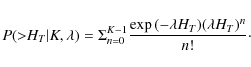
|
(7) |
5 Conclusions
For M=1 we retrieve the well-known Rayleigh test, with the exception that the parameter for
the exponential distribution has been reduced from
![]() (for the Rayleigh test)
to
(for the Rayleigh test)
to
![]() for the H-test. This slight loss of sensitivity is the effect of the
number of trials taken implicitly into account as a result of the search through m within the H-test.
for the H-test. This slight loss of sensitivity is the effect of the
number of trials taken implicitly into account as a result of the search through m within the H-test.
Finally, it is clear that the corrected distribution of the H-statistic follows a simple
exponential with parameter
![]() and evaluation of results for H>23 (i.e. the 10-4 significance
level) would yield more significant results compared to the old distribution presented by DSR.
For example, for H=50 a probability of
and evaluation of results for H>23 (i.e. the 10-4 significance
level) would yield more significant results compared to the old distribution presented by DSR.
For example, for H=50 a probability of
![]() is typically quoted in the literature,
whereas the true probability for uniformity is actually
is typically quoted in the literature,
whereas the true probability for uniformity is actually
![]() - already a factor 20 smaller.
- already a factor 20 smaller.
A Fermi-LAT example of the Vela pulsar (>500 MeV) shows clearly values for M up to 20 for ``skymap'' significances
![]() ,
whereas H scales with
,
whereas H scales with
![]() as expected for Beran-type tests. The scaling H=1.9X2 can be used to predict H-test statistics for Vela-like pulsars above 500 MeV if we assume the excess on the skymap is all pulsed.
as expected for Beran-type tests. The scaling H=1.9X2 can be used to predict H-test statistics for Vela-like pulsars above 500 MeV if we assume the excess on the skymap is all pulsed.
The hard tail of the distribution beyond H>23 presented by DSR probably arose from the repetition cycle of
the random number generator used in those days, so that the same fluctuations at large H values were repeated
given the finite cycle length of the generator used. In this case we however used a generator with a cycle time
much longer than 1014, in which case we did not see the repetition of outliers as a result of a
finite cycle length. Confirmation of the possible break (i.e. downturn) in the probability distribution at H>70 requires extensive simulations beyond
![]() and is beyond the scope of this paper.
and is beyond the scope of this paper.
The authors are grateful for partial financial support granted to them by the South African National Research Foundation (NRF) and by the Meraka Institute as part of the funding for the South African Centre for High Performance Computing (CHPC).
References
- Abdo, A. A., Ackermann, M., Ajello, M., et al. 2009, Science, 325, 840 [NASA ADS] [CrossRef] [Google Scholar]
- Atwood, W. B., Ziegler, M., Johnson, R. P., & Baughman, B. M. 2006, ApJ, 652, L49 [NASA ADS] [CrossRef] [Google Scholar]
- Beran, R. J. 1969, Ann. Math. Stat., 40, 1196 [CrossRef] [Google Scholar]
- Buccheri, R., & de Jager, O. C. 1989, in NATO ASI Workshop on Timing Neutron Stars, ed. H. Ögelman, & E. P. J. van den Heuvel (Dordrecht: Kluwer), 95 [Google Scholar]
- de Jager, O. C., Swanepoel, J. W. H., & Raubenheimer, B. C. 1989, A&A, 221, 180 (DSR) [NASA ADS] [Google Scholar]
- Hart, J. D. 1985, J. Statist. Comput. Simul., 21, 95 [CrossRef] [Google Scholar]
- Leemis, L. M., & McQueston, J. T. 2008, American Statistician, 62, 45 [Google Scholar]
- L'Ecuyer, P., Simard, R., Chen, E. J., & Kelton, W. D. 2002, Operations Res., 50, 1073 [CrossRef] [Google Scholar]
- Weltevrede, P., Abdo, A. A., Ackermann, M., et al. 2010, ApJ, 708, 1426 [NASA ADS] [CrossRef] [Google Scholar]
All Figures
|
|
Figure 1:
The dependence of H and M on the approximate skymap significance X for
|
| Open with DEXTER | |
| In the text | |
|
|
Figure 2:
The distribution of the H-statistic derived from
|
| Open with DEXTER | |
| In the text | |
Copyright ESO 2010
Current usage metrics show cumulative count of Article Views (full-text article views including HTML views, PDF and ePub downloads, according to the available data) and Abstracts Views on Vision4Press platform.
Data correspond to usage on the plateform after 2015. The current usage metrics is available 48-96 hours after online publication and is updated daily on week days.
Initial download of the metrics may take a while.