| Issue |
A&A
Volume 517, July 2010
|
|
|---|---|---|
| Article Number | A79 | |
| Number of page(s) | 7 | |
| Section | Interstellar and circumstellar matter | |
| DOI | https://doi.org/10.1051/0004-6361/200913982 | |
| Published online | 11 August 2010 | |
Scattered H emission from a large translucent cloud G294-24
![[*]](/icons/foot_motif.png)
K. Lehtinen - M. Juvela - K. Mattila
Observatory, Tähtitorninmäki, PO Box 14, 00014, University of Helsinki, Finland
Received 29 December 2009 / Accepted 25 March 2010
Abstract
Aims. We study an undocumented large translucent
cloud, detected by means of its enhanced radiation in the SHASSA
(Southern H-Alpha Sky Survey Atlas) survey. We consider whether its
excess surface brightness can be explained by light scattered off the
dust grains in the cloud, or whether emission from in situ ionized gas
is required. In addition, we aim to determine the temperature of dust,
the mass of the cloud, and its possible star formation activity.
Methods. We compare the observed H![]() surface brightness of the cloud with predictions of a radiative
transfer model. We use the WHAM (Wisconsin H-Alpha Mapper) survey as a
source for the Galactic H
surface brightness of the cloud with predictions of a radiative
transfer model. We use the WHAM (Wisconsin H-Alpha Mapper) survey as a
source for the Galactic H![]() interstellar radiation field illuminating the cloud. Visual extinction
through the cloud is derived using 2MASS J, H,
and K band photometry. We use far-IR ISOSS
(ISO Serendipitous Survey), IRAS, and DIRBE data to study the thermal
emission of dust. The LAB (The Leiden/Argentine/Bonn Galactic HI
Survey) is used to study 21 cm HI emission associated with the
cloud.
interstellar radiation field illuminating the cloud. Visual extinction
through the cloud is derived using 2MASS J, H,
and K band photometry. We use far-IR ISOSS
(ISO Serendipitous Survey), IRAS, and DIRBE data to study the thermal
emission of dust. The LAB (The Leiden/Argentine/Bonn Galactic HI
Survey) is used to study 21 cm HI emission associated with the
cloud.
Results. Radiative transfer calculations of the
Galactic diffuse H![]() radiation indicate that the surface brightness of the cloud can be
explained solely by radiation scattered off dust particles in the
cloud. The maximum visual extinction through the cloud is about
1.2 mag. The cloud is found to be associated with
21 cm HI emission at a velocity
radiation indicate that the surface brightness of the cloud can be
explained solely by radiation scattered off dust particles in the
cloud. The maximum visual extinction through the cloud is about
1.2 mag. The cloud is found to be associated with
21 cm HI emission at a velocity ![]() -9 km s-1.
The total mass of the cloud is about 550-1000
-9 km s-1.
The total mass of the cloud is about 550-1000 ![]() .
There is no sign of star formation in this cloud. The distance of the
cloud is estimated from the Hipparcos data to be
.
There is no sign of star formation in this cloud. The distance of the
cloud is estimated from the Hipparcos data to be ![]() 100 pc.
100 pc.
Key words: ISM: clouds - dust, extinction - infrared: ISM
1 Introduction
del Burgo & Cambrésy (2006)
were the first to report on
detection of diffuse H![]() emission in a molecular cloud. They
detected an excess surface brightness over the cloud LDN1780
of
intensity
emission in a molecular cloud. They
detected an excess surface brightness over the cloud LDN1780
of
intensity ![]() 1-4 rayleigh
(one rayleigh (R) being equivalent to
1-4 rayleigh
(one rayleigh (R) being equivalent to
![]() erg cm-2 s-1 sr-1
at the wavelength
of H
erg cm-2 s-1 sr-1
at the wavelength
of H![]() emission). They interpreted the surface brightness as a
result of enhanced in situ cosmic ray ionization. However, Mattila
et al. (2007)
showed that the H
emission). They interpreted the surface brightness as a
result of enhanced in situ cosmic ray ionization. However, Mattila
et al. (2007)
showed that the H![]() surface
brightness observed in LDN1780 can be explained solely in terms of
scattered H
surface
brightness observed in LDN1780 can be explained solely in terms of
scattered H![]() radiation. In addition, Mattila et al. found
several other molecular clouds that had excess H
radiation. In addition, Mattila et al. found
several other molecular clouds that had excess H![]() emission
relative to the surroundings of the cloud. In some cases, a cloud was
not detected in H
emission
relative to the surroundings of the cloud. In some cases, a cloud was
not detected in H![]() images, although other physically similar
clouds do. These observations can be naturally explained in the
framework of scattered H
images, although other physically similar
clouds do. These observations can be naturally explained in the
framework of scattered H![]() radiation by varying the proportions
of general diffuse in situ H
radiation by varying the proportions
of general diffuse in situ H![]() emission either in front of or
behind the dust cloud.
emission either in front of or
behind the dust cloud.
While comparing the all-sky H![]() and 100
and 100 ![]() m
IRAS maps, we
noticed a large cloud visible in both maps. The Galactic coordinates
of the cloud are
m
IRAS maps, we
noticed a large cloud visible in both maps. The Galactic coordinates
of the cloud are ![]() ,
,
![]() .
The
maximum excess surface brightness of H
.
The
maximum excess surface brightness of H![]() is about 2.4 R. With
a size of about 1.4
is about 2.4 R. With
a size of about 1.4![]()
![]() 4.9
4.9![]() ,
the cloud is the largest
dust cloud visible in the light of scattered H
,
the cloud is the largest
dust cloud visible in the light of scattered H![]() emission known
to us. Hereafter the cloud is called G294-24.
emission known
to us. Hereafter the cloud is called G294-24.
2 Observations and calculations
![\begin{figure}
\par\includegraphics[width=15cm,clip]{13982fg1.eps}
\end{figure}](/articles/aa/full_html/2010/09/aa13982-09/img22.png)
|
Figure 1:
Map of visual extinction a) map of
644/677 nm continuum intensity, b)
map of IRAS 100 |
| Open with DEXTER | |
Dust grains in the cloud G294-24 are seen in the light of scattered and emitted radiation. In addition, dust grains cause extinction of light of those stars which are located behind the cloud. Atomic hydrogen gas in the cloud is expected to be seen in the 21 cm spin-flip line. We are studying these components by utilizing different data archives.
2.1 H
surface brightness
We obtained the H![]() data from the SHASSA (Southern H-Alpha Sky
Survey Atlas) survey (Gaustad et al. 2001), which is
incorporated into the all-sky composite map by Finkbeiner
(2003)
data from the SHASSA (Southern H-Alpha Sky
Survey Atlas) survey (Gaustad et al. 2001), which is
incorporated into the all-sky composite map by Finkbeiner
(2003)![]() . The data
were re-gridded into a regular grid in Galactic coordinate system,
using a pixel size of
. The data
were re-gridded into a regular grid in Galactic coordinate system,
using a pixel size of ![]() ,
which gives the
same pixel area as the original HEALPix data. The H
,
which gives the
same pixel area as the original HEALPix data. The H![]() data have
a spatial resolution of
data have
a spatial resolution of ![]() .
The intensities are given in
units of rayleigh (R).
.
The intensities are given in
units of rayleigh (R).
2.2 644/677 nm surface brightness
The SHASSA survey includes continuum images taken with a dual-band
(644 and 677 nm) notch filter. In the original SHASSA
survey, these
images were used to subtract continuum emission from the H![]() images.
In the case of dust clouds, these continuum images detect
diffuse interstellar radiation scattered off the dust clouds. With a
pixel size of 47.6
images.
In the case of dust clouds, these continuum images detect
diffuse interstellar radiation scattered off the dust clouds. With a
pixel size of 47.6
![]() ,
the low surface brightness of the cloud is
superimposed by numerous undersampled stars, which cannot be removed
by fitting the stars with the point spread function of the
instrument. To remove the stars, we replaced each map pixel with a
mean value over a
,
the low surface brightness of the cloud is
superimposed by numerous undersampled stars, which cannot be removed
by fitting the stars with the point spread function of the
instrument. To remove the stars, we replaced each map pixel with a
mean value over a ![]() pixel
area around the pixel in question,
using only those pixels that occupy the lowest 30% of the intensity
histogram. The resolution of the image was then about 7.2
pixel
area around the pixel in question,
using only those pixels that occupy the lowest 30% of the intensity
histogram. The resolution of the image was then about 7.2![]() .
Figure 1b
shows the continuum image after most of the stars
were removed. Some residuals remain in place of the brightest stars.
The intensity of the continuum surface brightness in SHASSA for the
644/677 nm filter is given in rayleigh units. This has been
scaled
for the purpose of background subtraction from the H
.
Figure 1b
shows the continuum image after most of the stars
were removed. Some residuals remain in place of the brightest stars.
The intensity of the continuum surface brightness in SHASSA for the
644/677 nm filter is given in rayleigh units. This has been
scaled
for the purpose of background subtraction from the H![]() filter
band. The physical units for the continuum surface brightness are
R/
filter
band. The physical units for the continuum surface brightness are
R/![]() and the value depends on the width of the filter. Thus, we
cannot compare the absolute intensities of the 644/677 nm and
H
and the value depends on the width of the filter. Thus, we
cannot compare the absolute intensities of the 644/677 nm and
H![]() images from the SHASSA survey.
images from the SHASSA survey.
2.3 IRAS/IRIS and ISOSS (ISO Serendipity Survey) far-IR data
We used the 100 ![]() m
IRIS data and the 170
m
IRIS data and the 170 ![]() m ISOSS data to
derive equilibrium temperature and column density of the ``big
classical'' dust grains in the cloud. IRIS data set
(Miville-Deschênes & Lagache 2005) is an
improved
version of the all-sky IRAS/ISSA data.
m ISOSS data to
derive equilibrium temperature and column density of the ``big
classical'' dust grains in the cloud. IRIS data set
(Miville-Deschênes & Lagache 2005) is an
improved
version of the all-sky IRAS/ISSA data.
The 170 ![]() m
slew data of the ISOPHOT instrument aboard the ISO
satellite were assembled into the ISOPHOT Serendipity Survey data set
by Stickel et al. (2007).
It covers
m
slew data of the ISOPHOT instrument aboard the ISO
satellite were assembled into the ISOPHOT Serendipity Survey data set
by Stickel et al. (2007).
It covers ![]() 15%
of the
sky, mapped with a grid size of 22
15%
of the
sky, mapped with a grid size of 22
![]() 4,
and a few slews cover our
cloud. The one that we used in our data analysis is shown
in Fig. 1c.
4,
and a few slews cover our
cloud. The one that we used in our data analysis is shown
in Fig. 1c.
2.4 COBE/DIRBE far-IR data
Because of the large size of the cloud, it is resolved in DIRBE data,
which have a beam size of about 0.7![]() .
We thus used DIRBE data at
100
.
We thus used DIRBE data at
100 ![]() m,
140
m,
140 ![]() m,
and 240
m,
and 240 ![]() m
to obtain another estimate
of the temperature and column density of the ``big classical'' dust
grains.
m
to obtain another estimate
of the temperature and column density of the ``big classical'' dust
grains.
2.5 Visual extinction
We compiled an extinction map of the cloud by applying the NICER (Near Infrared Color Excess Revised) method of Lombardi & Alves (2001), which is an optimized color excess technique using data in three bands simultaneously. Our data comprise J, H, andThe grid used in the extinction map is the same as that of the
H![]() map. The extinction value at each grid point is a weighted
mean of the individual extinctions of stars obtained by using a
Gaussian with a width of
map. The extinction value at each grid point is a weighted
mean of the individual extinctions of stars obtained by using a
Gaussian with a width of ![]() as a weighting function.
as a weighting function.
2.6 Hipparcos data
Owing to the large size and low extinction of the cloud, the Hipparcos
data (ESA 1997)
enable us to estimate the distance of the cloud. We collected Hipparcos
data over ![]() area towards the cloud.
The intrinsic colors of stars as a function of spectral and luminosity
class were used to derive a color excess E(B-V)
for each Hipparcos
star in the area.
area towards the cloud.
The intrinsic colors of stars as a function of spectral and luminosity
class were used to derive a color excess E(B-V)
for each Hipparcos
star in the area.
2.7 Hydrogen 21 cm line emission data
The ``The Leiden/Argentine/Bonn (LAB) Survey of Galactic HI'' dataset (Kalberla et al. 2005; Bajaja et al. 2005) was used to search for hydrogen emission related to the cloud. The angular resolution of the LAB survey is2.8 Subtraction of background sky
When studying extinction, scattering and emission associated solely
with the cloud G294-24, we need to subtract the background, determined
in the immediate vicinity of G294-24. Figure 1 shows the
circular area that was used to estimate the background for each
dataset. The background values of 100 ![]() m intensity, extinction
AV, and H
m intensity, extinction
AV, and H![]() brightness are about 4.1 MJy sr-1,
0.5 mag, and 1.0 R, respectively.
brightness are about 4.1 MJy sr-1,
0.5 mag, and 1.0 R, respectively.
3 Results
3.1
Comparison of H,
I(100  m),
AV, and 644/677 nm
maps
m),
AV, and 644/677 nm
maps
Inspection of Fig. 1
shows that the oval cloud at the center
of the images is visible in extinction (panel a), in scattered light
caused by dust (panel b), and in thermal emission by dust
(panel c). The same cloud is also seen in the light of the H![]() line
(panel d). The maximum excess H
line
(panel d). The maximum excess H![]() surface brightness of the
cloud above the background is about 2.0 rayleighs (R), which is
similar to the brightness of the other H
surface brightness of the
cloud above the background is about 2.0 rayleighs (R), which is
similar to the brightness of the other H![]() scattering clouds,
1-3 R, as discovered by Mattila et al. (2007). We show
in Sect. 3.8 that the detected H
scattering clouds,
1-3 R, as discovered by Mattila et al. (2007). We show
in Sect. 3.8 that the detected H![]() radiation can be explained
solely in terms of scattered radiation.
radiation can be explained
solely in terms of scattered radiation.
In addition to the central oval and the SW leg that are seen
in the
AV data,
the H![]() map shows a blob-like structure at
coordinates
map shows a blob-like structure at
coordinates ![]() ,
,
![]() ,
which is not seen in any of
the other maps. The maximum surface brightness of the blob is about
7 R, and thus the blob cannot be scattered light (see
Sect. 3.8).
The emission must instead be in situ emission from hot,
ionized
gas, possibly unconnected to the G294-24 dust cloud. Similar small
size (
,
which is not seen in any of
the other maps. The maximum surface brightness of the blob is about
7 R, and thus the blob cannot be scattered light (see
Sect. 3.8).
The emission must instead be in situ emission from hot,
ionized
gas, possibly unconnected to the G294-24 dust cloud. Similar small
size (![]()
![]() )
H
)
H![]() enhancements at latitudes
enhancements at latitudes
![]() were reported by Reynolds et al. (2005)
in the northern sky. Many of them have no obvious embedded or
associated ionizing star. This is also the case for our H
were reported by Reynolds et al. (2005)
in the northern sky. Many of them have no obvious embedded or
associated ionizing star. This is also the case for our H![]() blob.
This H
blob.
This H![]() enhancement could be associated with a planetary
nebula, or be ionized by either a O or early B type
star, or a hot
evolved low-mass star (Reynolds et al. 2005). The
SIMBAD database does not list any of these kinds of objects within a
distance of 1
enhancement could be associated with a planetary
nebula, or be ionized by either a O or early B type
star, or a hot
evolved low-mass star (Reynolds et al. 2005). The
SIMBAD database does not list any of these kinds of objects within a
distance of 1![]() from the center of the blob. The nearest O or
early B type star in SIMBAD is the B2 type star CD-80 228
(
from the center of the blob. The nearest O or
early B type star in SIMBAD is the B2 type star CD-80 228
(
![]() ,
,
![]() ),
identified as EC 06387-8045, at a distance of
4.4 kpc (Kilkenny et al. 1995).
Association of the blob with the star CD-80 228 would mean
that the blob is located much further away than G294-24 (see
Sect. 3.5).
),
identified as EC 06387-8045, at a distance of
4.4 kpc (Kilkenny et al. 1995).
Association of the blob with the star CD-80 228 would mean
that the blob is located much further away than G294-24 (see
Sect. 3.5).
The correlation plots between H![]() ,
,
![]() m),
I(644 nm/677 nm), and AV
data are shown in Fig. 2,
after
subtracting the background values from each dataset. To correlate data
sets produced in a compatible way, both sets of data in panel
Fig. 2c
are from the original SHASSA survey (Gaustad
et al. 2001),
and analyzed as described above in
Sect. 2.2. The absolute intensity calibration performed by our
analysis method in Fig. 2c
is inaccurate, as indicated
by a calibration difference of a factor of two between the
Finkbeiner's (2003)
(WHAM calibrated) H
m),
I(644 nm/677 nm), and AV
data are shown in Fig. 2,
after
subtracting the background values from each dataset. To correlate data
sets produced in a compatible way, both sets of data in panel
Fig. 2c
are from the original SHASSA survey (Gaustad
et al. 2001),
and analyzed as described above in
Sect. 2.2. The absolute intensity calibration performed by our
analysis method in Fig. 2c
is inaccurate, as indicated
by a calibration difference of a factor of two between the
Finkbeiner's (2003)
(WHAM calibrated) H![]() data
(panels a and b) and H
data
(panels a and b) and H![]() data in panel c.
However, the linear relation in panel c supports the idea that
the H
data in panel c.
However, the linear relation in panel c supports the idea that
the H![]() intensity is also mainly scattered light. In the
following, our analysis of the H
intensity is also mainly scattered light. In the
following, our analysis of the H![]() surface brightness is based
solely on Finkbeiner's (2003)
data, because its
calibration is based on the accurately calibrated WHAM survey (Haffner
et al. 2003).
surface brightness is based
solely on Finkbeiner's (2003)
data, because its
calibration is based on the accurately calibrated WHAM survey (Haffner
et al. 2003).
3.2 Temperature and column density of dust
Equilibrium temperature of dust particles along the ISOSS slew was
derived from the ISOSS and IRIS far-IR data, after subtracting an
estimate of the background intensity, assumed to be a mean value over
the circular region shown in Fig. 1c. We assume a
frequency
dependence of ![]() for the emissivity index. The ISOSS data were
convolved to the resolution of the IRIS data, which is given by a
Gaussian
for the emissivity index. The ISOSS data were
convolved to the resolution of the IRIS data, which is given by a
Gaussian ![]() .
The temperature along the ISOSS slew (see
Fig. 1c)
is plotted in Fig. 3
as a solid line,
showing that the temperature decreases from
about 18.7 K at the
northern edge of the cloud to a minimum of
about 17.5 K at the
center.
.
The temperature along the ISOSS slew (see
Fig. 1c)
is plotted in Fig. 3
as a solid line,
showing that the temperature decreases from
about 18.7 K at the
northern edge of the cloud to a minimum of
about 17.5 K at the
center.
The 100 ![]() m
optical depth, derived with the formula
m
optical depth, derived with the formula
| (1) |
is shown in Fig. 3 as a dotted line. The maximum optical depth is
To determine the dust temperature from the DIRBE maps, we
first
subtracted the estimated background intensities from the DIRBE maps,
derived in the circular area shown in Fig. 1. The dust
temperature was then derived by fitting the 100 ![]() m,
140
m,
140 ![]() m,
and 240
m,
and 240 ![]() m
intensities with a modified black body having a
m
intensities with a modified black body having a
![]() emissivity
law. The minimum temperature of the cloud is
emissivity
law. The minimum temperature of the cloud is
![]()
![]() K,
in agreement with the minimum temperature derived
from ISOSS and IRAS data. It is obvious that we are unable to resolve
any possible colder condensations in the cloud due to the low
resolution of DIRBE data. Figure 4 shows a map of the
100
K,
in agreement with the minimum temperature derived
from ISOSS and IRAS data. It is obvious that we are unable to resolve
any possible colder condensations in the cloud due to the low
resolution of DIRBE data. Figure 4 shows a map of the
100 ![]() m
optical depth based on DIRBE data, derived
using Eq. (1).
m
optical depth based on DIRBE data, derived
using Eq. (1).
The total mass (gas plus dust) of the cloud was calculated
with
the formula
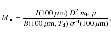
|
(2) |
where
![\begin{figure}
\par\includegraphics[width=7.5cm,clip]{13982fg2.eps}
\end{figure}](/articles/aa/full_html/2010/09/aa13982-09/img53.png)
|
Figure 2:
The observed H |
| Open with DEXTER | |
![\begin{figure}
\par\includegraphics[width=8cm,clip]{13982fg3.eps}
\end{figure}](/articles/aa/full_html/2010/09/aa13982-09/img55.png)
|
Figure 3:
Solid line: temperature of dust, |
| Open with DEXTER | |
![\begin{figure}
\par\includegraphics[width=8cm,clip]{13982fg4.eps}
\end{figure}](/articles/aa/full_html/2010/09/aa13982-09/img56.png)
|
Figure 4:
100 |
| Open with DEXTER | |
3.3 Visual extinction
The visual extinction map is shown in Fig. 1a. Maximum
visual extinction is ![]() 1.2 mag
over the background. The typical
error in the extinction map is 0.2 mag.
1.2 mag
over the background. The typical
error in the extinction map is 0.2 mag.
We can use the visual extinction to estimate the total
hydrogen column
density, ![]() .
As a starting point, we adopt
the value
.
As a starting point, we adopt
the value ![]() cm-2 mag-1
for
diffuse clouds (Bohlin et al. 1978), together
with
AV/E(B-V)=3.1
(``diffuse dust'') to obtain
cm-2 mag-1
for
diffuse clouds (Bohlin et al. 1978), together
with
AV/E(B-V)=3.1
(``diffuse dust'') to obtain
![]() cm-2 mag-1.
cm-2 mag-1.
The total cloud mass can then be derived with the formula
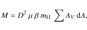
|
(3) |
where D is the cloud distance,
3.4 AV
versus  (100 m)
![\begin{figure}
\par\includegraphics[width=7.5cm,clip]{13982fg7.eps}
\end{figure}](/articles/aa/full_html/2010/09/aa13982-09/img62.png)
|
Figure 5:
Relation between 100 |
| Open with DEXTER | |
Figure 5
shows the relation between visual extinction and
100 ![]() m
optical depth, after the AV
map has been convolved to
the resolution of the DIRBE data. The slope of the fit gives the
emissivity
m
optical depth, after the AV
map has been convolved to
the resolution of the DIRBE data. The slope of the fit gives the
emissivity ![]() mag-1.
For a
mag-1.
For a
![]() emissivity
law, the emissivity at 200
emissivity
law, the emissivity at 200 ![]() m is
m is
![]() mag-1.
The observed value agrees with
theoretical values of
mag-1.
The observed value agrees with
theoretical values of ![]() m) for
diffuse interstellar
matter (Désert et al. 1990;
Dwek et al. 1997;
Cambrésy et al. 2001;
Li & Draine 2001;
see
Lehtinen et al. 2007
for a compilation of values of
m) for
diffuse interstellar
matter (Désert et al. 1990;
Dwek et al. 1997;
Cambrésy et al. 2001;
Li & Draine 2001;
see
Lehtinen et al. 2007
for a compilation of values of
![]() m)).
m)).
3.5 Distance based on Hipparcos data
Figure 6
shows E(B-V)
versus distance for the stars shown
in Fig. 1a.
Color excess E(B-V)
has been converted
into AV
by assuming a normal reddening law, AV/E(B-V)=3.1.
For
stars that are within the cloud area and have E(B-V)>0.1,
the
minimum distance is ![]() 100 pc.
Thus, we adopt a distance of
100 pc for G294-24, which is less than the distance of
150 pc to the
adjacent Chamaeleon region (Knude & Høg 1998).
100 pc.
Thus, we adopt a distance of
100 pc for G294-24, which is less than the distance of
150 pc to the
adjacent Chamaeleon region (Knude & Høg 1998).
3.6 HI emission line data
![\begin{figure}
\par\includegraphics[width=7.5cm,clip]{13982fg5.eps}
\end{figure}](/articles/aa/full_html/2010/09/aa13982-09/img67.png)
|
Figure 6: The reddening E(B-V) of Hipparcos stars as a function of their distances for the stars marked in Fig. 1a. The stars that are shown as filled circles are within the ellipse in Fig. 1a. The vertical line is at a distance of 100 pc. |
| Open with DEXTER | |
![\begin{figure}
\par\includegraphics[width=7.5cm,clip]{13982fg8.eps}
\end{figure}](/articles/aa/full_html/2010/09/aa13982-09/img68.png)
|
Figure 7:
Spectrum of 21 cm hydrogen line at the position |
| Open with DEXTER | |
![\begin{figure}
\par\includegraphics[width=7.5cm,clip]{13982fg9.eps}
\end{figure}](/articles/aa/full_html/2010/09/aa13982-09/img69.png)
|
Figure 8: Map of line area ([K km s-1]) of 21 cm HI emission from the cloud G294-24. The ellipse, which is the same as in Fig. 1, delineates the area used to determine the atomic hydrogen mass of the cloud. |
| Open with DEXTER | |
Figure 7
shows a HI spectrum from the LAB survey towards the
position ![]() ,
,
![]() .
Velocity-longitude diagrams
show that the strength of the narrow component at
.
Velocity-longitude diagrams
show that the strength of the narrow component at
![]() -9 km s-1
follows the intensity of the far-IR emission of
G294-24. The component at
-9 km s-1
follows the intensity of the far-IR emission of
G294-24. The component at ![]() 4 km s-1
is from gas in the
Galactic plane. We fit the spectrum in Fig. 7 with three
Gaussian functions, and use the fit as a template for fits at other
Galactic coordinates; the width of the narrow line at
4 km s-1
is from gas in the
Galactic plane. We fit the spectrum in Fig. 7 with three
Gaussian functions, and use the fit as a template for fits at other
Galactic coordinates; the width of the narrow line at
![]() -9 km s-1
is kept constant, and the velocities of the
narrow components at
-9 km s-1
is kept constant, and the velocities of the
narrow components at ![]() -9 km s-1
and
-9 km s-1
and ![]() 4 km s-1are
allowed to vary by
4 km s-1are
allowed to vary by ![]() 3 km s-1.
Figure 8
shows
a map of the line area of the narrow component at
3 km s-1.
Figure 8
shows
a map of the line area of the narrow component at
![]() -9 km s-1.
The oval G294-24 cloud and the SW leg are
seen. The blob, seen at coordinates
-9 km s-1.
The oval G294-24 cloud and the SW leg are
seen. The blob, seen at coordinates ![]() ,
,
![]() on
the H
on
the H![]() map, cannot be seen as a separate entity in the LAB
data, lending support to the idea that the blob is ionized gas. The
maximum of line area is located on the eastern side of the cloud, in
contrast to the maximum of 100
map, cannot be seen as a separate entity in the LAB
data, lending support to the idea that the blob is ionized gas. The
maximum of line area is located on the eastern side of the cloud, in
contrast to the maximum of 100 ![]() m optical depth, which is located
on the western side.
m optical depth, which is located
on the western side.
The column density (atoms per cm-2) of
atomic hydrogen can be
obtained from (see e.g., Verschuur 1974)
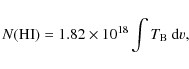
|
(4) |
where
The large-scale 12CO(J=1-0)
survey of the Chamaeleon region by
Mizuno et al. (2001)
shows a weak, isolated region near
the center of G294-24, seen only in the velocity range
2-6 km s-1. The integrated
intensity of 12CO(J=1-0)
emission towards the cloud is estimated to be ![]() 2 K km s-1(Fig. 1
of Mizuno et al.). The possible relation of the CO emission
with the cloud G294-24 has to be studied with observations of higher
angular resolution.
2 K km s-1(Fig. 1
of Mizuno et al.). The possible relation of the CO emission
with the cloud G294-24 has to be studied with observations of higher
angular resolution.
3.7 IRAS or 2MASS point sources
We checked the IRAS point source catalog for objects that have
spectral energy distribution typical of young stellar objects. There
are several 100 ![]() m
only sources in the cloud. They are probably
small cirrus structures seen as points sources by IRAS at 100
m
only sources in the cloud. They are probably
small cirrus structures seen as points sources by IRAS at 100 ![]() m,
and we do not consider them further here. The only source that has
fluxes measured at least at the two longest IRAS wavelengths is
IRAS 08048-8211, which was identified as a galaxy by Buta
(1995).
m,
and we do not consider them further here. The only source that has
fluxes measured at least at the two longest IRAS wavelengths is
IRAS 08048-8211, which was identified as a galaxy by Buta
(1995).
We compiled a color-color diagram (J-H versus H-K magnitudes) for all the stars with magnitude errors smaller than 0.05 mag at J, H, and K band. There is no star within the cloud area that exhibits a significant infrared excess above the color indices that can be explained by interstellar reddening.
Based on the non-existence of IRAS point sources and 2MASS objects with colors characteristic of young stellar objects, we conclude that the cloud is devoid of star formation.
3.8 Radiative transfer calculations
The maximum possible surface brightness of any Galactic dust cloud,
due to scattering, is limited by the average all-sky H![]() surface
brightness of
surface
brightness of ![]() 8 R.
Since the H
8 R.
Since the H![]() excess surface
brightness of G294-24 of
excess surface
brightness of G294-24 of ![]() 2.4 R
is well below this value, we
conclude that it can be explained solely by scattered radiation. To
verify this assumption, we simulated scattered H
2.4 R
is well below this value, we
conclude that it can be explained solely by scattered radiation. To
verify this assumption, we simulated scattered H![]() radiation
with Monte Carlo radiative transfer calculations (Mattila
1970; Juvela
& Padoan 2003;
Juvela
2005). We
used the WHAM Northern Sky Survey (Haffner
2003) to
derive the intensity of the northern H
radiation
with Monte Carlo radiative transfer calculations (Mattila
1970; Juvela
& Padoan 2003;
Juvela
2005). We
used the WHAM Northern Sky Survey (Haffner
2003) to
derive the intensity of the northern H![]() background sky illuminating
the model cloud. The missing southern sky
was recreated by assuming symmetry about the Galactic latitude and
longitude. The physical model of the cloud is a spherical, homogeneous
cloud with AV=1.2 mag
of visual extinction through the cloud
center. Properties of dust particles are based on Draine's
(2003)
``Milky Way'' dust model, with albedo a=0.67 and
asymmetry parameter g=0.5 at the wavelength of the H
background sky illuminating
the model cloud. The missing southern sky
was recreated by assuming symmetry about the Galactic latitude and
longitude. The physical model of the cloud is a spherical, homogeneous
cloud with AV=1.2 mag
of visual extinction through the cloud
center. Properties of dust particles are based on Draine's
(2003)
``Milky Way'' dust model, with albedo a=0.67 and
asymmetry parameter g=0.5 at the wavelength of the H![]() line.
For more details of applying Monte Carlo method to the scattering of
H
line.
For more details of applying Monte Carlo method to the scattering of
H![]() radiation, we refer to Mattila et al. (2007).
radiation, we refer to Mattila et al. (2007).
A general formula for the differential surface brightness of H![]() light
towards a dust cloud, measured over the brightness of the
adjacent sky, is
light
towards a dust cloud, measured over the brightness of the
adjacent sky, is
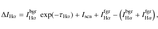
|
(5) |
where the first term on the right-hand side is the intensity of emission coming from behind the cloud attenuated by the optical depth through the cloud, the second term is the intensity of radiation scattered off the cloud, the third term is the intensity of emission between the cloud and the observer, and the term in parenthesis is the intensity of sky adjacent to the cloud. The radiative transfer calculations provide us with the value of
![\begin{figure}
\par\includegraphics[width=7.5cm,clip]{13982fg6.eps}
\end{figure}](/articles/aa/full_html/2010/09/aa13982-09/img76.png)
|
Figure 9:
Intensity of H |
| Open with DEXTER | |
|
(6) |
Figure 9 shows the observed intensity difference,
In addition, we used the above-mentioned model cloud in
radiative
transfer calculations of continuum radiation (Juvela & Padoan
2003), giving
us the surface brightness of the cloud at
far-infrared wavelengths. The interstellar radiation field surrounding
the cloud is taken from Mathis et al. (1983). Properties
of dust particles are based on Draine's (2003) ``Milky
Way'' dust model, not including stochastically heated dust grains.
The derived 100 ![]() m,
170
m,
170 ![]() m,
and 240
m,
and 240 ![]() m
maximum surface
brightnesses are about 12 MJy sr-1,
24 MJy sr-1, and
19 MJy sr-1, respectively. The
observed maximum surface
brightnesses above the background are about 13 MJy sr-1,
25 MJy sr-1, and
21 MJy sr-1, respectively. We
then
derived the dust temperature using the 100
m
maximum surface
brightnesses are about 12 MJy sr-1,
24 MJy sr-1, and
19 MJy sr-1, respectively. The
observed maximum surface
brightnesses above the background are about 13 MJy sr-1,
25 MJy sr-1, and
21 MJy sr-1, respectively. We
then
derived the dust temperature using the 100 ![]() m and
170
m and
170 ![]() m
maps. The minimum temperature is about 17.6 K, in good
agreement with
the temperature derived from IRIS and ISOSS data, of about
17.5 K
(see Sect. 3.2).
m
maps. The minimum temperature is about 17.6 K, in good
agreement with
the temperature derived from IRIS and ISOSS data, of about
17.5 K
(see Sect. 3.2).
4 Conclusions
We have studied the general properties of an undocumented large, nearby (distanceNote added in proof
After acceptance of our article Knude derived a distance of 217Acknowledgements26 pc for the cloud G294-24. Consequently, the mass of the cloud would be about 4.7 times higher than the value derived by us. No other conclusion of our article is affected by this new distance estimate. The method used by Knude is described in [arXiv:1006.3676] (Knude, J. 2010, A&A, submitted).
The work of K.L., M.J. and K.M. has been supported by the Finnish Academy through grants Nos. 1204415, 1210518, 1201269 and 117206, which is gratefully acknowledged. This publication makes use of data products from the Two Micron All Sky Survey, which is a joint project of the University of Massachusetts and the Infrared Processing and Analysis Center/California Institute of Technology, funded by the National Aeronautics and Space Administration and the National Science Foundation. This publication uses data from the Southern H-Alpha Sky Survey Atlas (SHASSA), which is supported by the National Science Foundation. The Wisconsin H-Alpha Mapper is funded by the National Science Foundation. This research has made use of SAOImage DS9, developed by Smithsonian Astrophysical Observatory
References
- Bajaja, E., Arnal, E. M., Larrarte, J. J., et al. 2005, A&A, 440, 767 [NASA ADS] [CrossRef] [EDP Sciences] [Google Scholar]
- Bohlin, R. C., Savage, B. D., & Drake, J. F. 1978, ApJ, 224, 132 [NASA ADS] [CrossRef] [Google Scholar]
- del Burgo, C., & Cambrésy, L. 2006, MNRAS, 368, 1463 [NASA ADS] [CrossRef] [Google Scholar]
- Buta, R. 1995, ApJS, 98, 739 [NASA ADS] [CrossRef] [Google Scholar]
- Cambrésy, L., Boulanger, F., Lagache, G., & Stepnik, B. 2001, A&A, 375, 999 [NASA ADS] [CrossRef] [EDP Sciences] [Google Scholar]
- Désert, F.-X., Boulanger, F., & Puget, J. L. 1990, A&A, 237, 215 [NASA ADS] [Google Scholar]
- Draine, B. 2003, ApJ, 598, 1017 [NASA ADS] [CrossRef] [Google Scholar]
- Dwek, E., Arendt, R. G., Fixsen, D. J., et al. 1997, ApJ, 475, 565 [NASA ADS] [CrossRef] [Google Scholar]
- ESA, The Hipparcos Cataloque 1997, ESA SP-1200 [Google Scholar]
- Finkbeiner, D. P. A. 2003, ApJS, 146, 407 [NASA ADS] [CrossRef] [Google Scholar]
- Gaustad, J. E., McCullough, P. R., Rosing, W., & Van Buren, D. 2001, PASP, 113, 1326 [NASA ADS] [CrossRef] [Google Scholar]
- Goerigk, W., Mebold, U., Reif, K., Kalberla, P. M. W., & Velden, L. 1983, A&A, 120, 63 [NASA ADS] [Google Scholar]
- Haffner, L. M., Reynolds, R. J., Tufte, S. L., et al. 2003, ApJS, 149, 405 [NASA ADS] [CrossRef] [Google Scholar]
- Juvela, M., & Padoan, P. 2003, A&A, 397, 201 [NASA ADS] [CrossRef] [EDP Sciences] [Google Scholar]
- Juvela, M. 2005, A&A, 440, 531 [NASA ADS] [CrossRef] [EDP Sciences] [Google Scholar]
- Kalberla, P. M. W., Burton, W. B., Hartmann, D., et al. 2005, A&A, 440, 775 [NASA ADS] [CrossRef] [EDP Sciences] [Google Scholar]
- Kilkenny, D., Luvhimbi, E., O'Donoghue, D., et al. 1995, MNRAS, 276, 906 [NASA ADS] [CrossRef] [Google Scholar]
- Knude, J., & Høg, E. 1998, A&A, 338, 897 [NASA ADS] [Google Scholar]
- Lehtinen, K., Juvela, M., Mattila, K., Lemke, D., & Russeil, D. 2007, A&A, 466, 969 [NASA ADS] [CrossRef] [EDP Sciences] [Google Scholar]
- Li, A., & Draine, B. T. 2001, ApJ, 554, 778 [Google Scholar]
- Lombardi, M., & Alves, J. 2001, A&A, 377, 1023 [NASA ADS] [CrossRef] [EDP Sciences] [Google Scholar]
- Mathis, J. S., Mezger, P. G., & Panagia, N. 1983, A&A, 128, 212 [NASA ADS] [Google Scholar]
- Mattila, K. 1970, A&A, 9, 53 [NASA ADS] [Google Scholar]
- Mattila, K., Juvela, M., & Lehtinen, K. 2007 ApJ, 654, L131 [Google Scholar]
- Miville-Deschênes, M.-A., & Lagache, G. 2005, ApJSS, 157, 302 [NASA ADS] [CrossRef] [Google Scholar]
- Mizuno, A., Yamaguchi, R., Tachihara, K., et al. 2001, PASJ, 53, 1071 [NASA ADS] [CrossRef] [Google Scholar]
- Reynolds, R. J., Chaudhary, V., Madsen, G. J., & Haffner, L. M. 2005, AJ, 129, 927 [NASA ADS] [CrossRef] [Google Scholar]
- Stickel, M., Krause, O., Klaas, U., & Lemke, D. 2007, A&A, 466, 1205 [NASA ADS] [CrossRef] [EDP Sciences] [Google Scholar]
- Verschuur, G. L. 1974, Interstellar Neutral Hydrogen and its Small-Scale Structure, In Galactic and Extragalactic Radio Astronomy, ed. G. L. Verschuur, & K. I. Kellermann (Springer-Verlag), 27 [Google Scholar]
Footnotes
- ... G294-24
- Present address: Department of Physics, Division of Geophysics and Astronomy, PO Box 64, 00014 University of Helsinki, Finland.
- ...2003)
- http://skymaps.info
All Figures
|
|
Figure 1:
Map of visual extinction a) map of
644/677 nm continuum intensity, b)
map of IRAS 100 |
| Open with DEXTER | |
| In the text | |
|
|
Figure 2:
The observed H |
| Open with DEXTER | |
| In the text | |
|
|
Figure 3:
Solid line: temperature of dust, |
| Open with DEXTER | |
| In the text | |
|
|
Figure 4:
100 |
| Open with DEXTER | |
| In the text | |
|
|
Figure 5:
Relation between 100 |
| Open with DEXTER | |
| In the text | |
|
|
Figure 6: The reddening E(B-V) of Hipparcos stars as a function of their distances for the stars marked in Fig. 1a. The stars that are shown as filled circles are within the ellipse in Fig. 1a. The vertical line is at a distance of 100 pc. |
| Open with DEXTER | |
| In the text | |
|
|
Figure 7:
Spectrum of 21 cm hydrogen line at the position |
| Open with DEXTER | |
| In the text | |
|
|
Figure 8: Map of line area ([K km s-1]) of 21 cm HI emission from the cloud G294-24. The ellipse, which is the same as in Fig. 1, delineates the area used to determine the atomic hydrogen mass of the cloud. |
| Open with DEXTER | |
| In the text | |
|
|
Figure 9:
Intensity of H |
| Open with DEXTER | |
| In the text | |
Copyright ESO 2010
Current usage metrics show cumulative count of Article Views (full-text article views including HTML views, PDF and ePub downloads, according to the available data) and Abstracts Views on Vision4Press platform.
Data correspond to usage on the plateform after 2015. The current usage metrics is available 48-96 hours after online publication and is updated daily on week days.
Initial download of the metrics may take a while.