| Issue |
A&A
Volume 517, July 2010
|
|
|---|---|---|
| Article Number | A20 | |
| Number of page(s) | 7 | |
| Section | Interstellar and circumstellar matter | |
| DOI | https://doi.org/10.1051/0004-6361/200913908 | |
| Published online | 27 July 2010 | |
A variable jet model for the H emission of HH 444
A. C. Raga1 - A. Riera2 - D. I. González-Gómez3
1 - Instituto de Ciencias Nucleares, UNAM, Ap. 70-543, 04510 D. F. México, México
2 - Departament de Física i Enginyeria Nuclear, EUETIB, Universitat
Politecnica de Catalunya, Compte d'Urgell 187, 08036 Barcelona, Spain
3 -
Instituto de Geofísica, UNAM, 04510 D. F. México, México
Received 18 December 2009 / Accepted 7 March 2010
Abstract
Context. HH 444 is one of the first Herbig-Haro (HH) jets discovered within a photoionized region.
Aims. We re-analyze the H![]() and
red [S II] HST images of HH 444, and calculate the width of
the jet as a function of distance from the source. We compare the H
and
red [S II] HST images of HH 444, and calculate the width of
the jet as a function of distance from the source. We compare the H![]() image with predictions from variable ejection velocity jet models.
image with predictions from variable ejection velocity jet models.
Methods. The determination of the jet's width is done with a
non-parametric, wavelet analysis technique. The axisymmetric,
photoionized jet simulations are used to predict H![]() maps that can be directly compared with the observations.
maps that can be directly compared with the observations.
Results. Starting with a thin jet (unresolved at the resolution
of the observations), we are able to produce knots with widths and
morphologies that generally agree with the H![]() knots of HH 444. This agreement is only obtained if the jet axis is at a relatively large,
knots of HH 444. This agreement is only obtained if the jet axis is at a relatively large,
![]() angle with respect to the sky. This agrees with previous spectroscopic
observations of the HH 444 bow shock, which imply a relatively
large jet axis/plane of the sky angle.
angle with respect to the sky. This agrees with previous spectroscopic
observations of the HH 444 bow shock, which imply a relatively
large jet axis/plane of the sky angle.
Conclusions. We conclude that the general morphology of the
chain of knots close to V510 Ori (the HH 444 source) can be
explained with a variable ejection velocity jet model. For explaining
the present positions of the HH 444 knots, however, it is
necessary to invoke a more complex ejection velocity history than a
single-mode, periodic variability.
Key words: circumstellar matter - ISM: jets and outflows - Herbig-Haro objects - ISM: individual objects: HH 444 - stars: formation
1 Introduction
HH 444, a Herbig-Haro (HH) object in the vicinity of ![]() Orionis,
is one of the first jets detected within a photoionized region
(Reipurth et al. 1998). The NE outflow lobe has a chain of aligned knots
extending
Orionis,
is one of the first jets detected within a photoionized region
(Reipurth et al. 1998). The NE outflow lobe has a chain of aligned knots
extending
![]() away from the source (V510 Ori) and a bow
shock structure
away from the source (V510 Ori) and a bow
shock structure
![]() away from V510 Ori.
away from V510 Ori.
Reipurth et al. (1998) presented images and low dispersion spectra of this
object. López-Martín et al. (2001) presented two long-slit spectra
(of the base of the HH 444 jet, and of the bow shock) and compared the
observations with a numerical simulation
of an externally photoionized, variable ejection velocity jet.
Finally, Andrews et al. (2004) presented a long-slit spectrum of the
jet/counterjet system within ![]() from V510 Ori as well as an
H
from V510 Ori as well as an
H![]() and a [S II] 6716+30 HST image of the outflow (not including
the HH 444 bow shock at
and a [S II] 6716+30 HST image of the outflow (not including
the HH 444 bow shock at ![]() from the source, see above).
from the source, see above).
Since the discovery of HH 444 (Reipurth et al. 1998), a considerable number of HH jets within photoionized regions have been found. For example, Bally & Reipurth (2001) report the discovery of several HH jets within the outskirts of M 42 and in NGC 1333 (also see Bally et al. 2001). Many of these jets show remarkable, curved structures, which have been interpreted as the interaction between the HH outflows and a streaming external medium (which could result e.g. from the expansion of the H II region). This type of curved morphology has been modeled in some detail both analytically (Cantó & Raga 1995) and numerically (Lim & Raga 1998; Masciadri & Raga 2001; Ciardi et al. 2008).
Both its less complex structure and the detailed available observations render HH 444 a candidate for studying whether or not a variable ejection jet model can reproduce the observed knot structures. A similar comparison was previously done e.g. for the DG Tauri microjet (Raga et al. 2001), HH 34 (Raga & Noriega-Crespo 1998), HH 111 (Masciadri et al. 2002) and HH 32 (Raga et al. 2004).
The only externally photoionized jet that was modeled in this way is HH 444. López-Martín et al. (2001) computed 3D, variable jet models from which they obtained predictions of position-velocity diagrams (which they then compare with the observed long-slit spectra of the HH 444 jet base). They studied the effects of having a non-zero initial opening angle for the jet, and of a non-top hat initial cross section.
We first re-analyze the HST images of
Andrews et al. (2004). We we use a wavelet analysis
technique (Riera et al. 2003) to determine the angular sizes
across the outflow axis of the knots in the two outflow lobes (Sect. 2).
We then compute a grid of photoionized, single-mode variable ejection
velocity, axisymmetric jet models (Sect. 3) from which we obtain H![]() maps that can be directly compared with the H
maps that can be directly compared with the H![]() HST image of
HH 444 (Sect. 4). We discuss the time evolution predicted for
the H
HST image of
HH 444 (Sect. 4). We discuss the time evolution predicted for
the H![]() maps and the effects of having different orientations
between the outflow and the plane of the sky. Finally, we discuss
a two-mode variable ejection velocity jet model (Sect. 5).
maps and the effects of having different orientations
between the outflow and the plane of the sky. Finally, we discuss
a two-mode variable ejection velocity jet model (Sect. 5).
![\begin{figure}
\par\includegraphics[width=9cm,clip]{13908fig1.eps}
\end{figure}](/articles/aa/full_html/2010/09/aa13908-09/img16.png)
|
Figure 1:
HH 444 H |
| Open with DEXTER | |
![\begin{figure}
\par\includegraphics[width=9cm,clip]{13908fig2.eps}
\end{figure}](/articles/aa/full_html/2010/09/aa13908-09/img17.png)
|
Figure 2:
HH 444 [S II] 6716+30 image ( right, see Sect. 2.1)
and characteristic width
|
| Open with DEXTER | |
2 The H
and [S II] images of HH 444
2.1 HST images
The F656N H![]() and F673N [S II] Wide Field Planetary
Camera 2 (WFPC2) images of HHH 444-445 were retrieved from the
HLA
and F673N [S II] Wide Field Planetary
Camera 2 (WFPC2) images of HHH 444-445 were retrieved from the
HLA![]() archive.
The images were obtained on 2000 January 25 with the
WFPC2 on HST through the F656N and F673N filters.
HH 444 was placed on the WF4 CCD which has a plate scale of
archive.
The images were obtained on 2000 January 25 with the
WFPC2 on HST through the F656N and F673N filters.
HH 444 was placed on the WF4 CCD which has a plate scale of
![]() pixel-1.
Four exposures were obtained with each filter giving a total exposure time of
5100 s (for H
pixel-1.
Four exposures were obtained with each filter giving a total exposure time of
5100 s (for H![]() )
and 5200 s (for [S II]).
These images were originally part of the Cycle 8 proposal 8323
(P.I.: B. Reipurth). For details of the observations see Andrews et al. (2004).
The retrieved data were processed with the HST pipeline
used at the Canadian Astronomy Data Centre (CADC).
)
and 5200 s (for [S II]).
These images were originally part of the Cycle 8 proposal 8323
(P.I.: B. Reipurth). For details of the observations see Andrews et al. (2004).
The retrieved data were processed with the HST pipeline
used at the Canadian Astronomy Data Centre (CADC).
2.2 Morphological analysis
In Figs. 1 and 2 we show the H![]() and [S II]
images of HH 444, where we can see the structure of the jet/counterjet
close to the outflow source. The knots were named following the
nomenclature used by Reipurth et al. (1998).
and [S II]
images of HH 444, where we can see the structure of the jet/counterjet
close to the outflow source. The knots were named following the
nomenclature used by Reipurth et al. (1998).
As previously reported by Andrews et al. (2004),
the [S II] emission displays a chain of compact knots emanating from
the outflow source up to 12'' from the stellar centroid. The inner region
of the jet (i.e., knot A) is dominated by [S II].
The H![]() emission of the jet extends up to
emission of the jet extends up to
![]() from the stellar
centroid (i.e., to larger distances than the [S II] emission).
The inner part of
the H
from the stellar
centroid (i.e., to larger distances than the [S II] emission).
The inner part of
the H![]() jet is more diffuse than its [S II] counterpart.
jet is more diffuse than its [S II] counterpart.
In order to assess the width of the HH 444 jet as a function of distance from the central source, we have applied a wavelet transform analysis. This method for deriving the width of a jet is mathematically more complex than the ``standard'' method of fitting a function (e.g., a Gaussian profile) to the cross section of the jet and then using the characteristic width of this function as an estimate of the jet width (this approach dates back to the papers of Raga & Mateo 1988; Bührke et al. 1988).
We first attempted to fit Gaussians to the cross section of the HH 444 jet in the HST images. We find that this does not produce satisfactory results for two reasons:
- the signal-to-noise of the images is quite poor (because of this, Andrews et al. 2004 actually show spatially smoothed images),
- the substraction of the background emission is not straightforward, particularly in the region close to the jet source (in which a strong reflection nebula with a complex morphology is present).
We rotated the H![]() and [S II] emission maps
so that the outflow axis is parallel to the ordinate.
On these rotated images, we then carried
out a decomposition in a basis of anisotropic wavelets.
Following Riera et al. (2003) we used a basis of ``Mexican hat''
wavelets:
and [S II] emission maps
so that the outflow axis is parallel to the ordinate.
On these rotated images, we then carried
out a decomposition in a basis of anisotropic wavelets.
Following Riera et al. (2003) we used a basis of ``Mexican hat''
wavelets:
where
On the observed intensity map we fixed the position of y
and found the value of ![]() ,
where the intensity map has a
local maximum close to the outflow axis.
For the positions
,
where the intensity map has a
local maximum close to the outflow axis.
For the positions
![]() ,
where the intensity
,
where the intensity
![]() has a
maximum (along the y-axis), we plotted the 2D spectrum
has a
maximum (along the y-axis), we plotted the 2D spectrum
![]() .
In each of these spectra we found the
peak in the spectral, (ax,ay)-plane, which we denoted
.
In each of these spectra we found the
peak in the spectral, (ax,ay)-plane, which we denoted
![]() .
This peak gave us the characteristic
size across (
.
This peak gave us the characteristic
size across (
![]() )
and along (
)
and along (
![]() )
the outflow
axis of the knot structures present at the position
)
the outflow
axis of the knot structures present at the position
![]() .
The width (
.
The width (
![]() )
as a function of position y along
the jet obtained in this way are shown in Figs. 1 and 2
(for H
)
as a function of position y along
the jet obtained in this way are shown in Figs. 1 and 2
(for H![]() and [S II], respectively).
and [S II], respectively).
We first describe the characteristic widths (sizes across the jet axis) of
the jet in the H![]() image. Figure 1 shows the
image. Figure 1 shows the
![]() values as a
function of position y (where y increases with distance from the
outflow source). Along knot A (i.e., the innermost region) the width of the
jet increases more or less monotonically from a value of
values as a
function of position y (where y increases with distance from the
outflow source). Along knot A (i.e., the innermost region) the width of the
jet increases more or less monotonically from a value of
![]() (basically
unresolved) up to
(basically
unresolved) up to
![]() (for
(for
![]() ). At the inner edge of knot B, we
see that
). At the inner edge of knot B, we
see that
![]() suddenly grows (adopting values of up to
suddenly grows (adopting values of up to
![]() ).
Along knots B and C (
).
Along knots B and C (
![]() )
the width grows
from a value of
)
the width grows
from a value of
![]() to
to
![]() .
Knot D shows the highest values of
.
Knot D shows the highest values of
![]() ,
with values in the range from
,
with values in the range from
![]() to
to
![]() .
The width of the counterjet remains unresolved at the present spatial
resolution.
.
The width of the counterjet remains unresolved at the present spatial
resolution.
In the red [S II] image (Fig. 2), we obtain widths that are approximately
![]() smaller than the H
smaller than the H![]() widths for knots A, B and C. The width
of the counterjet is again unresolved.
widths for knots A, B and C. The width
of the counterjet is again unresolved.
Table 1: Grid of models.
![\begin{figure}
\par\includegraphics[height=17cm,angle=-90,clip]{13908fig3.eps} \vspace*{2mm}
\end{figure}](/articles/aa/full_html/2010/09/aa13908-09/img41.png)
|
Figure 3:
HH 444 H |
| Open with DEXTER | |
![\begin{figure}
\par\includegraphics[height=17cm,angle=-90,clip]{13908fig4.eps}
\end{figure}](/articles/aa/full_html/2010/09/aa13908-09/img42.png)
|
Figure 4:
HH 444 H |
| Open with DEXTER | |
3 The model parameters
López-Martín et al. (2001) found that to model
the long-slit spectrum of the HH 444 jet base, a variable ejection
velocity jet model with a sinusoidal variability with a mean velocity
![]() km s-1, a half-amplitude
km s-1, a half-amplitude
![]() km s-1and a period
km s-1and a period
![]() yr was appropriate. These authors also
deduced an angle
yr was appropriate. These authors also
deduced an angle
![]() between the outflow axis and the
plane of the sky (from the maximum and minimum radial velocities
observed in the HH 444 bow shock).
between the outflow axis and the
plane of the sky (from the maximum and minimum radial velocities
observed in the HH 444 bow shock).
In the present work, we study a grid of models with a sinusoidal
ejection velocity variability:
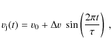
with mean velocity v0=180 km s-1 and all the combinations of half-amplitudes
![\begin{figure}
\par\includegraphics[height=17cm,angle=-90]{13908fig5.eps}\vspace*{1.3mm}
\end{figure}](/articles/aa/full_html/2010/09/aa13908-09/img50.png)
|
Figure 5:
HH 444 H |
| Open with DEXTER | |
![\begin{figure}
\par\includegraphics[height=17cm,angle=-90]{13908fig6.eps}
\end{figure}](/articles/aa/full_html/2010/09/aa13908-09/img51.png)
|
Figure 6:
HH 444 H |
| Open with DEXTER | |
The six jet models have top-hat initial cross sections with
a radius
![]() cm (corresponding to
cm (corresponding to
![]() at a distance of 450 pc), number density
at a distance of 450 pc), number density
![]() cm-3 and temperature
cm-3 and temperature
![]() K.
These parameters give a mean mass-loss rate
K.
These parameters give a mean mass-loss rate
![]() yr-1for the jet. The jet moves into a uniform environment with
density
yr-1for the jet. The jet moves into a uniform environment with
density
![]() cm-3 and temperature
cm-3 and temperature
![]() K.
K.
The time-integrations are computed with a cylindrically
symmetric version of the ``yguazú-a''
code in a 4-level, binary adaptive grid with a maximum
resolution of
![]() cm along the two axes.
A detailed description of the ``yguazú-a'' code is
given by Raga et al. (2000a).
cm along the two axes.
A detailed description of the ``yguazú-a'' code is
given by Raga et al. (2000a).
We consider that hydrogen is fully ionized throughout the computational grid, and we impose a minimum temperature of 104 K (for higher temperatures, the parametrized cooling function of Raga et al. 2000b is included). This is an approximate way of simulating a fully photoinized jet.
We note that Raga et al. (2000c) estimated that
the HH 444 flow would become fully photoionized by the
external UV radiation field at a distance of
![]() cm
from V510 Ori. Therefore, the approximation
of a fully photoionized flow is incorrect for distances
smaller than
cm
from V510 Ori. Therefore, the approximation
of a fully photoionized flow is incorrect for distances
smaller than
![]() cm from the outflow source.
cm from the outflow source.
The simulations were carried out in a
![]() cm
(axial
cm
(axial ![]() radial) cylindrical grid, with reflection conditions
on the symmetry axis and on the jet/counterjet symmetry plane and
trasmission conditions in the other grid boundaries. We
carried out 500 yr time integrations, in which the leading working surface
of the jet leaves the computational domain. At the later integration
times we see the emission from the knots close to the outflow source
(formed by the ejection velocity variability) without the contribution
from the jet's head and its extended bow shock wings.
radial) cylindrical grid, with reflection conditions
on the symmetry axis and on the jet/counterjet symmetry plane and
trasmission conditions in the other grid boundaries. We
carried out 500 yr time integrations, in which the leading working surface
of the jet leaves the computational domain. At the later integration
times we see the emission from the knots close to the outflow source
(formed by the ejection velocity variability) without the contribution
from the jet's head and its extended bow shock wings.
In the rest of the paper we assume a distance D=450 pc to the HH 444 outflow. This distance is used to scale the model predictions so that they can be directly compared with the observations.
4 The H
maps
4.1 Maps obtained from all models
We now assume that the jet axis lies at a
![]() angle
with respect to the plane of the sky (consistent with the angle
determined for HH 444 by López-Martín et al. 2001), and compute
H
angle
with respect to the plane of the sky (consistent with the angle
determined for HH 444 by López-Martín et al. 2001), and compute
H![]() maps from the t=375 yr flow stratifications obtained
from models M1-M6 (see Table 1). The maps are obtained by integrating
the H
maps from the t=375 yr flow stratifications obtained
from models M1-M6 (see Table 1). The maps are obtained by integrating
the H![]() emission coefficient (obtained from the H recombination
cascade) along lines of sight.
emission coefficient (obtained from the H recombination
cascade) along lines of sight.
The resulting maps are shown, together with the H![]() image of
HH 444, in Fig. 3. From this figure, it is evident that the models
produce a well collimated, narrow H
image of
HH 444, in Fig. 3. From this figure, it is evident that the models
produce a well collimated, narrow H![]() emitting region close
to the source and broad knots at larger distances, qualitatively
resembling the emission from the HH 444 jet base and from
the knots HH 444B and C.
emitting region close
to the source and broad knots at larger distances, qualitatively
resembling the emission from the HH 444 jet base and from
the knots HH 444B and C.
Models M1 and M2 (with a ![]() yr variability period, see Table 1)
reproduce the separation between knots B and C. However, a
well-defined H
yr variability period, see Table 1)
reproduce the separation between knots B and C. However, a
well-defined H![]() knot is seen at
knot is seen at ![]() from the source,
which does not exist in HH 444. Models M3 and M4
(with
from the source,
which does not exist in HH 444. Models M3 and M4
(with ![]() yr) have two knots, which
have a separation a factor of
yr) have two knots, which
have a separation a factor of ![]() larger than the separation
beween HH 444B and C. Finally, models M5 and M6 (with
larger than the separation
beween HH 444B and C. Finally, models M5 and M6 (with ![]() yr,
see Table 1) have a single knot at the position of HH 444C.
yr,
see Table 1) have a single knot at the position of HH 444C.
It is clear that while all models have qualitative
similarities to the observations, it appears that
the H![]() emission structure of HH 444 cannot be reproduced
by a model with a single-mode, periodic ejection variability.
In order to obtain the correct knot separations it will be
necessary to consider at least a two-mode ejection variability
model (like the one explored by Raga & Noriega-Crespo 1998),
or possibly a non-periodic ejection variability (like
the one recently explored by Yirak et al. 2009). A two-mode
ejection variability model is presented in Sect. 5.
emission structure of HH 444 cannot be reproduced
by a model with a single-mode, periodic ejection variability.
In order to obtain the correct knot separations it will be
necessary to consider at least a two-mode ejection variability
model (like the one explored by Raga & Noriega-Crespo 1998),
or possibly a non-periodic ejection variability (like
the one recently explored by Yirak et al. 2009). A two-mode
ejection variability model is presented in Sect. 5.
It is also clear that in the region close to the source
the relative H![]() emission from the jet base predicted from
all models is much stronger than that observed in HH 444.
In order to reconcile the observations and model predictions
it is therefore necessary to invoke
a relatively strong circumstellar extinction close to
V510 Ori.
emission from the jet base predicted from
all models is much stronger than that observed in HH 444.
In order to reconcile the observations and model predictions
it is therefore necessary to invoke
a relatively strong circumstellar extinction close to
V510 Ori.
4.2 The time-evolution of the H
maps
We now focus on model M4 (with ![]() yr and
yr and
![]() km s-1,
see Table 1) and compute a time-series of H
km s-1,
see Table 1) and compute a time-series of H![]() maps covering
a full ejection variability period. The resulting maps are shown
in Fig. 4.
maps covering
a full ejection variability period. The resulting maps are shown
in Fig. 4.
In this time-series, we see the formation of a knot at
![]() from the source (in the t=375 yr frame of
Fig. 4). This knot travels away from the source and
grows in angular size, and in the last two time-frames
(t=450, 475 yr) reaches the position of the HH 444B and
C knots.
from the source (in the t=375 yr frame of
Fig. 4). This knot travels away from the source and
grows in angular size, and in the last two time-frames
(t=450, 475 yr) reaches the position of the HH 444B and
C knots.
The t=475 yr frame corresponds to a full ejection
variability period after the t=375 yr frame (the last and
first frames of Fig. 4, respectively). These two H![]() maps are very similar, with the exception that
the knot at
maps are very similar, with the exception that
the knot at
![]() from the source is fainter
in the t=475 yr frame. This is because
the cocoon gas is progressively evacuated from the
computational domain, resulting in lower pre-shock densities
for the successive bow shocks travelling away from the
source.
from the source is fainter
in the t=475 yr frame. This is because
the cocoon gas is progressively evacuated from the
computational domain, resulting in lower pre-shock densities
for the successive bow shocks travelling away from the
source.
4.3 The orientation with respect to the plane of the sky
We now consider the t=375 yr frame of model M4 (see Fig. 4),
and compute H![]() maps for different angles
maps for different angles ![]() between
the outflow axis and the plane of the sky. For
between
the outflow axis and the plane of the sky. For ![]() we have a knot at
we have a knot at
![]() from the source. This knot
has a flat, bow-shaped emission structure, which does
not resemble the round morphology of the knots HH 444B and C.
from the source. This knot
has a flat, bow-shaped emission structure, which does
not resemble the round morphology of the knots HH 444B and C.
As we go to higher values of ![]() ,
the simulated knot
approaches the source and develops a rounder
morphology. For
,
the simulated knot
approaches the source and develops a rounder
morphology. For
![]() the
morphology of the simulated knot resembles the structures
of the HH 444B and C knots.
the
morphology of the simulated knot resembles the structures
of the HH 444B and C knots.
From this we conclude that the morphologies observed
for the HH 444B and C knots are consistent with the morphologies
found for the emission from internal working surfaces when
the outflow axis is at an angle
![]() with
respect to the plane of the sky. This result is consistent
with the
with
respect to the plane of the sky. This result is consistent
with the
![]() angle (between the outflow
axis and the plane of the sky) determined by López-Martín
et al. (2001) for the HH 444 outflow.
angle (between the outflow
axis and the plane of the sky) determined by López-Martín
et al. (2001) for the HH 444 outflow.
5 A two-mode ejection velocity variability model
5.1 The H
maps
The available observations of HH 444 are not sufficient to constrain a two- or three-mode ejection variability. This was possible in the past for objects in which more extensive kinematic information (i.e., of a spatially more extended region along the outflow axis) as well as proper motions are available. Examples of this are HH 34 and HH 444 (see Raga et al. 2002) and HH 30 (Anglada et al. 2007; Esquivel et al. 2007).
![\begin{figure}
\par\includegraphics[height=8cm,angle=-90,clip]{13908fig7.eps}
\end{figure}](/articles/aa/full_html/2010/09/aa13908-09/img71.png)
|
Figure 7:
H |
| Open with DEXTER | |
For this reason, we only present one two-mode ejection
velocity variability model to illustrate that
it is indeed possible to produce knot structures that
resemble the HH 444 jet. We choose a model that has a
velocity variability with two sinusoidal modes with half-amplitudes
![]() km s-1 and
km s-1 and
![]() km s-1and corresponding periods
km s-1and corresponding periods ![]() yr and
yr and
![]() km s-1. The mean velocity
v0=180 km s-1, and the remaining parameters of the
models are identical to those of models M1-M6 (see Sect. 3).
The computation is done (as in models M1-M6, see Sect. 3)
in a 4-level, binary adaptive grid with a maximum resolution
km s-1. The mean velocity
v0=180 km s-1, and the remaining parameters of the
models are identical to those of models M1-M6 (see Sect. 3).
The computation is done (as in models M1-M6, see Sect. 3)
in a 4-level, binary adaptive grid with a maximum resolution
![]() cm (along the two axes).
cm (along the two axes).
In Fig. 6 we present a comparison between the H![]() image
of HH 444 and a time-series of H
image
of HH 444 and a time-series of H![]() maps computed from
the two-mode ejection velocity variability jet model. It is clear
that a number of time-frames (e.g., the maps obtained
for t=350, 375, 425, and 600 yr) have knot distributions
that qualitatively resembles the HH 444 knot structure.
maps computed from
the two-mode ejection velocity variability jet model. It is clear
that a number of time-frames (e.g., the maps obtained
for t=350, 375, 425, and 600 yr) have knot distributions
that qualitatively resembles the HH 444 knot structure.
5.2 Convergence study
We use this two-mode jet model to illustrate the
numerical convergence of our simulations. All
results presented above were obtained using a
4-level, binary adaptive grid with a maximum resolution
![]() cm (along the two axes).
This implies that the initial jet radius (
cm (along the two axes).
This implies that the initial jet radius (
![]() cm,
see Sect. 3) is only resolved with three grid points. While the
resolution of the jet beam improves at larger distances from
the source (due to the lateral expansion of the beam), this
is indeed a rather low resolution, and one might suspect that
the results will change for higher resolutions.
cm,
see Sect. 3) is only resolved with three grid points. While the
resolution of the jet beam improves at larger distances from
the source (due to the lateral expansion of the beam), this
is indeed a rather low resolution, and one might suspect that
the results will change for higher resolutions.
In Fig. 7 we show the t=400 yr H![]() map obtained
from our two-mode jet model computed with three different
maximum resolutions:
map obtained
from our two-mode jet model computed with three different
maximum resolutions:
![]() ,
,
![]() and
and
![]() cm
(computed in binary grids with 4, 5 and 6 levels, respectively).
From this figure, it is clear that while the general morphology
of the predicted H
cm
(computed in binary grids with 4, 5 and 6 levels, respectively).
From this figure, it is clear that while the general morphology
of the predicted H![]() maps does not change with increasing
resolution of the simulation, the fluxes of the knots do
change.
maps does not change with increasing
resolution of the simulation, the fluxes of the knots do
change.
![\begin{figure}
\par\includegraphics[width=9cm,clip]{13908fig8.eps}
\end{figure}](/articles/aa/full_html/2010/09/aa13908-09/img76.png)
|
Figure 8:
Peak H |
| Open with DEXTER | |
![\begin{figure}
\par\includegraphics[width=9cm,clip]{13908fig9.eps}
\end{figure}](/articles/aa/full_html/2010/09/aa13908-09/img77.png)
|
Figure 9:
H |
| Open with DEXTER | |
This change in H![]() intensity as a function of resolution
is shown in Fig. 8, in which we plot the peak H
intensity as a function of resolution
is shown in Fig. 8, in which we plot the peak H![]() intensities of the three knots (seen in the t=400 yr
H
intensities of the three knots (seen in the t=400 yr
H![]() maps, see Fig. 7) as a function of maximum
resolution
maps, see Fig. 7) as a function of maximum
resolution ![]() of the simulations. If we look
at the brightest knot, we see that the peak H
of the simulations. If we look
at the brightest knot, we see that the peak H![]() intensity drops by a factor of
intensity drops by a factor of ![]() when going
from the
when going
from the
![]() to the
to the
![]() cm resolution. Its
peak H
cm resolution. Its
peak H![]() intensity again drops when going
from the
intensity again drops when going
from the
![]() to the
to the
![]() cm resolution, but
only by a factor of
cm resolution, but
only by a factor of ![]() .
Similar results
are found for the other two knots.
.
Similar results
are found for the other two knots.
These results indicate that at least a partial
numerical convergence is obtained for the
H![]() intensity maps when we reach our highest,
intensity maps when we reach our highest,
![]() cm resolution. We
then use this higher resolution simulation to compute
the jet width as a function of position,
with relative confidence that the results are
quantitatively meaningful. This is described in
the following section.
cm resolution. We
then use this higher resolution simulation to compute
the jet width as a function of position,
with relative confidence that the results are
quantitatively meaningful. This is described in
the following section.
5.3 Width vs. position
Let us now explore whether or not our two-mode jet model
results in a width vs. position distribution which resembles
the one observed in the HH 444 jet (see Sect. 2.2). For this
analysis we consider the t=400 yr H![]() map computed
from our higher resolution simulation (with minimum cell size
map computed
from our higher resolution simulation (with minimum cell size
![]() cm, see Sect. 5.2).
cm, see Sect. 5.2).
When applying the wavelet analysis to this synthetic image,
we obtain the width vs. position shown in Fig. 9. From this figure
we see that we obtain a region extending to ![]() from the source in which the jet width is
from the source in which the jet width is
![]() ,
basically
unresolved at the resolution of the HST images.
The first knot (at a distance of
,
basically
unresolved at the resolution of the HST images.
The first knot (at a distance of
![]() from the
source) has a width of
from the
source) has a width of
![]() ,
and the second
knot (at a distance of
,
and the second
knot (at a distance of ![]() from the
source) has a width of
from the
source) has a width of
![]() .
.
We note the interesting effect seen at ![]() from the outflow source (see Fig. 9). In this inter-knot region,
the width determined for the jet beam (from the wavelet analysis)
blows up, attaining values of several arcseconds. This is
probably because in the inter-knot regions
the spatial scale of the emission is dominated by the distance
to the neighbouring knots. These broadenings in the faint
inter-knot regions are generally obtained in width determinations
based on wavelet analyses (see Figs. 1 and 2), and a similar
effect is also obtained when fitting Gaussian functions to
the jet cross-section, provided that data with a high enough
signal-to-noise ratio are used (see Raga et al. 1991).
from the outflow source (see Fig. 9). In this inter-knot region,
the width determined for the jet beam (from the wavelet analysis)
blows up, attaining values of several arcseconds. This is
probably because in the inter-knot regions
the spatial scale of the emission is dominated by the distance
to the neighbouring knots. These broadenings in the faint
inter-knot regions are generally obtained in width determinations
based on wavelet analyses (see Figs. 1 and 2), and a similar
effect is also obtained when fitting Gaussian functions to
the jet cross-section, provided that data with a high enough
signal-to-noise ratio are used (see Raga et al. 1991).
Comparing these results with those obtained from the
H![]() map of HH 444 (see Sect. 2.2 and Fig. 1), we see that
though the positions of the knots in the simulated jet do
not coincide with those of the HH 444 knots, a general
agreement is obtained between the observed and predicted
width vs. position. Both show an unresolved jet-width
region close to the source, and widths of
map of HH 444 (see Sect. 2.2 and Fig. 1), we see that
though the positions of the knots in the simulated jet do
not coincide with those of the HH 444 knots, a general
agreement is obtained between the observed and predicted
width vs. position. Both show an unresolved jet-width
region close to the source, and widths of
![]() for
the knots.
for
the knots.
6 Conclusions
We re-analyzed the HST H![]() and red [S II] images of
HH 444 obtained by Andrews et al. (2004). We applied the non-parametric
wavelet analysis technique of Riera et al. (2003) to calculate
the width vs. position along the HH 444 jet. From this analysis we found
that the jet width is basically unresolved (in both H
and red [S II] images of
HH 444 obtained by Andrews et al. (2004). We applied the non-parametric
wavelet analysis technique of Riera et al. (2003) to calculate
the width vs. position along the HH 444 jet. From this analysis we found
that the jet width is basically unresolved (in both H![]() and [S II])
close to the source, and grows to widths of
and [S II])
close to the source, and grows to widths of
![]() in the well-defined knots B and C.
in the well-defined knots B and C.
We computed a grid of jet models with a single-mode, sinusoidal
variability for the ejection velocity, with a range of values for
the periods and amplitudes that appears to be appropriate for the knots
along HH 444 (Sect. 3). H![]() maps computed from all models
(assuming a
maps computed from all models
(assuming a
![]() angle between the outflow axis and the
plane of the sky, see Fig. 3) produce knots which qualitatively
resemble the HH 444 B and C knots. We studied the effect
of changing the angle
angle between the outflow axis and the
plane of the sky, see Fig. 3) produce knots which qualitatively
resemble the HH 444 B and C knots. We studied the effect
of changing the angle ![]() (between the outflow axis and the
plane of the sky, see Fig. 5) and found that the predicted
H
(between the outflow axis and the
plane of the sky, see Fig. 5) and found that the predicted
H![]() knots resemble the HH 444 knots only for
knots resemble the HH 444 knots only for
![]() .
This result is consistent with the
.
This result is consistent with the
![]() orientation
of the HH 444 outflow estimated by López-Martín et al. (2001).
orientation
of the HH 444 outflow estimated by López-Martín et al. (2001).
A systematic difference between the model predictions and the
observations is that the models show brighter H![]() emission close
to the outflow source (in a region within
emission close
to the outflow source (in a region within ![]() from the source,
see Figs. 3-5). This result might be consistent with the fact that
the region around
from the source,
see Figs. 3-5). This result might be consistent with the fact that
the region around ![]() Orionis shows substantial circumstellar
emission (possibly including a proplyd tail, see Andrews et al.
2004), indicating the presence of a dense, circumstellar envelope
which may be producing a substantial extinction of the jet emission.
Orionis shows substantial circumstellar
emission (possibly including a proplyd tail, see Andrews et al.
2004), indicating the presence of a dense, circumstellar envelope
which may be producing a substantial extinction of the jet emission.
However, we find that the single sinusoidal mode variability models cannot explain the knot spacings observed in HH 444. This problem can be solved by proposing a model with a two-mode sinusoidal ejection velocity variability. We illustrate this possibility by computing a two-mode jet model (Sect. 5).
We chose an H![]() map predicted from this two-mode model for
computing the jet width vs. position with the wavelet analysis
technique that we used for analyzing the HH 444 images. We find
that the jet has an unresolved region close to the source
and that the jet width grows as a function of increasing distance from
the source. A comparison between the predictions (Fig. 9) and the
HH 444 H
map predicted from this two-mode model for
computing the jet width vs. position with the wavelet analysis
technique that we used for analyzing the HH 444 images. We find
that the jet has an unresolved region close to the source
and that the jet width grows as a function of increasing distance from
the source. A comparison between the predictions (Fig. 9) and the
HH 444 H![]() observations (Fig. 1) shows a qualitatively good
agreement between the predicted and observed width vs. position.
observations (Fig. 1) shows a qualitatively good
agreement between the predicted and observed width vs. position.
To summarize, we showed that the H![]() HST image of HH 444
has knots with morphologies that agree with the predictions from
a variable ejection velocity jet (if one considers an appropriate
orientation angle between the jet axis and the plane of the sky).
The knot spacings observed in HH 444, however, require at least
a two-mode ejection velocity variability.
HST image of HH 444
has knots with morphologies that agree with the predictions from
a variable ejection velocity jet (if one considers an appropriate
orientation angle between the jet axis and the plane of the sky).
The knot spacings observed in HH 444, however, require at least
a two-mode ejection velocity variability.
The two-mode time-variability that we explored is not well constrained by the present observations, and in principle a more complex variability is probably needed. An indication of the necessity of a more complex variability are the knots at larger distances from the HH 444 source: knots G and H, at distances of 114'' and 154'' (respectively) from the source (Reipurth et al. 1998). These knots can in principle be modeled through the introduction of an extra ejection variability mode (a similar morphology in the HH 34 jet was modeled in this way by Raga & Noriega-Crespo 1998). Instead of a multi-mode variability, a non-periodic variability (see Yirak et al. 2009; Bonito et al. 2010) might be present, but the richness of inter-knot spatial scales that is to be expected from a well-sampled random variability (Raga 1992) does not seem to be present in the HH 444 jet.
AcknowledgementsThis work was supported by the CONACyT grants 61547, 101356 and 101975. The work of A.Ri. was supported by the MICINN grant AYA2008-06189-C03 and AYA2008-04211-C02-01 (co-funded with FEDER funds). We acknowledge the support of E. Palacios from the ICN-UNAM computing staff. We thank John Bally (the referee) for several helpful suggestions.
References
- Andrews, S. M., Reipurth, B., Bally, J., & Heathcote, S. R. 2004, ApJ, 606, 353 [NASA ADS] [CrossRef] [Google Scholar]
- Anglada, G., López, R., Estalella, R., et al. 2007, AJ, 133, 2799 [NASA ADS] [CrossRef] [Google Scholar]
- Bally, J., & Reipurth, B. 2001, ApJ, 546, 299 [NASA ADS] [CrossRef] [Google Scholar]
- Bally, J., Johnstone, D., Joncas, G., Reipurth, B., & Mallén-Ornelas, G. 2001, AJ, 122, 1508 [NASA ADS] [CrossRef] [Google Scholar]
- Bonito, R., Orlando, S., Peres, G., et al. 2010, A&A, 511, A42 [NASA ADS] [CrossRef] [EDP Sciences] [Google Scholar]
- Bührke, T., Mundt, R., & Ray, T. 1988, A&A, 200 99 [NASA ADS] [Google Scholar]
- Cantó, J., & Raga, A. C. 1995, MNRAS, 277, 1120 [NASA ADS] [CrossRef] [Google Scholar]
- Ciardi, A., Ampleford, D. J., Lebedev, S. V., & Stehle, C. 2008, ApJ, 678, 968 [NASA ADS] [CrossRef] [Google Scholar]
- Esquivel, A., Raga, A. C., & De Colle, F. 2007, A&A, 468, 613 [NASA ADS] [CrossRef] [EDP Sciences] [Google Scholar]
- Lim, A. J., & Raga, A. C. 1998, MNRAS, 298, 871 [NASA ADS] [CrossRef] [Google Scholar]
- López-Martín, L., Raga, A. C., López, J. A., & Meaburn, J. 2001, A&A, 371, 1118 [NASA ADS] [CrossRef] [EDP Sciences] [Google Scholar]
- Masciadri, E., & Raga, A. C. 2001, AJ, 121, 408 [NASA ADS] [CrossRef] [Google Scholar]
- Masciadri, E., Velázquez, P. F., Raga, A. C., Cantó, J., & Noriega-Crespo, A. 2002, ApJ, 573, 260 [NASA ADS] [CrossRef] [Google Scholar]
- Raga, A. C. 1992, MNRAS, 258, 301 [NASA ADS] [Google Scholar]
- Raga, A. C., & Mateo, M. 1988, AJ, 95, 543 [NASA ADS] [CrossRef] [Google Scholar]
- Raga, A. C., & Noriega-Crespo, A. 1998, AJ, 116, 2943 [NASA ADS] [CrossRef] [Google Scholar]
- Raga, A. C., Mundt, R., & Ray, T. P. 1991, A&A, 252, 733 [NASA ADS] [Google Scholar]
- Raga, A. C., Navarro-González, R., & Villagrán-Muniz, M. 2000a, RMxAA, 36, 67 [Google Scholar]
- Raga, A. C., Curiel, S., Rodríguez, L. F., & Cantó, J. 2000b, A&A, 364, 763 [NASA ADS] [Google Scholar]
- Raga, A. C., López-Martín, L., Binette, L., et al. 2000c, MNRAS, 314, 681 [NASA ADS] [CrossRef] [Google Scholar]
- Raga, A. C., Cabrit, S., Dougados, C., & Lavalley, C. 2001, A&A, 367, 959 [NASA ADS] [CrossRef] [EDP Sciences] [Google Scholar]
- Raga, A. C., Velázquez, P. F., Cantó, J., & Masciadri, E. 2002, A&A, 395, 647 [NASA ADS] [CrossRef] [EDP Sciences] [Google Scholar]
- Raga, A. C., Riera, A., Masciadri, E., et al. 2004, AJ, 127, 1081 [NASA ADS] [CrossRef] [Google Scholar]
- Reipurth, B., Bally, J., Fesen, R. A., & Devine, D. 1998, Nature, 396 [Google Scholar]
- Riera, A., Raga, A. C., Reipurth, B., et al. 2003, AJ, 126, 327 [NASA ADS] [CrossRef] [Google Scholar]
- Yirak, K., Frank, A., Cunninghan, A. J., & Mitran, S. 2009, ApJ, 695, 999 [NASA ADS] [CrossRef] [Google Scholar]
Footnotes
- ...
HLA
![[*]](/icons/foot_motif.png)
- Based on observations made with the NASA/ESA Hubble Space Telescope, and obtained from the Hubble Legacy Archive, which is a collaboration between the Space Telescope Science Institute (STScI/NASA), the Space Telescope European Coordinating Facility (ST-ECF/ESA) and the Canadian Astronomy Data Centre (CADC/NRC/CSA).
All Tables
Table 1: Grid of models.
All Figures
|
|
Figure 1:
HH 444 H |
| Open with DEXTER | |
| In the text | |
|
|
Figure 2:
HH 444 [S II] 6716+30 image ( right, see Sect. 2.1)
and characteristic width
|
| Open with DEXTER | |
| In the text | |
|
|
Figure 3:
HH 444 H |
| Open with DEXTER | |
| In the text | |
|
|
Figure 4:
HH 444 H |
| Open with DEXTER | |
| In the text | |
|
|
Figure 5:
HH 444 H |
| Open with DEXTER | |
| In the text | |
|
|
Figure 6:
HH 444 H |
| Open with DEXTER | |
| In the text | |
|
|
Figure 7:
H |
| Open with DEXTER | |
| In the text | |
|
|
Figure 8:
Peak H |
| Open with DEXTER | |
| In the text | |
|
|
Figure 9:
H |
| Open with DEXTER | |
| In the text | |
Copyright ESO 2010
Current usage metrics show cumulative count of Article Views (full-text article views including HTML views, PDF and ePub downloads, according to the available data) and Abstracts Views on Vision4Press platform.
Data correspond to usage on the plateform after 2015. The current usage metrics is available 48-96 hours after online publication and is updated daily on week days.
Initial download of the metrics may take a while.