| Issue |
A&A
Volume 517, July 2010
|
|
|---|---|---|
| Article Number | A21 | |
| Number of page(s) | 10 | |
| Section | Interstellar and circumstellar matter | |
| DOI | https://doi.org/10.1051/0004-6361/200913856 | |
| Published online | 27 July 2010 | |
Sensitivity analyses of dense cloud chemical models![[*]](/icons/foot_motif.png)
V. Wakelam1,2 - E. Herbst3 - J. Le Bourlot4 - F. Hersant1,2 - F. Selsis1,2 - S. Guilloteau1,2
1 - Université de Bordeaux, Observatoire Aquitain des Sciences de l'Univers, BP 89, 33271 Floirac Cedex, France
2 - CNRS, UMR 5804, Laboratoire d'Astrophysique de Bordeaux, BP 89, 33271 Floirac Cedex, France
3 - Departments of Physics, Astronomy, and Chemistry, The Ohio State University, Columbus, OH 43210, USA
4 - Observatoire de Paris, LUTH and Université Paris-Diderot, Place J. Janssen, 92190 Meudon, France
Received 11 December 2009 / Accepted 2 April 2010
Abstract
Context. Because of new telescopes that will dramatically
improve our knowledge of the interstellar medium, chemical models will
have to be used to simulate the chemistry of many regions with diverse
properties. To make these models more robust, it is important
to understand their sensitivity to a variety of parameters.
Aims. In this article, we report a study of the sensitivity of a
chemical model of a cold dense core, with homogeneous and
time-independent physical conditions, to variations in the
following parameters: initial chemical inventory, gas temperature and
density, cosmic-ray ionization rate, chemical reaction rate
coefficients, and elemental abundances.
Methods. We used a Monte Carlo method to randomly vary
individual parameters and groups of parameters within realistic ranges.
From the results of the parameter variations, we can quantify the
sensitivity of the model to each parameter as a function of time. Our
results can be used in principle with observations to constrain some
parameters for different cold clouds. We also attempted to use the
Monte Carlo approach with all parameters varied collectively.
Results. Within the parameter ranges studied, the most critical
parameters turn out to be the reaction rate coefficients at times up to
4 ![]() 105 yr
and elemental abundances at later times. At typical times of best
agreement with observation, models are sensitive to both of these
parameters. The models are less sensitive to other parameters such as
the gas density and temperature.
105 yr
and elemental abundances at later times. At typical times of best
agreement with observation, models are sensitive to both of these
parameters. The models are less sensitive to other parameters such as
the gas density and temperature.
Conclusions. The improvement of models will require that the
uncertainties in rate coefficients of important reactions be reduced.
As the chemistry becomes better understood and more robust,
it should be possible to use model sensitivities concerning other
parameters, such as the elemental abundances and the
cosmic ray ionization rate, to yield detailed information on
cloud properties and history. Nevertheless, at the current stage, we
cannot determine the best values of all the parameters simultaneously
based on purely observational constraints.
Key words: astrochemistry - molecular processes - ISM: abundances - ISM: molecules - ISM: individual objects: L134N - ISM: individual objects: TMC-1 (CP)
1 Introduction
Molecules are powerful observational tools for the study of the physical conditions and dynamics of star-forming regions. Each step of the formation of a stellar and planetary system is characterized by a chemical composition, which directly reflects the physical conditions of the medium and its evolutionary stage. The far-infrared space telescope Herschel and (sub)-millimeter interferometer ALMA promise to open new windows on the wealth of information found in the interstellar medium (ISM). With the improvement of observational instrument sensitivity and resolution, and the opening of new wavelength ranges, more molecules will be detected in the ISM and many molecules will be detected under a wider variety of physical conditions. The more molecules detected and the more diverse physical conditions discovered, the more complex chemical models will have to be to reproduce observations.
The results of chemical models, or simulations, depend on a number of parameters or groups of parameters often poorly constrained. In this paper, we will be concerned with the sensitivity of simple gas-phase chemical simulations of cold dense interstellar cores to these parameters. The models are based on the pseudo-time-dependent approximation, in which the chemistry evolves under fixed and homogeneous density and temperature. Homogeneous models are also referred to as 0D (zero-dimensional). Although more physically reasonable models should include the formation of cold cores from more diffuse material as the chemistry progresses, such models are rare given the lack of unanimity of how the collapse proceeds.
Among the parameters in pseudo-time-dependent/0D models determined only to a limited extent by observations or their comparisons with model results are (1) the gas kinetic temperature and density; (2) the cosmic-ray ionization rate; (3) the elemental gas-phase abundances; and (4) the initial chemical inventory. We add to these parameters the rate coefficients (5) of the many chemical reactions despite the fact that they are best determined by laboratory experiments rather than by observational constraints. We discuss the parameters in turn.
- 1.
- The gas kinetic temperature and density are usually determined by the excitation conditions of observed molecular emission lines. In addition to the uncertainties in the radiative transfer analysis of the lines, inhomogeneities of the gas may exist along the same line of sight.
- 2.
- There is no direct way to measure the cosmic-ray ionization rate
 in dense clouds. There are two different approaches to constrain .
The first one, usually used, is to determine it by comparison of
modeled and observed abundances for specific ionic species or their
ratios. Currently, there appears to be a dichotomy between diffuse
clouds, in which the high abundance of H3+ leads to a large value of ,
and dense clouds, in which the ionization conditions often lead to a value of 1-2 orders of magnitude lower (McCall et al. 2003; Indriolo et al. 2009; Caselli et al. 1998; Le Petit et al. 2004; Wootten et al. 1982).
There is some indication that the difference is simply due to the
inability of low energy cosmic rays to penetrate into the center of
dense clouds (Padovani et al. 2009). A second approach is to use the value measured in the solar system (Webber 1998; Spitzer & Tomasko 1968) and consider that
is constant in the Galaxy. However, in the solar system, the low energy
end of the cosmic ray spectrum cannot be determined directly
because of the solar wind.
in dense clouds. There are two different approaches to constrain .
The first one, usually used, is to determine it by comparison of
modeled and observed abundances for specific ionic species or their
ratios. Currently, there appears to be a dichotomy between diffuse
clouds, in which the high abundance of H3+ leads to a large value of ,
and dense clouds, in which the ionization conditions often lead to a value of 1-2 orders of magnitude lower (McCall et al. 2003; Indriolo et al. 2009; Caselli et al. 1998; Le Petit et al. 2004; Wootten et al. 1982).
There is some indication that the difference is simply due to the
inability of low energy cosmic rays to penetrate into the center of
dense clouds (Padovani et al. 2009). A second approach is to use the value measured in the solar system (Webber 1998; Spitzer & Tomasko 1968) and consider that
is constant in the Galaxy. However, in the solar system, the low energy
end of the cosmic ray spectrum cannot be determined directly
because of the solar wind. - 3.
- The computed abundances of atomic and molecular species depend on the choice of elemental abundances in the gas phase. Elements are measured in absorption in the diffuse medium (Jenkins 2004). In order to reproduce the observed gas-phase composition of dense clouds, it is often assumed that heavy atoms, including S, Si, Fe, Na and Mg, are depleted further from the gas between the diffuse (or translucent) and dense phases of a cloud life. Specifically, the initial abundances of these elements in pseudo-time-dependent models are taken to be 2 to 3 orders of magnitude lower than in diffuse clouds but the efficiency of the depletions onto the grains is quite uncertain (Graedel et al. 1982). Moreover, the depletions of the elements may depend on the depth into the molecular cloud.
- 4.
- Since the t=0 time of pseudo-time-dependent models is artificial, the initial chemical inventory chosen can be artificial as well. Chemical models usually start with all the elements in the atomic form, except for H2, assuming that the density of the gas had suddenly increased from a diffuse to a dense medium. Shock models of the conversion of diffuse to dense gas show, on the other hand, that the process is slow and that a significant amount of CO may be synthesized before a sizable dense cloud core is produced (Bergin et al. 2004). Preliminary results show that the formation of complex molecules is far slower if the starting form of carbon is CO (Hassel et al. 2010). Thus, the initial chemical abundances and the cloud age, as determined by comparison of observational and model abundances, are correlated.
- 5.
- Finally, the chemistry in the dense ISM involves thousands of gas-phase reactions, especially when one is dealing with complex molecules. Only a small fraction of these reactions have been studied at the low temperatures present in cold dense cores. Thus, even for systems studied in the laboratory at higher temperatures, there can be a difficulty in extrapolating results to significantly lower temperatures. The most important reactions at assorted cloud ages have been discussed in previous papers with our sensitivity approach and those of others (Vasyunin et al. 2004; Wakelam et al. 2005,2006; Vasyunin et al. 2008).
2 Chemical model
We used a new version of the Nahoon gas-phase chemical code (Wakelam et al. 2005),
which is significantly faster than the previous version. The code is
written in Fortran 90 and the differential equation solver is
DLSODES from the ODEPACK package (http://www.netlib.org/odepack/opkd-sum).
Although the code is written for 1D models (models that can be
heterogeneous in one dimension), we used it in 0D with gas temperature
and total hydrogen density set at the standard values for cold dense
cores of T = 10 K and ![]() = 2
= 2 ![]() 104 cm-3.
The visual extinction is set to 10 so that photo-chemistry with
external UV photons is of little importance. The cosmic-ray
ionization rate
104 cm-3.
The visual extinction is set to 10 so that photo-chemistry with
external UV photons is of little importance. The cosmic-ray
ionization rate
![]() is 1.3
is 1.3 ![]() 10-17 s-1. We used the osu.03.2008 chemical network (http://www.physics.ohio-state.edu/ eric/research.html),
which contains 13 elements, 455 species, and
4508 gas-phase reactions. This particular version of the osu
network does not contain molecular anions, nor any dynamic
depletion of gas-phase species. No reactions on grains are
considered except for the production of H2 from two
H atoms, a process that is treated in a pseudo-gas-phase
manner by relating the density of grains to the overall gas density.
The osu.03.2008 chemical network used in this work is available at
the CDS with the following format. The first seven columns contain the
reactants (three columns) and the products (four columns) of
the reactions. The next three columns (
10-17 s-1. We used the osu.03.2008 chemical network (http://www.physics.ohio-state.edu/ eric/research.html),
which contains 13 elements, 455 species, and
4508 gas-phase reactions. This particular version of the osu
network does not contain molecular anions, nor any dynamic
depletion of gas-phase species. No reactions on grains are
considered except for the production of H2 from two
H atoms, a process that is treated in a pseudo-gas-phase
manner by relating the density of grains to the overall gas density.
The osu.03.2008 chemical network used in this work is available at
the CDS with the following format. The first seven columns contain the
reactants (three columns) and the products (four columns) of
the reactions. The next three columns (![]() ,
, ![]() and
and ![]() )
give the parameters to compute the rate coefficients. Column 11
indicates the type of reaction. Column 12 is the number of the
reaction within a given type of reaction whereas column 13 is the
general number of the reaction in the network. Finally, the last
column gives the uncertainty factor for the rate coefficient. More
details about the format can be found at http://www.physics.ohio-state.edu/ eric. Species are initially all in the atomic form except for H, which is 100% in H2. Table 1 summarizes our standard model.
)
give the parameters to compute the rate coefficients. Column 11
indicates the type of reaction. Column 12 is the number of the
reaction within a given type of reaction whereas column 13 is the
general number of the reaction in the network. Finally, the last
column gives the uncertainty factor for the rate coefficient. More
details about the format can be found at http://www.physics.ohio-state.edu/ eric. Species are initially all in the atomic form except for H, which is 100% in H2. Table 1 summarizes our standard model.
Listed in Table 2, the base elemental abundances used are oxygen-rich, and represent a low-sulfur version of the set labeled EA3 by Wakelam & Herbst (2008). In this set of abundances, the amount of helium is based on the observed value in the Orion Nebula (Osterbrock et al. 1992).
The oxygen, nitrogen and carbon abundances seem to be rather
constant in diffuse clouds and we have taken the values observed in ![]() Oph (Meyer et al. 1998; Cardelli et al. 1993).
Since we do not include gas depletion in Nahoon, we then
removed 2.4% of C and 13% of O to account for the
fraction depleted on grain mantles in the form of CO and H2O, as suggested by Shalabiea & Greenberg (1995). For Na+, Cl+ and P+, we use the observed values in
Oph (Meyer et al. 1998; Cardelli et al. 1993).
Since we do not include gas depletion in Nahoon, we then
removed 2.4% of C and 13% of O to account for the
fraction depleted on grain mantles in the form of CO and H2O, as suggested by Shalabiea & Greenberg (1995). For Na+, Cl+ and P+, we use the observed values in ![]() Oph (Savage & Sembach 1996).
In dense clouds, iron, silicon and magnesium show additional
depletion compared to the diffuse clouds, and we adopted the depleted
values recommended by Flower & Pineau des Forêts (2003). Sulphur is the most problematic element (see for instance Ruffle et al. 1999). The low value, taken from Graedel et al. (1982),
is the standard ``low-metal'' abundance. In summary,
our low-sulfur EA3 abundances contain probable elemental
abundances based on observational constraints. One of the consequences
is that we do not produce large abundances of complex molecules since
the C/O ratio is significantly less than unity. These base
abundances will be varied to determine the sensitivity of the model to
elemental abundances.
Oph (Savage & Sembach 1996).
In dense clouds, iron, silicon and magnesium show additional
depletion compared to the diffuse clouds, and we adopted the depleted
values recommended by Flower & Pineau des Forêts (2003). Sulphur is the most problematic element (see for instance Ruffle et al. 1999). The low value, taken from Graedel et al. (1982),
is the standard ``low-metal'' abundance. In summary,
our low-sulfur EA3 abundances contain probable elemental
abundances based on observational constraints. One of the consequences
is that we do not produce large abundances of complex molecules since
the C/O ratio is significantly less than unity. These base
abundances will be varied to determine the sensitivity of the model to
elemental abundances.
Table 1: Standard dense cloud model.
Table 2: Elemental abundances with respect to total hydrogen nuclei.
3 Sensitivity analyses
3.1 Variations for most parameters
The major goal of this analysis is to quantify the sensitivity of
chemical models to variations of the parameters within realistic ranges
of values. The method consists in generating new sets of
parameters (![]() )
using random functions and computing the corresponding chemical fractional abundances vs. time (
)
using random functions and computing the corresponding chemical fractional abundances vs. time (
![]() ).
Using such an approach, we studied the sensitivities to the reaction
rate coefficients, the gas temperature and density,
the elemental abundances, and the cosmic-ray ionization rate. The
variational range for each parameter is given in Table 3.
For the reaction rate coefficients, we have assumed an amplitude
variation equal to their uncertainties, as originally included in
the UMIST database (see http://www.udfa.net/) and subsequently in the osu database, with a log-normal distribution (see Wakelam et al. 2005,2006). We define Fi, the uncertainty factor of the rate coefficient, at a 1
).
Using such an approach, we studied the sensitivities to the reaction
rate coefficients, the gas temperature and density,
the elemental abundances, and the cosmic-ray ionization rate. The
variational range for each parameter is given in Table 3.
For the reaction rate coefficients, we have assumed an amplitude
variation equal to their uncertainties, as originally included in
the UMIST database (see http://www.udfa.net/) and subsequently in the osu database, with a log-normal distribution (see Wakelam et al. 2005,2006). We define Fi, the uncertainty factor of the rate coefficient, at a 1![]() level
of confidence. As a consequence, there is a 68.3%
chance that the rate coefficient lies between
ki/Fi and ki
level
of confidence. As a consequence, there is a 68.3%
chance that the rate coefficient lies between
ki/Fi and ki ![]() Fi, where ki is the listed rate coefficient for reaction i.
For the other parameters, except for the initial chemical
inventory (see below), flat distributions (no preferred values)
were assumed with ranges determined by reasonable uncertainties, which
are mainly
Fi, where ki is the listed rate coefficient for reaction i.
For the other parameters, except for the initial chemical
inventory (see below), flat distributions (no preferred values)
were assumed with ranges determined by reasonable uncertainties, which
are mainly ![]() 50%
from the center or peak value. The gas temperature then lies
between 5 and 15 K, the total hydrogen density between
1
50%
from the center or peak value. The gas temperature then lies
between 5 and 15 K, the total hydrogen density between
1 ![]() 104 and 3
104 and 3 ![]() 104 cm-3, and the elemental abundances between
104 cm-3, and the elemental abundances between ![]() 50%
of their standard values. The cosmic ray ionization rate,
which is clearly uncertain to more than a factor of two, is varied
between 5
50%
of their standard values. The cosmic ray ionization rate,
which is clearly uncertain to more than a factor of two, is varied
between 5 ![]() 10-18 and 5
10-18 and 5 ![]() 10-17 s-1.
10-17 s-1.
Table 3: Variational ranges of the parameters.
The variations of the elemental abundances are sufficient to probe perturbations around the chosen values, including C/O ratios greater than unity, but not large enough to include the total diversity used by previous modelers. All individual parameters (e.g., the cosmic ray ionization rate) or groups of parameters (e.g., reaction rate coefficients, elemental abundances) were varied one at a time except for the temperature and the density, which were varied together although they are not correlated. In total, we ran 8000 different models of the dense cloud in varying these parameters. We used a Monte Carlo method to sample parameters randomly; this is most efficient for groups of parameters such as the reaction rate coefficients. For individual parameters such as the cosmic-ray ionization rate, a non-random sampling method could have been used to span the range of values.
To quantify the dispersion of the computed abundance profile of a
specific species at a given time when one parameter or a number of
different parameters is varied, we calculate the standard deviation of
the profile in logarithmic units using the formula
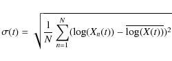
|
(1) |
where the sum is over the number of computed abundances N, Xn(t) is the abundance of the specific species for run n at time t and
3.2 Determination of the initial chemical inventory
The initial atomic and molecular abundances for the cold core are
treated uniquely. To study the sensitivity to the initial
concentrations, we need to have realistic distributions for dense cloud
models. Since dense molecular clouds are presumably formed from diffuse
or translucent gas, we first compute the steady-state chemical
composition of such a gas with a temperature of 50 K, a total
hydrogen density of 2 ![]() 103 cm-3
and a visual extinction of unity. The species start in their atomic
form prior to the diffuse/translucent cloud stage, except for hydrogen,
which is assumed to be divided equally among atomic and molecular
forms. The fixed elemental abundances used for the diffuse/translucent
stage are the ones listed in Table 2,
although a more realistic set would have less depletion. In order
to get realistic distributions, we randomly varied the reaction rate
coefficients within their uncertainty ranges using an additional
3500 runs. The abundances and distributions we obtained at
steady-state were then used as the initial chemical inventory for the
dense cloud. As an example, the CO abundance
distribution in the diffuse/translucent cloud conditions is shown in
Fig. 1 (upper and middle panels) as a function of time. The distribution of CO at steady-state (107 yr)
used as the initial distribution for the dense cloud is shown on the
lower panel and can be fitted by a log-normal distribution.
It peaks at a fractional abundance of
103 cm-3
and a visual extinction of unity. The species start in their atomic
form prior to the diffuse/translucent cloud stage, except for hydrogen,
which is assumed to be divided equally among atomic and molecular
forms. The fixed elemental abundances used for the diffuse/translucent
stage are the ones listed in Table 2,
although a more realistic set would have less depletion. In order
to get realistic distributions, we randomly varied the reaction rate
coefficients within their uncertainty ranges using an additional
3500 runs. The abundances and distributions we obtained at
steady-state were then used as the initial chemical inventory for the
dense cloud. As an example, the CO abundance
distribution in the diffuse/translucent cloud conditions is shown in
Fig. 1 (upper and middle panels) as a function of time. The distribution of CO at steady-state (107 yr)
used as the initial distribution for the dense cloud is shown on the
lower panel and can be fitted by a log-normal distribution.
It peaks at a fractional abundance of
![]()
![]() 10-5 with a standard deviation of a factor of 6.3. For comparison, the C+ and C distributions have their steady-state peaks at
10-5 with a standard deviation of a factor of 6.3. For comparison, the C+ and C distributions have their steady-state peaks at
![]()
![]() 10-5 and
10-5 and
![]() respectively, so that the gas is still mainly atomic except for H2, which takes up most of the elemental hydrogen; the atomic H distribution peaks at
respectively, so that the gas is still mainly atomic except for H2, which takes up most of the elemental hydrogen; the atomic H distribution peaks at
![]()
![]() 10-3.
These results are somewhat different from our typical assumption that
carbon and oxygen are purely atomic and hydrogen purely molecular at
the initial stage of a dense cloud. Our distributions span two
extreme scenarios: one in which most of the carbon is still in the
atomic form (C+ abundance
10-3.
These results are somewhat different from our typical assumption that
carbon and oxygen are purely atomic and hydrogen purely molecular at
the initial stage of a dense cloud. Our distributions span two
extreme scenarios: one in which most of the carbon is still in the
atomic form (C+ abundance
![]()
![]() 10-4) and one in which CO is the dominant form of carbon (CO abundance
10-4) and one in which CO is the dominant form of carbon (CO abundance
![]()
![]() 10-4). These extreme values can arise depending upon parameters in the shock models for dense cloud formation of Bergin et al. (2004).
10-4). These extreme values can arise depending upon parameters in the shock models for dense cloud formation of Bergin et al. (2004).
![\begin{figure}
\par\includegraphics[width=8cm,clip]{13856fg1.eps}
\end{figure}](/articles/aa/full_html/2010/09/aa13856-09/img34.png)
|
Figure 1:
CO abundance computed in a diffuse/translucent cloud. Upper panel: plot of 10% of the runs. Middle panel:
the gray levels represents the percentage of runs. Any level
of gray: at least one run. Two darkest gray levels: 95% of
all runs at one given time (2 sigma if the distribution is
log-normal). Darkest gray: 68% of all runs (1 sigma if the
distribution is log-normal). Lower panel: distribution of the fractional abundance at 107 yr, where the median value is approximately 2 |
| Open with DEXTER | |
3.3 Variation of all parameters
In the sections presented above, we have emphasized how we vary the parameters or groups of parameters one after the other to study their effect independently. The alternative approach is to develop a model in which all parameters are varied collectively. To achieve this goal, we have once again used a two-step procedure involving the diffuse and dense cloud stages, discussed below. The procedure is also summarized in Fig. 2 for better understanding.
For the first step, we once again compute the steady-state chemical
composition of a diffuse cloud with a fixed temperature of 50 K,
a density of 2 ![]() 103 cm-3, visual extinction of unity, and cosmic-ray ionization rate of 1.3
103 cm-3, visual extinction of unity, and cosmic-ray ionization rate of 1.3 ![]() 10-17 s-1
(as described in the previous subsection). But now we vary at
the same time the elemental abundances and the rate coefficients within
the ranges given in Sect. 3.1, using the Monte-Carlo approach with a different distribution of random numbers for both sets of parameters. We obtain N=3500 different
steady-state chemical compositions as a consequence of varying the sets
of elemental abundances and rate coefficients simultaneously.
In the second step, we use this distribution of 3500 chemical
compositions as the initial inventory and compute the chemical
evolution of a dense cloud using the previous 3500 sets of rate
coefficients. In addition, we vary simultaneously the temperature,
the density and the cosmic-ray ionization rate using different
random number distributions for each parameter. We then obtain
3500 different chemical evolutionary paths, each of which
corresponds to to a different temperature, density, cosmic-ray
ionization rate, set of rate coefficients, set of elemental
abundances and initial chemical composition.
10-17 s-1
(as described in the previous subsection). But now we vary at
the same time the elemental abundances and the rate coefficients within
the ranges given in Sect. 3.1, using the Monte-Carlo approach with a different distribution of random numbers for both sets of parameters. We obtain N=3500 different
steady-state chemical compositions as a consequence of varying the sets
of elemental abundances and rate coefficients simultaneously.
In the second step, we use this distribution of 3500 chemical
compositions as the initial inventory and compute the chemical
evolution of a dense cloud using the previous 3500 sets of rate
coefficients. In addition, we vary simultaneously the temperature,
the density and the cosmic-ray ionization rate using different
random number distributions for each parameter. We then obtain
3500 different chemical evolutionary paths, each of which
corresponds to to a different temperature, density, cosmic-ray
ionization rate, set of rate coefficients, set of elemental
abundances and initial chemical composition.
4 Results
In Sects. 4.1-4.4 below, we discuss the sensitivities of the abundances to individual variations of parameters or groups of parameters with the others set equal to their standard values. Afterwards we compare these sensitivities and also consider the sensitivities to all parameters varied collectively.
| Figure 2: Steps used to vary all the parameters of the model collectively. |
|
| Open with DEXTER | |
4.1 Sensitivity to the initial concentrations and their distributions
![\begin{figure}
\par\includegraphics[width=8.8cm,clip]{13856fg3.eps}
\end{figure}](/articles/aa/full_html/2010/09/aa13856-09/img36.png)
|
Figure 3: O2, CH, C3O and HC7N abundances as a function of time in the dense cloud stage, starting with a distribution of atomic and molecular abundances discussed in the text. The black lines represent abundances obtained if we use our standard atomic initial concentrations except for H2. |
| Open with DEXTER | |
The sensitivities of selected dense cloud abundances to changes in initial chemical concentrations are shown in Fig. 3
as functions of time. The initial distributions of the molecular
concentrations introduce spreads in the time-dependent solutions that
last until the system is at steady state, where abundances no longer
depend on the initial concentrations because we do not have any
bistability for the parameters used. Although some distributions,
such as that for atomic H, show standard deviations (
![]() ,
see Sect. 3.1) as large as a factor of
,
see Sect. 3.1) as large as a factor of
![]() for times in the dense cloud stage up to 105 yr, most distributions are more sharply peaked, as can be seen in Fig. 3. For the species shown in this figure, the actual logarithmic standard deviations
for times in the dense cloud stage up to 105 yr, most distributions are more sharply peaked, as can be seen in Fig. 3. For the species shown in this figure, the actual logarithmic standard deviations ![]() for O2, CH, C3O and HC7N are 0.14, 0.12, 0.07 and 0.17 respectively at 105 yr.
For comparison, we have started the dense cloud stage with our
standard initial chemical abundances - atoms except for 100% H2 - at the elemental abundances found in Table 2. The fractional abundances obtained with these initial concentrations are also plotted in Fig. 3
with single black lines. For most molecules, there is very
little difference between the black lines and the distributions at any
time, although what differences exist occur mainly at earlier times.
For complex molecules however, such as HC7N, CH3OH, and NH2CHO, which typically peak at so-called early times in the range 104-6 yr,
the early-time abundances are significantly higher with the
standard than with the calculated initial abundances.
for O2, CH, C3O and HC7N are 0.14, 0.12, 0.07 and 0.17 respectively at 105 yr.
For comparison, we have started the dense cloud stage with our
standard initial chemical abundances - atoms except for 100% H2 - at the elemental abundances found in Table 2. The fractional abundances obtained with these initial concentrations are also plotted in Fig. 3
with single black lines. For most molecules, there is very
little difference between the black lines and the distributions at any
time, although what differences exist occur mainly at earlier times.
For complex molecules however, such as HC7N, CH3OH, and NH2CHO, which typically peak at so-called early times in the range 104-6 yr,
the early-time abundances are significantly higher with the
standard than with the calculated initial abundances.
One reason may lie in the relatively high abundance of atomic hydrogen
calculated at steady-state in the diffuse stage. Unlike the case for
standard abundances, in which, starting from zero,
the fractional abundance of atomic H reaches a
constant 10-4 by 103 yr, the calculated atomic hydrogen distribution at steady-state in the diffuse stage remains peaked at
![]()
![]() 10-3 for up to 105 yr in the dense cloud stage. Note that our model includes the H2 and CO self-shielding using approximations from Lee et al. (1996).
The excess atomic hydrogen calculated in the diffuse cloud stage
and used initially in the dense cloud stage can interfere with the
production of complex molecules by depleting some intermediate
hydrocarbon radicals via neutral-neutral reactions. Another possible
reason is the relatively high abundance of CO calculated to occur at
steady-state in the diffuse stage. Once a significant amount of carbon
becomes entrained in CO, it is not as easy to form complex
carbon-containing species.
10-3 for up to 105 yr in the dense cloud stage. Note that our model includes the H2 and CO self-shielding using approximations from Lee et al. (1996).
The excess atomic hydrogen calculated in the diffuse cloud stage
and used initially in the dense cloud stage can interfere with the
production of complex molecules by depleting some intermediate
hydrocarbon radicals via neutral-neutral reactions. Another possible
reason is the relatively high abundance of CO calculated to occur at
steady-state in the diffuse stage. Once a significant amount of carbon
becomes entrained in CO, it is not as easy to form complex
carbon-containing species.
| Figure 4: Left panel: calculated HC3N, C5H and CH3OH abundances as a function of the initial concentration ratio C+/CO of the dense cloud stage. Right panel: calculated CH2 and HC3N abundances as a function of initial atomic hydrogen fractional abundance. Results are shown for 105 yr. |
|
| Open with DEXTER | |
To determine which of these effects is the more important for the dense cloud stage, we first varied the initial C+/CO dense cloud ratio over a wide range while fixing the overall carbon abundance as well as the other elemental abundances at the standard values shown in Table 2. We separately did an analogous variation for the initial H/H2 ratio in the dense cloud stage, in which case all the carbon lies initially in C+. Some results at a dense cloud time of 105 yr can be seen in Fig. 4. Larger carbon-containing organic species are clearly enhanced for larger initial C+/CO ratios, but there is a saturation point for C+/CO larger than 1. Because our standard initial C+/CO ratio exceeds unity and our calculated dense cloud initial abundance ratio has a median value near 5, the variation of this ratio between our two sets of initial concentrations is not the reason for differences in abundances of complex molecules such as HC7N. Regarding the initial fractional abundance of atomic hydrogen, however, we see that even the smaller organic species CH2 and HC3N are reduced in abundance as the ratio increases to 10-3; the reduction in abundance shown is even larger for more complex species. Note that there is also a saturation effect here. In particular, the molecular abundances are not sensitive to H initial abundances smaller than 10-5, but this value is well below the range of values in our calculations. Within the ranges of initial concentrations for the dense cloud stage studied, the major source of sensitivity is thus the residual atomic hydrogen abundance. For initial concentrations, however, in which there is more CO than C+, the abundances of larger organic species will be significantly reduced at early times. The fact that a large abundance of atomic hydrogen can significantly reduce calculated peak abundances of complex molecules at early time is of some importance considering that 21 cm absorption studies indicate significant abundances of atomic H in some cold cores that are higher than calculated by our standard model (Krco et al. 2009). This possible discrepancy argues against the high calculated early-time abundances for complex molecules in the simple pseudo-time-dependent model and for its possible replacement by models that take into account cloud formation and heterogeneity. On the other hand, the presence of anions or PAH's, not included in this study, tends to aid the synthesis of complex molecules (Walsh et al. 2009; Wakelam & Herbst 2008).
In the variations of the other parameters discussed below, we return to our standard initial chemical abundances for dense clouds. This choice maximizes complex molecule abundances at early times. Nevertheless, the abundances achieved are still low compared with low-metal elemental abundances, as can be seen in the recent calculations of Walsh et al. (2009).
4.2 Sensitivity to the reaction rate coefficients, temperature, and density
The sensitivities of atomic and molecular abundances in cold dense
clouds to variations in reaction rate coefficients and gas temperature
and density have already been studied by Wakelam et al. (2006).
For this reason, we will just mention the salient results of our
new calculations. For rate coefficients, the computed abundances
have log-normal distributions resulting from the probability
distribution functions of the reaction rate coefficients (see Wakelam et al. 2006).
Moreover, a variation of temperature within the range 5-15 K
mainly affects the nitrogen-bearing species. In fact, much of
the nitrogen chemistry starts with the reaction N+ + H2
![]() NH+ + H,
which is either slightly endothermic or possesses a small barrier. The
rate coefficient of this reaction at temperatures under 100 K
depends upon the fraction of molecular hydrogen in its excited ortho
state; the results of more detailed calculations (Le Bourlot 1991)
yield an effective activation energy of 85 K for the
temperature range 10-100 K, as listed in the osu network.
Temperatures below 10 K then produce smaller abundances of
N-bearing species than temperatures above 10 K (see Fig. 4 of Wakelam et al. 2006). Within the chosen range, the density has little influence on the abundances.
NH+ + H,
which is either slightly endothermic or possesses a small barrier. The
rate coefficient of this reaction at temperatures under 100 K
depends upon the fraction of molecular hydrogen in its excited ortho
state; the results of more detailed calculations (Le Bourlot 1991)
yield an effective activation energy of 85 K for the
temperature range 10-100 K, as listed in the osu network.
Temperatures below 10 K then produce smaller abundances of
N-bearing species than temperatures above 10 K (see Fig. 4 of Wakelam et al. 2006). Within the chosen range, the density has little influence on the abundances.
4.3 Sensitivity to the cosmic-ray ionization rate
Most of the molecules are sensitive to the cosmic-ray ionization rate (![]() )
since cosmic ray ionization is the main source of atomic and
molecular ions for cold clouds, and the abundances of neutral
species are determined mainly by reactions involving ions and/or
electrons. Sensitive species can be divided into two groups:
1) those sensitive to a change in
)
since cosmic ray ionization is the main source of atomic and
molecular ions for cold clouds, and the abundances of neutral
species are determined mainly by reactions involving ions and/or
electrons. Sensitive species can be divided into two groups:
1) those sensitive to a change in ![]() at all times and 2) those only sensitive to
at all times and 2) those only sensitive to ![]() between 104 and 107 yr. The first group is composed of molecules that are more or less direct products of the ionization of H2 by cosmic rays, such as H3+, OH (see Fig. 5) and O2. Complex molecules, such as the cyanopolyynes, are part of the second group, as can be seen in Fig. 6 for the case of HC3N. Some molecular abundances increase as
between 104 and 107 yr. The first group is composed of molecules that are more or less direct products of the ionization of H2 by cosmic rays, such as H3+, OH (see Fig. 5) and O2. Complex molecules, such as the cyanopolyynes, are part of the second group, as can be seen in Fig. 6 for the case of HC3N. Some molecular abundances increase as ![]() increases (for instance OH, CO, O2, C3, C3O, SO, NO, and most of the ions), whereas others clearly decrease with increasing
increases (for instance OH, CO, O2, C3, C3O, SO, NO, and most of the ions), whereas others clearly decrease with increasing ![]() (for instance the cyanopolyynes, H2O, OCS, CS, CH3OH and HCN). The cases of OH and HC3N can be seen in the right panels of Figs. 5 and 6.
Presumably, the distinction for neutral species arises from
whether or not ions are more important in the formation or the
destruction of molecular species. The species OH and H2O for instance are both produced by the dissociative recombination of H3O+ but H2O is mainly destroyed by an ion-molecular reaction with C+ whereas OH is destroyed by reaction with neutral N.
(for instance the cyanopolyynes, H2O, OCS, CS, CH3OH and HCN). The cases of OH and HC3N can be seen in the right panels of Figs. 5 and 6.
Presumably, the distinction for neutral species arises from
whether or not ions are more important in the formation or the
destruction of molecular species. The species OH and H2O for instance are both produced by the dissociative recombination of H3O+ but H2O is mainly destroyed by an ion-molecular reaction with C+ whereas OH is destroyed by reaction with neutral N.
| Figure 5:
OH sensitivity to the cosmic-ray ionization rate ( |
|
| Open with DEXTER | |
| Figure 6:
HC3N sensitivity to the cosmic-ray ionization rate ( |
|
| Open with DEXTER | |
The dependence on ![]() at steady state has been discussed previously by Lepp & Dalgarno (1996) and Lee et al. (1998), who found that when photodestruction by external photons is ignorable, then fractional abundances depend on the ratio
at steady state has been discussed previously by Lepp & Dalgarno (1996) and Lee et al. (1998), who found that when photodestruction by external photons is ignorable, then fractional abundances depend on the ratio
![]() .
Thus the fact that the distribution for HC3N collapses to near a point at steady state despite the large variation in
.
Thus the fact that the distribution for HC3N collapses to near a point at steady state despite the large variation in ![]() shows that there is also very little dependence on
shows that there is also very little dependence on ![]() whereas the distribution for OH shows that this radical has some (inverse) dependence on
whereas the distribution for OH shows that this radical has some (inverse) dependence on ![]() .
.
4.4 Sensitivity to the elemental abundances
![\begin{figure}
\par\includegraphics[width=8.8cm,clip]{13856fg8.eps}
\end{figure}](/articles/aa/full_html/2010/09/aa13856-09/img43.png)
|
Figure 7: HC3N sensitivity to elemental abundances. Left panel: HC3N probability density as a function of time. Right upper panel: distribution of HC3N abundance at 107 yr. Right lower panel: HC3N abundance as a function of elemental C/O ratio at 107 yr. |
| Open with DEXTER | |
The effects of variations in the elemental abundances are shown in Fig. 7 for HC3N, where the distribution spreads out with increasing time, reaching a standard deviation that exceeds 1.0, which implies a 68% chance of finding the abundance to be spread over 2.5 orders of magnitude, when steady-state is finally reached. The most important variations in the range considered are those for the elements carbon and oxygen, and most of the sensitivity is to the ratio of these elements, which varies between 0.2 and 1.4. The correlation between the HC3N abundance at 107 yr and the C/O elemental ratio is shown in the right lower panel of the figure, where it can be seen that HC3N increases in abundance quite dramatically with C/O whereas the spread at a given C/O ratio caused by different values of C and O as well as variations of the other elemental abundances is smaller. In general, larger abundances of C-rich molecules such as HC3N are obtained with increasing C/O. The reason is that the greater the C/O ratio, the greater the amount of carbon that is not taken up in the form of CO. When the C/O elemental ratio becomes larger than 1, we go from a chemical regime dominated by oxygen to a regime where carbon chemistry is the more important. Since it takes some time for a large amount of CO to be synthesized, the largest effect is seen at the longest times.
4.5 Comparison of the different sensitivities
![\begin{figure}
\par\includegraphics[width=8.8cm,clip]{13856fg9.eps}
\end{figure}](/articles/aa/full_html/2010/09/aa13856-09/img44.png)
|
Figure 8:
Logarithmic standard deviations for different parameters
|
| Open with DEXTER | |
To compare the effect of each parameter, including the initial concentrations as described in Sect. 4.1, we computed the logarithmic standard deviation
![]() of the abundance distributions at each time for each parameter group i -
initial concentrations, elemental abundances, cosmic-ray ionization
rate, temperature/density, and reaction rate coefficients -
as well as for the case where we vary all parameters together.
Note again that a logarithmic standard deviation of 1.0 refers to
a factor of 10 in either direction (see Sect. 3.1).
As an illustration, we show the individual logarithmic standard
deviations for several molecules as a function of time in Fig. 8. Different molecules are sensitive to different parameters and this sensitivity varies with time. For HC3N,
the reaction rate coefficients dominate until late times when the
species is more sensitive to the elemental abundances
(see Sect. 4.4). The species NH3, on the other hand, is more sensitive to the gas temperature and density for times larger than 105 yr (see Sect. 4.2).
As expected, the standard deviation when varying all
parameters is generally larger than the ones for individual parameters
but much smaller than the sum of the individual effects.
of the abundance distributions at each time for each parameter group i -
initial concentrations, elemental abundances, cosmic-ray ionization
rate, temperature/density, and reaction rate coefficients -
as well as for the case where we vary all parameters together.
Note again that a logarithmic standard deviation of 1.0 refers to
a factor of 10 in either direction (see Sect. 3.1).
As an illustration, we show the individual logarithmic standard
deviations for several molecules as a function of time in Fig. 8. Different molecules are sensitive to different parameters and this sensitivity varies with time. For HC3N,
the reaction rate coefficients dominate until late times when the
species is more sensitive to the elemental abundances
(see Sect. 4.4). The species NH3, on the other hand, is more sensitive to the gas temperature and density for times larger than 105 yr (see Sect. 4.2).
As expected, the standard deviation when varying all
parameters is generally larger than the ones for individual parameters
but much smaller than the sum of the individual effects.
![\begin{figure}
\par\includegraphics[width=8.8cm,clip]{13856fg10.eps}
\end{figure}](/articles/aa/full_html/2010/09/aa13856-09/img45.png)
|
Figure 9:
Abundance of HC3N as a function of time for the case of all parameters varied together on the left and for the variation of rate coefficient only on the right. In each panel, the middle curve represents the median abundance while the two external curves represent a 1 |
| Open with DEXTER | |
In some cases, however, the standard deviation for all parameters is
smaller than for one of the individual parameters or parameter groups,
such as the rate-coefficient (``R.C.'') case for HC3N between 103 and 105 yr.
This situation can happen because the amplification of the error
affecting the rate coefficients and its propagation into a spread of
abundances depends on the set of parameters other than the rate
coefficients. In some cases, the standard set of parameters
will produce a dispersion that is larger than what is obtained with
most of the other sets that are generated in the case for all
parameters. As a consequence, the value of ![]() obtained by varying only the rate coefficients can be higher than what
is found when varying all the parameters together, which attenuates the
dispersion of abundances. Large values of
obtained by varying only the rate coefficients can be higher than what
is found when varying all the parameters together, which attenuates the
dispersion of abundances. Large values of ![]() are often associated with a stiff variation of the abundance, because
one of the effects of changing the rate coefficients is to produce a
time shifting of the chemical evolution. If a species
experiences a stiff variation of its abundance at a time t, this time-shifting produced by varying the rate coefficients results in a large dispersion of its abundances at t.
When the standard set of parameters produces the stiffest variation,
the deviation in the R.C. case can exceed that for all of the
parameters. In Fig. 9, we show the mean abundance of HC3N with its
are often associated with a stiff variation of the abundance, because
one of the effects of changing the rate coefficients is to produce a
time shifting of the chemical evolution. If a species
experiences a stiff variation of its abundance at a time t, this time-shifting produced by varying the rate coefficients results in a large dispersion of its abundances at t.
When the standard set of parameters produces the stiffest variation,
the deviation in the R.C. case can exceed that for all of the
parameters. In Fig. 9, we show the mean abundance of HC3N with its ![]() standard deviation in the case of the variation of all parameters and
in the case of the variation of the rate coefficients only.
For each case, we show the standard deviation obtained at 104 yr by a gray vertical line. In the R.C. case, the abundance of HC3N
increases much more stiffly than in the case for all parameters and
this introduces a larger standard deviation at a specific time.
In this specific case, the change in stiffness, which also
produces a difference of the mean abundance, arises because of the
sensitivity of the stiffness to the initial conditions.
As discussed in Sect. 4.1,
the case of all parameters uses computed initial compositions
whereas the R.C. case assumes the standard atomic composition,
which results in a stiffer evolution around 104 yr. In the case of NH3, as shown in Fig. 8, at 106 yr the sensitivity to the temperature produces a slightly larger
standard deviation in the case of the variation of all parameters and
in the case of the variation of the rate coefficients only.
For each case, we show the standard deviation obtained at 104 yr by a gray vertical line. In the R.C. case, the abundance of HC3N
increases much more stiffly than in the case for all parameters and
this introduces a larger standard deviation at a specific time.
In this specific case, the change in stiffness, which also
produces a difference of the mean abundance, arises because of the
sensitivity of the stiffness to the initial conditions.
As discussed in Sect. 4.1,
the case of all parameters uses computed initial compositions
whereas the R.C. case assumes the standard atomic composition,
which results in a stiffer evolution around 104 yr. In the case of NH3, as shown in Fig. 8, at 106 yr the sensitivity to the temperature produces a slightly larger ![]() than the case for all parameters at a time when the NH3 abundance increases stiffly from 10-8 to 4
than the case for all parameters at a time when the NH3 abundance increases stiffly from 10-8 to 4 ![]() 10-8 on a very short period of time. At that time and for the particular set of parameters, the stiffness of the NH3 abundance curve is diluted by the variation of the other parameters.
10-8 on a very short period of time. At that time and for the particular set of parameters, the stiffness of the NH3 abundance curve is diluted by the variation of the other parameters.
![\begin{figure}
\par\includegraphics[width=8.8cm,clip]{13856fg11.eps}
\end{figure}](/articles/aa/full_html/2010/09/aa13856-09/img47.png)
|
Figure 10: Average logarithmic standard deviation over all species for each parameter or group of parameters. The ordinate is the sum of the standard deviations of the individual molecular species divided by the number of molecular species. |
| Open with DEXTER | |
To study the general effect on the complete model, we calculated the
average individual logarithmic standard deviations for all species as a
function of time through 107 yr, as can be seen in Fig. 10.
Although the relative importance of the parameters varies with time,
sensitivity to the reaction rate coefficients dominates for ages less
than 4 ![]() 105 yr.
For later times, the elemental abundances are the main source
of uncertainty in the model. At early time, where model results
are typically closest to observed values for cold cores,
the average logarithmic standard deviations of the various
parameters range from 0.5 (factor of three; reaction rate
coefficients) to 0.1 (factor of 1.3; initial concentrations).
Of course, these standard deviations are based on the ranges of
the parameters. Although most of these ranges are reasonable, based on
a variety of criteria, the range for the elemental abundances does
not cover some of the large differences between so-called high-metal
and low-metal abundances. With larger ranges, the sensitivity to
elemental abundances is likely to increase in importance even at
shorter times. Another effect not included in the figure is that of the
large difference between the range of initial H atom
concentrations when the initial concentrations are varied, and the
standard initial abundance of zero. Even the standard deviation
introduced by a variation of initial H between 0 (standard
initial abundance) and 10-3 is however smaller than all
the standard deviations discussed in this section, because its main
effect is on the most complex molecules.
105 yr.
For later times, the elemental abundances are the main source
of uncertainty in the model. At early time, where model results
are typically closest to observed values for cold cores,
the average logarithmic standard deviations of the various
parameters range from 0.5 (factor of three; reaction rate
coefficients) to 0.1 (factor of 1.3; initial concentrations).
Of course, these standard deviations are based on the ranges of
the parameters. Although most of these ranges are reasonable, based on
a variety of criteria, the range for the elemental abundances does
not cover some of the large differences between so-called high-metal
and low-metal abundances. With larger ranges, the sensitivity to
elemental abundances is likely to increase in importance even at
shorter times. Another effect not included in the figure is that of the
large difference between the range of initial H atom
concentrations when the initial concentrations are varied, and the
standard initial abundance of zero. Even the standard deviation
introduced by a variation of initial H between 0 (standard
initial abundance) and 10-3 is however smaller than all
the standard deviations discussed in this section, because its main
effect is on the most complex molecules.
5 Comparison with observations
It is common to use chemical models to constrain some of the physical parameters of a cloud (cosmic-ray ionization rate, age, etc.) by comparing observed abundances with models in which the selected parameter is changed. Note that the age of a cloud is not one of the parameters that is handled by our random treatment; it is possible but not necessary to handle time randomly. In any case, this method of constraint for one parameter or group of parameters requires that the other parameters be well known and/or that the model results, such as abundances, do not depend on the adopted values and uncertainties for the other parameters. Both hypotheses are usually not completely true, especially for reaction rate coefficients. Using our sensitivity analysis, we have previously studied the possibility of putting some constraints on some of the model parameters for dense clouds by comparing our modeling results with observations in two dense clouds L134N, with 42 species, and TMC-1, with 53 species (Wakelam et al. 2006). Our major approach was to define agreement by the number of species for which the calculated distribution of abundances overlaps with the observational value and uncertainty.
To compare observed and modeled abundances here, we have instead computed at each time a function D(t), defined by the equation
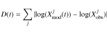
|
(2) |
with
5.1 Constraints on the model parameters using all observed species
![\begin{figure}
\par\includegraphics[width=8.5cm,clip]{13856fg12.eps}\vspace*{-2mm}
\end{figure}](/articles/aa/full_html/2010/09/aa13856-09/img51.png)
|
Figure 11: Minimum D in TMC-1 as a function of the elemental ratio C/O. The upper panel shows the results when we vary only the elemental abundances of the model, the middle panel shows the result when we vary all the parameters together, and the lower panel shows the mean and minimum values from the middle panel. |
| Open with DEXTER | |
Here we sum over all observed species to obtain D for a
given source. An important result of our analysis is that the
constraints on one specific parameter depend on the values of the other
parameters. This result is illustrated by Fig. 11, which shows three separate plots. On the left one, the minimum value of D(t)
for TMC-1 is displayed as a function of the elemental abundance
ratio C/O for the case where we vary only the elemental
abundances. The middle plot represents the same quantity but in the
case where we vary all parameters together. As can be seen on this
figure, there is a large spread for the minimum D in the middle panel, and to observe the trend better, we show on the right plot, the mean values of minimum D
obtained in this case, as well as the minimum values as a function
of elemental C/O. Although we see the same trend in both cases
that the observations in TMC-1 are better reproduced by larger values
of C/O, we also see that the best agreement (
![]() )
also exists for smaller values of elemental C/O in the case where
the other parameters are varied. In other words, the ``best
model'' is not necessarily the one at the extreme value of a parameter.
On the plots of the right of Fig. 11
for instance, the best agreement is rather flat from
C/O = 0.4 to 1.4. We can see this effect in other
instances. For example, if we only consider the agreement
with the observations as a function of the initial ratio C+/CO
while keeping the elemental abundances fixed and all the other elements
in the atomic form, we find that observations in TMC-1 are best
reproduced if all the carbon lies in the atomic form. If we change
other initial abundances, such as the initial H/H2 and/or the initial N/N2 abundance ratios, we find the best agreement for other values of the initial C+/CO.
)
also exists for smaller values of elemental C/O in the case where
the other parameters are varied. In other words, the ``best
model'' is not necessarily the one at the extreme value of a parameter.
On the plots of the right of Fig. 11
for instance, the best agreement is rather flat from
C/O = 0.4 to 1.4. We can see this effect in other
instances. For example, if we only consider the agreement
with the observations as a function of the initial ratio C+/CO
while keeping the elemental abundances fixed and all the other elements
in the atomic form, we find that observations in TMC-1 are best
reproduced if all the carbon lies in the atomic form. If we change
other initial abundances, such as the initial H/H2 and/or the initial N/N2 abundance ratios, we find the best agreement for other values of the initial C+/CO.
We will not give here the set of parameters for the ``best model'' because we did not explore the full parameter space. Doing so would be too time-consuming. The best approach for the moment is to reduce the range of possible variation of the parameters, especially for the reaction rate coefficients, which seem to be dominant for many molecules.
5.2 Constraints on the model parameters using selected species
In the previous section, we discussed some limitations on the use of
the abundances of all species observed in a cloud to constrain some of
the model parameters via the method of minimization of D.
One may do better by only using species sensitive to a given parameter
so that their sensitivity is not masked by less sensitive species.
Molecular ions, such as H3+, have been used to constrain the cosmic-ray ionization rate in diffuse regions (see for instance McCall et al. 2003; Le Petit et al. 2004). In dense clouds, the abundance ratios HCO+/CO and DCO+/HCO+ have been proposed to constrain the cosmic ray ionization rate and the fractional ionization (see for instance Caselli et al. 1998). We show in Fig. 12 the abundance ratio HCO+/CO as a function of the cosmic-ray ionization ![]() in the case where all parameters are varied at the same time. This ratio depends on time and Fig. 12 is for 105 yr,
the so-called early time of best overall agreement by number of
species. There is a clear correlation of the abundance ratio with
in the case where all parameters are varied at the same time. This ratio depends on time and Fig. 12 is for 105 yr,
the so-called early time of best overall agreement by number of
species. There is a clear correlation of the abundance ratio with ![]() but the spread of possible HCO+/CO values at a specific
but the spread of possible HCO+/CO values at a specific ![]() is at least one order of magnitude. According to Dickens et al. (2000) and Ohishi et al. (1992), the observed value of HCO+/CO is about 1.5
is at least one order of magnitude. According to Dickens et al. (2000) and Ohishi et al. (1992), the observed value of HCO+/CO is about 1.5 ![]() 10-4 in L134N and 10-4 in TMC-1 (CP). Compared with Fig. 12, these results mean that
10-4 in L134N and 10-4 in TMC-1 (CP). Compared with Fig. 12, these results mean that ![]() should be >5
should be >5 ![]() 10-17 s-1
in both clouds. The authors do not however give the uncertainties in
the observed abundances. Uncertainties should indeed be given to
improve the utility of sensitivity studies. The analysis of Caselli et al. (1998) also indicates a rather high value of
10-17 s-1
in both clouds. The authors do not however give the uncertainties in
the observed abundances. Uncertainties should indeed be given to
improve the utility of sensitivity studies. The analysis of Caselli et al. (1998) also indicates a rather high value of ![]() in TMC-1(CP) in the range (4-8)
in TMC-1(CP) in the range (4-8) ![]() 10-17 s-1. If we plot the HCO+/CO abundance ratio vs.
10-17 s-1. If we plot the HCO+/CO abundance ratio vs. ![]() ,
a parameter discussed earlier, we obtain that
,
a parameter discussed earlier, we obtain that
![]() should exceed 5
should exceed 5 ![]() 10-21 s-1 cm3.
10-21 s-1 cm3.
![\begin{figure}
\par\includegraphics[width=8.8cm,clip]{13856fg13.eps}\vspace*{-2mm}
\end{figure}](/articles/aa/full_html/2010/09/aa13856-09/img54.png)
|
Figure 12:
HCO+/CO abundance ratio as a function of |
| Open with DEXTER | |
6 Discussion
We have studied the sensitivity of the chemistry of cold dense cores to
an assortment of parameters using the 0D gas-phase model Nahoon (Wakelam et al. 2005)
in which chemical abundances evolve from given initial abundances.
As variable parameters, we considered the temperature and density
of the gas, the cosmic-ray ionization rate, the elemental
abundances, the reaction rate coefficients, and initial
concentrations. These parameters or groups of parameters were all
varied within realistic ranges of values either individually or
simultaneously using Monte Carlo methods (Vasyunin et al. 2004; Wakelam et al. 2005,2006; Vasyunin et al. 2008)
used previously mainly to study the sensitivity of molecular abundances
to chemical reaction rates. For the case of the elemental
abundances, our variations were carried out randomly from a base of
abundances based on a new set first defined in Wakelam & Herbst (2008)
as appropriate for cold dense clouds. Our results depend to some extent
upon whether individual parameters are varied while others are held
fixed at standard values or whether all parameters are varied
simultaneously.
Nevertheless, certain trends can be found. Among the most important is
the finding that, when averaged over all molecules, the dominant
source of uncertainty in predicted molecular abundances for times less
than 4 ![]() 105 yr
is the uncertainty in rate coefficients, whereas the dominant
uncertainty at later times is caused by uncertainties in elemental
abundances. The former source of uncertainty can be reduced by improved
laboratory and theoretical determinations of rate coefficients at
appropriate temperatures, especially when sensitivity analyses point
out the specific reactions of greatest importance, as done in Wakelam et al. (2009).
The latter source of uncertainty is astrophysical in origin, and
suggests that more attention be paid to a physical understanding of how
gas-phase elemental abundances evolve as dense clouds are formed from
more diffuse gas.
105 yr
is the uncertainty in rate coefficients, whereas the dominant
uncertainty at later times is caused by uncertainties in elemental
abundances. The former source of uncertainty can be reduced by improved
laboratory and theoretical determinations of rate coefficients at
appropriate temperatures, especially when sensitivity analyses point
out the specific reactions of greatest importance, as done in Wakelam et al. (2009).
The latter source of uncertainty is astrophysical in origin, and
suggests that more attention be paid to a physical understanding of how
gas-phase elemental abundances evolve as dense clouds are formed from
more diffuse gas.
Within the ranges shown in Table 3,
the sensitivity to the other parameters is generally less. As long
as the temperature and density of the gas uncertainties lie within
their listed ranges, the molecular abundances predicted by the
gas-phase model are quite robust; i.e., they do not depend much
on T and ![]() .
The only exceptions are the N-bearing species containing only nitrogen and hydrogen, such as NH3,
which are produced much less efficiently at temperatures lower than the
standard value of 10 K. Many molecular abundances depend on
the value of the cosmic-ray ionization rate, either at all times or
only between cloud ages of 104 and 107 yr. An example of the former is OH and one of the latter is HC3N, as shown in Fig. 6.
Of all the parameters, the initial concentrations with the
chosen elemental abundances seem to be the parameter to which model
results at all reasonable times are least sensitive. Nevertheless,
we found that cloud chemistry has to start with a significant
fraction of the carbon in the atomic form and a very small amount of
the hydrogen in atomic form to synthesize complex molecules.
Our standard model meets these requirements, but it may be in
conflict with with some recent 21 cm studies by Krco et al. (2009),
which show a larger amount of atomic hydrogen. The range of atomic
hydrogen abundances used when the concentrations are varied differs
strongly from the standard model in which all hydrogen starts in its
molecular form. It is thus critical to understand both the physics
and chemistry of the stages of collapse leading to the formation of
cold cores for this problem as well as the elemental abundance problem.
A new treatment of the gas-grain chemistry of cold cores in the
process of formation is being prepared by Hassel et al.
.
The only exceptions are the N-bearing species containing only nitrogen and hydrogen, such as NH3,
which are produced much less efficiently at temperatures lower than the
standard value of 10 K. Many molecular abundances depend on
the value of the cosmic-ray ionization rate, either at all times or
only between cloud ages of 104 and 107 yr. An example of the former is OH and one of the latter is HC3N, as shown in Fig. 6.
Of all the parameters, the initial concentrations with the
chosen elemental abundances seem to be the parameter to which model
results at all reasonable times are least sensitive. Nevertheless,
we found that cloud chemistry has to start with a significant
fraction of the carbon in the atomic form and a very small amount of
the hydrogen in atomic form to synthesize complex molecules.
Our standard model meets these requirements, but it may be in
conflict with with some recent 21 cm studies by Krco et al. (2009),
which show a larger amount of atomic hydrogen. The range of atomic
hydrogen abundances used when the concentrations are varied differs
strongly from the standard model in which all hydrogen starts in its
molecular form. It is thus critical to understand both the physics
and chemistry of the stages of collapse leading to the formation of
cold cores for this problem as well as the elemental abundance problem.
A new treatment of the gas-grain chemistry of cold cores in the
process of formation is being prepared by Hassel et al.
In addition to the study of model sensitivity to assorted parameters, we have utilized the simultaneous variations of these parameters to attempt to determine their optimum values by comparison of calculated and observational results for the cold cloud cores TMC-1 and L134N. In this paper, we used anindicator of agreement that minimizes the sum of the absolute values of the difference of the logarithms of the calculated and observed abundances. Constraints on individual model parameters are highly sensitive to the values of the other parameters (especially reaction rate coefficients) when variations are run simultaneously. It is currently not possible to constrain all the parameters by comparison with observed abundances by rigorous methods so that efforts have to be made to reduce the uncertainties for some of the parameters. Uncertainties in rate coefficients for instance can be reduced by laboratory measurements or theoretical calculations on reactions clearly identified as quantitatively important for the model predictions.
Finally, although the strength of sensitivity methods for gas-phase chemical models has been clearly demonstrated in this and earlier studies for both cold clouds and more complex objects such as protoplanetary disks (Vasyunin et al. 2008), the methods will need to be generalized to estimate the sensitivity to both chemical processes on grain surfaces and adsorption and desorption processes. The use of sensitivity methods for surface chemistry may become quite feasible within the next decade given the rapid pace of advance of both theory and experiments in this complex field.
AcknowledgementsWe thank the referee for his careful reading of the paper and his suggestions. E.H. acknowledges the support of the National Science Foundation (US) for the support of his program in astrochemistry, the support of the NSF Center for the Chemistry of the Universe, and the support of NASA (NAI) for his work in the evolution of pre-planetary matter. V.W. and S.G. thank the French program PCMI for partial support of this work.
References
- Bergin, E. A., Hartmann, L. W., Raymond, J. C., & Ballesteros-Paredes, J. 2004, ApJ, 612, 921 [NASA ADS] [CrossRef] [Google Scholar]
- Cardelli, J. A., Mathis, J. S., Ebbets, D. C., & Savage, B. D. 1993, ApJ, 402, L17 [NASA ADS] [CrossRef] [Google Scholar]
- Caselli, P., Walmsley, C. M., Terzieva, R., & Herbst, E. 1998, ApJ, 499, 234 [Google Scholar]
- Dickens, J. E., Irvine, W. M., Snell, R. L., et al. 2000, ApJ, 542, 870 [NASA ADS] [CrossRef] [Google Scholar]
- Flower, D. R., & Pineau des Forêts, G. 2003, MNRAS, 343, 390 [NASA ADS] [CrossRef] [Google Scholar]
- Graedel, T. E., Langer, W. D., & Frerking, M. A. 1982, ApJS, 48, 321 [NASA ADS] [CrossRef] [Google Scholar]
- Hassel, G. E., Herbst, E., & Bergin, E. A. 2010, A&A, 515, A66 [NASA ADS] [CrossRef] [EDP Sciences] [Google Scholar]
- Indriolo, N., Fields, B. D., & McCall, B. J. 2009, ApJ, 694, 257 [NASA ADS] [CrossRef] [Google Scholar]
- Jenkins, E. B. 2004, in Origin and Evolution of the Elements, 336 [Google Scholar]
- Krco, M., Goldsmith, P. F., & Brown, R. L. 2009, in BAAS, 41, 457 [Google Scholar]
- Le Bourlot, J. 1991, A&A, 242, 235 [NASA ADS] [Google Scholar]
- Le Petit, F., Roueff, E., & Herbst, E. 2004, A&A, 417, 993 [NASA ADS] [CrossRef] [EDP Sciences] [Google Scholar]
- Lee, H.-H., Herbst, E., Pineau des Forets, G., Roueff, E., & Le Bourlot, J. 1996, A&A, 311, 690 [NASA ADS] [Google Scholar]
- Lee, H.-H., Roueff, E., Pineau des Forêts, G., et al. 1998, A&A, 334, 1047 [NASA ADS] [Google Scholar]
- Lepp, S., & Dalgarno, A. 1996, A&A, 306, L21 [NASA ADS] [Google Scholar]
- McCall, B. J., Huneycutt, A. J., Saykally, R. J., et al. 2003, Nature, 422, 500 [NASA ADS] [CrossRef] [PubMed] [Google Scholar]
- Meyer, D. M., Jura, M., & Cardelli, J. A. 1998, ApJ, 493, 222 [NASA ADS] [CrossRef] [Google Scholar]
- Ohishi, M., Irvine, W. M., & Kaifu, N. 1992, in Astrochemistry of Cosmic Phenomena, IAU Symp., 150, 171 [Google Scholar]
- Osterbrock, D. E., Tran, H. D., & Veilleux, S. 1992, ApJ, 389, 305 [NASA ADS] [CrossRef] [Google Scholar]
- Padovani, M., Galli, D., & Glassgold, A. E. 2009, A&A, 501, 619 [NASA ADS] [CrossRef] [EDP Sciences] [Google Scholar]
- Ruffle, D. P., Hartquist, T. W., Caselli, P., & Williams, D. A. 1999, MNRAS, 306, 691 [NASA ADS] [CrossRef] [Google Scholar]
- Savage, B. D., & Sembach, K. R. 1996, ARA&A, 34, 279 [NASA ADS] [CrossRef] [Google Scholar]
- Shalabiea, O. M., & Greenberg, J. M. 1995, A&A, 296, 779 [NASA ADS] [Google Scholar]
- Spitzer, L. J., & Tomasko, M. G. 1968, ApJ, 152, 971 [NASA ADS] [CrossRef] [Google Scholar]
- Vasyunin, A. I., Sobolev, A. M., Wiebe, D. S., & Semenov, D. A. 2004, Astron. Lett., 30, 566 [NASA ADS] [CrossRef] [Google Scholar]
- Vasyunin, A. I., Semenov, D., Henning, T., et al. 2008, ApJ, 672, 629 [NASA ADS] [CrossRef] [Google Scholar]
- Wakelam, V., & Herbst, E. 2008, ApJ, 680, 371 [NASA ADS] [CrossRef] [Google Scholar]
- Wakelam, V., Selsis, F., Herbst, E., & Caselli, P. 2005, A&A, 444, 883 [NASA ADS] [CrossRef] [EDP Sciences] [Google Scholar]
- Wakelam, V., Herbst, E., & Selsis, F. 2006, A&A, 451, 551 [NASA ADS] [CrossRef] [EDP Sciences] [Google Scholar]
- Wakelam, V., Loison, J.-C., Herbst, E., et al. 2009, A&A, 495, 513 [NASA ADS] [CrossRef] [EDP Sciences] [Google Scholar]
- Walsh, C., Harada, N., Herbst, E., & Millar, T. J. 2009, ApJ, 700, 752 [NASA ADS] [CrossRef] [Google Scholar]
- Webber, W. R. 1998, ApJ, 506, 329 [Google Scholar]
- Wootten, A., Loren, R. B., & Snell, R. L. 1982, ApJ, 255, 160 [NASA ADS] [CrossRef] [Google Scholar]
Footnotes
- ... models
- The osu.03.2008 network is only available in electronic form at the CDS via anonymous ftp to cdsarc.u-strasbg.fr (130.79.128.5) or via http://cdsweb.u-strasbg.fr/cgi-bin/qcat?J/A+A/517/A21
All Tables
Table 1: Standard dense cloud model.
Table 2: Elemental abundances with respect to total hydrogen nuclei.
Table 3: Variational ranges of the parameters.
All Figures
|
|
Figure 1:
CO abundance computed in a diffuse/translucent cloud. Upper panel: plot of 10% of the runs. Middle panel:
the gray levels represents the percentage of runs. Any level
of gray: at least one run. Two darkest gray levels: 95% of
all runs at one given time (2 sigma if the distribution is
log-normal). Darkest gray: 68% of all runs (1 sigma if the
distribution is log-normal). Lower panel: distribution of the fractional abundance at 107 yr, where the median value is approximately 2 |
| Open with DEXTER | |
| In the text | |
| |
Figure 2: Steps used to vary all the parameters of the model collectively. |
| Open with DEXTER | |
| In the text | |
|
|
Figure 3: O2, CH, C3O and HC7N abundances as a function of time in the dense cloud stage, starting with a distribution of atomic and molecular abundances discussed in the text. The black lines represent abundances obtained if we use our standard atomic initial concentrations except for H2. |
| Open with DEXTER | |
| In the text | |
| |
Figure 4: Left panel: calculated HC3N, C5H and CH3OH abundances as a function of the initial concentration ratio C+/CO of the dense cloud stage. Right panel: calculated CH2 and HC3N abundances as a function of initial atomic hydrogen fractional abundance. Results are shown for 105 yr. |
| Open with DEXTER | |
| In the text | |
| |
Figure 5:
OH sensitivity to the cosmic-ray ionization rate ( |
| Open with DEXTER | |
| In the text | |
| |
Figure 6:
HC3N sensitivity to the cosmic-ray ionization rate ( |
| Open with DEXTER | |
| In the text | |
|
|
Figure 7: HC3N sensitivity to elemental abundances. Left panel: HC3N probability density as a function of time. Right upper panel: distribution of HC3N abundance at 107 yr. Right lower panel: HC3N abundance as a function of elemental C/O ratio at 107 yr. |
| Open with DEXTER | |
| In the text | |
|
|
Figure 8:
Logarithmic standard deviations for different parameters
|
| Open with DEXTER | |
| In the text | |
|
|
Figure 9:
Abundance of HC3N as a function of time for the case of all parameters varied together on the left and for the variation of rate coefficient only on the right. In each panel, the middle curve represents the median abundance while the two external curves represent a 1 |
| Open with DEXTER | |
| In the text | |
|
|
Figure 10: Average logarithmic standard deviation over all species for each parameter or group of parameters. The ordinate is the sum of the standard deviations of the individual molecular species divided by the number of molecular species. |
| Open with DEXTER | |
| In the text | |
|
|
Figure 11: Minimum D in TMC-1 as a function of the elemental ratio C/O. The upper panel shows the results when we vary only the elemental abundances of the model, the middle panel shows the result when we vary all the parameters together, and the lower panel shows the mean and minimum values from the middle panel. |
| Open with DEXTER | |
| In the text | |
|
|
Figure 12:
HCO+/CO abundance ratio as a function of |
| Open with DEXTER | |
| In the text | |
Copyright ESO 2010
Current usage metrics show cumulative count of Article Views (full-text article views including HTML views, PDF and ePub downloads, according to the available data) and Abstracts Views on Vision4Press platform.
Data correspond to usage on the plateform after 2015. The current usage metrics is available 48-96 hours after online publication and is updated daily on week days.
Initial download of the metrics may take a while.