| Issue |
A&A
Volume 517, July 2010
|
|
|---|---|---|
| Article Number | A26 | |
| Number of page(s) | 13 | |
| Section | Astronomical instrumentation | |
| DOI | https://doi.org/10.1051/0004-6361/200913822 | |
| Published online | 28 July 2010 | |
Poisson denoising on the sphere: application to the Fermi gamma ray space telescope
J. Schmitt1 - J. L. Starck1 - J. M. Casandjian1 - J. Fadili2 - I. Grenier1
1 - CEA, Laboratoire AIM, CEA/DSM-CNRS-Université Paris Diderot,
CEA, IRFU, Service d'Astrophysique, Centre de Saclay, 91191 Gif-Sur-Yvette Cedex, France
2 - GREYC CNRS-ENSICAEN-Université de Caen, 6 Bd du Maréchal Juin, 14050 Caen Cedex, France
Received 7 December 2009 / Accepted 8 March 2010
Abstract
The Large Area Telescope (LAT), the main instrument of the Fermi
gamma-ray Space telescope, detects high energy gamma rays with
energies from 20 MeV to more than 300 GeV. The two main
scientific objectives, the study of the Milky Way diffuse
background and the detection of point sources, are complicated by
the lack of photons. That is why we need a powerful Poisson noise
removal method on the sphere which is efficient on low count Poisson
data. This paper presents a new multiscale decomposition on the sphere
for data with Poisson noise, called multi-scale variance stabilizing
transform on the sphere (MS-VSTS). This method is based on a variance
stabilizing transform (VST), a transform which aims to
stabilize a Poisson data set such that each stabilized sample has a
quasi constant variance. In addition, for the VST used in the
method, the transformed data are asymptotically Gaussian. MS-VSTS
consists of decomposing the data into a sparse multi-scale dictionary
like wavelets or curvelets, and then applying a VST on the
coefficients in order to get almost Gaussian stabilized coefficients.
In this work, we use the isotropic undecimated wavelet transform
(IUWT) and the curvelet transform as spherical multi-scale transforms.
Then, binary hypothesis testing is carried out to detect significant
coefficients, and the denoised image is reconstructed with an iterative
algorithm based on hybrid steepest descent (HSD). To detect
point sources, we have to extract the Galactic diffuse background:
an extension of the method to background separation is then
proposed. In contrary, to study the Milky Way diffuse
background, we remove point sources with a binary mask. The gaps have
to be interpolated: an extension to inpainting is then proposed.
The method, applied on simulated Fermi LAT data, proves to be adaptive, fast and easy to implement.
Key words: methods: data analysis - techniques: image processing - gamma rays: general
1 Introduction
The Fermi gamma-ray space telescope, which was launched by NASA in June 2008, is a powerful space observatory which studies the high-energy gamma-ray sky (Atwood et al. 2009). Fermi's main instrument, the Large Area Telescope (LAT), detects photons in an energy range between 20 MeV to greater than 300 GeV. The LAT is much more sensitive than its predecessor, the EGRET telescope on the Compton Gamma Ray Observatory, and is expected to find several thousand gamma ray sources, which is an order of magnitude more than its predecessor EGRET (Hartman et al. 1999).
Even with its
![]() effective area, the number of photons detected by the
LAT outside the Galactic plane and away from intense sources is
expected to be low. Consequently, the spherical photon count
images obtained by Fermi
are degraded by the fluctuations on the number of detected photons. The
basic photon-imaging model assumes that the number of detected photons
at each pixel location is Poisson distributed. More specifically,
the image is considered as a realization of an inhomogeneous
Poisson process. This quantum noise makes the source detection more
difficult, consequently it is better to have an efficient denoising
method for spherical Poisson data.
effective area, the number of photons detected by the
LAT outside the Galactic plane and away from intense sources is
expected to be low. Consequently, the spherical photon count
images obtained by Fermi
are degraded by the fluctuations on the number of detected photons. The
basic photon-imaging model assumes that the number of detected photons
at each pixel location is Poisson distributed. More specifically,
the image is considered as a realization of an inhomogeneous
Poisson process. This quantum noise makes the source detection more
difficult, consequently it is better to have an efficient denoising
method for spherical Poisson data.
Several techniques have been proposed in the literature to estimate Poisson intensity in 2D. A major class of methods adopt a multiscale bayesian framework specifically tailored for Poisson data (Nowak & Kolaczyk 2000), independently initiated by Timmerman & Nowak (1999) and Kolaczyk (1999). Lefkimmiaits et al. (2009) proposed an improved bayesian framework for analyzing Poisson processes, based on a multiscale representation of the Poisson process in which the ratios of the underlying Poisson intensities in adjacent scales are modeled as mixtures of conjugate parametric distributions. Another approach includes preprocessing the count data by a variance stabilizing transform (VST) such as the Anscombe (1948) and the Fisz (1955) transforms, applied respectively in the spatial (Donoho 1993) or in the wavelet domain (Fryzlewicz & Nason 2004). The transform reforms the data so that the noise approximately becomes Gaussian with a constant variance. Standard techniques for independant identically distributed Gaussian noise are then used for denoising. Zhang et al. (2008) proposed a powerful method called multi-scale variance stabilizing tranform (MS-VST). It consists in combining a VST with a multiscale transform (wavelets, ridgelets or curvelets), yielding asymptotically normally distributed coefficients with known variances. The choice of the multi-scale method depends on the morphology of the data. Wavelets represent more efficiently regular structures and isotropic singularities, whereas ridgelets are designed to represent global lines in an image, and curvelets represent efficiently curvilinear contours. Significant coefficients are then detected with binary hypothesis testing, and the final estimate is reconstructed with an iterative scheme. In Starck et al. (2009), it was shown that sources can be detected in 3D LAT data (2D+time or 2D+energy) using a specific 3D extension of the MS-VST.
There is, to our knowledge, no method for Poisson intensity estimation on spherical data. It is possible to decompose the spherical data into several 2D projections, denoise each projection and reconstitute the denoised spherical data, but the projection induces some caveats like visual artifacts on the borders or deformation of the sources.
In the scope of the Fermi mission, we have two main scientific objectives:
- detection of point sources to build the catalog of gamma ray sources;
- study of the Milky Way diffuse background, which is due to interaction between cosmic rays and interstellar gas and radiation.
The aim of this paper is to introduce a Poisson denoising method on the
sphere called multi-scale variance stabilizing transform on the sphere
(MS-VSTS) in order to denoise the Fermi photon count maps. This method is based on the MS-VST (Zhang et al. 2008) and on recent on multi-scale transforms on the sphere (Abrial et al. 2007,2008; Starck et al. 2006).
Section 2 recalls the multiscale transforms on the sphere which
are used in this paper, and Gaussian denoising methods based on sparse
representations. Section 3 introduces the MS-VSTS. Section 4
applies the MS-VSTS to spherical data restoration. Section 5
applies the MS-VSTS to inpainting. Section 6 applies the MS-VSTS
to background extraction. Conclusions are drawn in Sect. 7.
In this paper, all experiments were performed on HEALPix maps with
![]() (Górski et al. 2005), which corresponds to a good pixelisation choice for the GLAST/FERMI
resolution. The performance of the method is not dependent on the nside
parameter. For a given data set, if nside is small,
it just means that we don't want to investigate the finest scales.
If nside is large, the number of counts per pixel will be
very small, and we may not have enough statistics to get any
information at the finest resolution levels. But it will not have
any bad effect on the solution. Indeed, the finest scales will be
smoothed, since our algorithm will not detect any significant wavelet
coefficients in the finest scales. Hence, starting with a fine
pixelisation (i.e. large nside), our method will provide a kind of
automatic binning, by thresholding wavelets coefficients at scales
and at spatial positions where the number of counts is not sufficient.
(Górski et al. 2005), which corresponds to a good pixelisation choice for the GLAST/FERMI
resolution. The performance of the method is not dependent on the nside
parameter. For a given data set, if nside is small,
it just means that we don't want to investigate the finest scales.
If nside is large, the number of counts per pixel will be
very small, and we may not have enough statistics to get any
information at the finest resolution levels. But it will not have
any bad effect on the solution. Indeed, the finest scales will be
smoothed, since our algorithm will not detect any significant wavelet
coefficients in the finest scales. Hence, starting with a fine
pixelisation (i.e. large nside), our method will provide a kind of
automatic binning, by thresholding wavelets coefficients at scales
and at spatial positions where the number of counts is not sufficient.
2 Multi-scale analysis on the sphere
New multi-scale transforms on the sphere were developed by Starck et al. (2006). These transforms can be inverted and are easy to compute with the HEALPix pixellisation, and were used for denoising, deconvolution, morphological component analysis and impainting applications (Abrial et al. 2007). In this paper, we use the isotropic undecimated wavelet transform (IUWT) and the curvelet transform.
2.1 Multi-scale transforms on the sphere
2.1.1 Isotropic undecimated wavelet transform on the sphere
The isotropic undecimated wavelet transform on the sphere (IUWT) is a
wavelet transform on the sphere based on the spherical harmonics
transform and with a very simple reconstruction algorithm. At
scale j, we denote
![]() the scale coefficients, and
the scale coefficients, and
![]() the wavelet coefficients, with
the wavelet coefficients, with ![]() denoting the longitude and
denoting the longitude and ![]() the latitude. Given a scale coefficient aj, the smooth coefficient aj+1 is obtained by a convolution with a low pass filter hj:
the latitude. Given a scale coefficient aj, the smooth coefficient aj+1 is obtained by a convolution with a low pass filter hj:
![]() .
The wavelet coefficients are defined by the difference between two consecutive resolutions:
dj+1 = aj - aj+1. A straightforward reconstruction is then given by:
.
The wavelet coefficients are defined by the difference between two consecutive resolutions:
dj+1 = aj - aj+1. A straightforward reconstruction is then given by:
Since this transform is redundant, the procedure for reconstructing an image from its coefficients is not unique and this can be profitably used to impose additional constraints on the synthesis functions (e.g. smoothness, positivity). A reconstruction algorithm based on a variety of filter banks is described in Starck et al. (2006).
2.1.2 Curvelet transform on the sphere
The curvelet transform enables the directional analysis of an image in
different scales. The data undergo an Isotropic Undecimated Wavelet
Transform on the sphere. Each scale j is then decomposed into smoothly overlapping blocks of side-length Bj in such a way that the overlap between two vertically adjacent blocks is a rectangular array of size Bj ![]() Bj /2, using the HEALPix pixellisation. Finally, the ridgelet transform (Candes & Donoho 1999)
is applied on each individual block. The method is best for the
detection of anisotropic structures and smooth curves and edges of
different lengths. More details can be found in Starck et al. (2006).
Bj /2, using the HEALPix pixellisation. Finally, the ridgelet transform (Candes & Donoho 1999)
is applied on each individual block. The method is best for the
detection of anisotropic structures and smooth curves and edges of
different lengths. More details can be found in Starck et al. (2006).
2.2 Application to Gaussian denoising on the sphere
Multiscale transforms on the sphere have been used successfully for
Gaussian denoising via non-linear filtering or thresholding methods.
Hard thresholding, for instance, consists of setting all insignificant
coefficients (i.e. coefficients with an absolute value below a
given threshold) to zero. In practice, we need to estimate the
noise standard deviation ![]() in each band j and a coefficient wj is significant if
in each band j and a coefficient wj is significant if
![]() ,
where
,
where ![]() is a parameter typically chosen between 3 and 5. Denoting
is a parameter typically chosen between 3 and 5. Denoting ![]() the noisy data and
the noisy data and
![]() the thresholding operator, the filtered data
the thresholding operator, the filtered data ![]() are obtained by:
are obtained by:
|
(2) |
where
3 Multi-scale variance stabilizing transform on the sphere (MS-VSTS)
3.1 Principle of VST
3.1.1 VST of a Poisson process
Given Poisson data
![]() ,
each sample
,
each sample
![]() has a variance
has a variance
![]() .
Thus, the variance of
.
Thus, the variance of ![]() is signal-dependant. The aim of a VST
is signal-dependant. The aim of a VST ![]() is to stabilize the data such that each coefficient of
is to stabilize the data such that each coefficient of
![]() has an (asymptotically) constant variance, say 1, irrespective of the value of
has an (asymptotically) constant variance, say 1, irrespective of the value of ![]() .
In addition, for the VST used in this study,
.
In addition, for the VST used in this study,
![]() is asymptotically normally distributed. Thus, the VST-transformed data are asymptotically stationary and Gaussian.
is asymptotically normally distributed. Thus, the VST-transformed data are asymptotically stationary and Gaussian.
The Anscombe (1948) transform is a widely used VST which has a simple square-root form
We can show that
It can be shown that the Anscombe VST requires a high underlying intensity to well stabilize the data (typically for
3.1.2 VST of a filtered Poisson process
Let
![]() be the filtered process obtained by convolving (Yi)i with a discrete filter h. We will use Z to denote any of the Zj's. Let us define
be the filtered process obtained by convolving (Yi)i with a discrete filter h. We will use Z to denote any of the Zj's. Let us define
![]() for
for
![]() .
In addition, we adopt a local homogeneity assumption stating that
.
In addition, we adopt a local homogeneity assumption stating that
![]() for all i within the support of h.
for all i within the support of h.
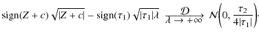
We define the square-root transform T as follows:
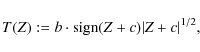
where b is a normalizing factor. Lemma 1 proves that T is a VST for a filtered Poisson process (with a nonzero-mean filter) in that T(Y) is asymptotically normally distributed with a stabilized variance as
![\begin{figure*}
\par\includegraphics[width=16cm,clip]{fig1.eps}
\end{figure*}](/articles/aa/full_html/2010/09/aa13822-09/img45.png)
|
Figure 1:
Normalized value (
|
| Open with DEXTER | |
3.2 MS-VSTS
The MS-VSTS consists in combining the square-root VST with a multi-scale transform.
3.2.1 MS-VSTS + IUWT
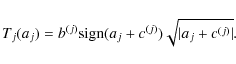
This section describes the MS-VSTS + IUWT, which is a combination of a square-root VST with the IUWT. The recursive scheme is:
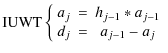
![$\displaystyle \qquad\qquad \Longrightarrow \begin{array}{l}
{\rm MS-VSTS} \\ [...
...ast a_{j-1} \\ [1mm] d_j & = & T_{j-1}(a_{j-1}) - T_j(a_j). \end{array}\right.$](/articles/aa/full_html/2010/09/aa13822-09/img47.png)
In (7), the filtering on aj-1 can be rewritten as a filtering on
Let us define
The MS-VSTS+IUWT procedure is directly invertible as we have:
![\begin{displaymath}%
a_0 (\theta,\varphi) = T_0^{-1} \Bigg[ T_J(a_J) + \sum_{j=1}^J d_j \Bigg] (\theta,\varphi).
\end{displaymath}](/articles/aa/full_html/2010/09/aa13822-09/img58.png)
Setting
where
It means that the detail coefficients issued from locally homogeneous
parts of the signal follow asymptotically a central normal distribution
with an intensity-independant variance which relies solely on the
filter h and the current scale for a given filter h. Consequently, the stabilized variances and the constants b(j), c(j),
![]() can all be pre-computed. Let us define
can all be pre-computed. Let us define
![]() the stabilized variance at scale j for a locally homogeneous part of the signal:
the stabilized variance at scale j for a locally homogeneous part of the signal:
To compute the
Table 1:
Precomputed values of the variances ![]() of the wavelet coefficients.
of the wavelet coefficients.
We have simulated Poisson images of different constant intensities ![]() ,
computed the IUWT with MS-VSTS on each image and observed the variation of the normalized value of
,
computed the IUWT with MS-VSTS on each image and observed the variation of the normalized value of
![]() (
(
![]() )
as a function of
)
as a function of ![]() for each scale j (Fig. 1). We see that the wavelet coefficients are stabilized when
for each scale j (Fig. 1). We see that the wavelet coefficients are stabilized when
![]() except for the first wavelet scale, which is mostly constituted of noise. In Fig. 2,
we compare the result of MS-VSTS with Anscombe + wavelet
shrinkage, on sources of varying intensities. We see that MS-VSTS
works well on sources of very low intensities, whereas Anscombe doesn't
work when the intensity is too low.
except for the first wavelet scale, which is mostly constituted of noise. In Fig. 2,
we compare the result of MS-VSTS with Anscombe + wavelet
shrinkage, on sources of varying intensities. We see that MS-VSTS
works well on sources of very low intensities, whereas Anscombe doesn't
work when the intensity is too low.
![\begin{figure}
\par\includegraphics[width=7.2cm,clip]{13822fg6.eps}\includegraph...
...clip]{13822fg8.eps}\includegraphics[width=7.2cm,clip]{13822fg9.eps}
\end{figure}](/articles/aa/full_html/2010/09/aa13822-09/img68.png)
|
Figure 2: Comparison of MS-VSTS with Anscombe + wavelet shrinkage on a single HEALPix face. Top left: sources of varying intensity. Top right: sources of varying intensity with Poisson noise. Bottom left: Poisson sources of varying intensity reconstructed with Anscombe + wavelet shrinkage. Bottom right: Poisson sources of varying intensity reconstructed with MS-VSTS. |
| Open with DEXTER | |
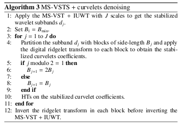
3.2.2 MS-VSTS + curvelets
As the first step of the algorithm is an IUWT, we can stabilize each resolution level as in Eq. (7). We then apply the local ridgelet transform on each stabilized wavelet band.
It is not as straightforward as with the IUWT to derive the
asymptotic noise variance in the stabilized curvelet domain.
In our experiments, we derived them using simulated Poisson data
of stationary intensity level ![]() .
After having checked that the standard deviation in the curvelet bands
becomes stabilized as the intensity level increases (which means that
the stabilization is working properly), we stored the standard
deviation
.
After having checked that the standard deviation in the curvelet bands
becomes stabilized as the intensity level increases (which means that
the stabilization is working properly), we stored the standard
deviation
![]() for each wavelet scale j and each ridgelet band l (Table 2).
for each wavelet scale j and each ridgelet band l (Table 2).
4 Poisson denoising
4.1 MS-VST + IUWT
Under the hypothesis of homogeneous Poisson intensity, the stabilized wavelet coefficients dj behave like centered Gaussian variables of standard deviation
![]() .
We can detect significant coefficients with binary hypothesis testing as in Gaussian denoising.
.
We can detect significant coefficients with binary hypothesis testing as in Gaussian denoising.
Table 2:
Asymptotic values of the variances
![]() of the curvelet coefficients.
of the curvelet coefficients.
Under the null hypothesis
![]() of homogeneous Poisson intensity, the distribution of the stabilized wavelet coefficient dj[k] at scale j and location index k can be written as:
of homogeneous Poisson intensity, the distribution of the stabilized wavelet coefficient dj[k] at scale j and location index k can be written as:
![\begin{displaymath}%
p(d_j[k]) = \frac{1}{\sqrt{2\pi}\sigma_j}\exp(-d_j[k]^2 / 2 \sigma_j^2).
\end{displaymath}](/articles/aa/full_html/2010/09/aa13822-09/img71.png)
|
(13) |
The rejection of the hypothesis
![\begin{displaymath}%
p_j[k] = 2 \frac{1}{\sqrt{2\pi}\sigma_j}\int_{\vert d_j[k]\vert}^{+\infty} \exp(-x^2 / 2 \sigma_j^2){\rm d}x.
\end{displaymath}](/articles/aa/full_html/2010/09/aa13822-09/img72.png)
|
(14) |
Consequently, to accept or reject
- if
![$\vert d_j[k]\vert \geqslant \kappa \sigma_j$](/articles/aa/full_html/2010/09/aa13822-09/img75.png) ,
dj[k] is significant;
,
dj[k] is significant;
- if
![$\vert d_j[k]\vert < \kappa \sigma_j$](/articles/aa/full_html/2010/09/aa13822-09/img76.png) ,
dj[k] is not significant.
,
dj[k] is not significant.
We define the multiresolution support
![]() ,
which is determined by the set of detected significant coefficients after hypothesis testing:
,
which is determined by the set of detected significant coefficients after hypothesis testing:
![\begin{displaymath}%
\mathcal{M} := (j,k) \vert {\rm if }~d_j[k]~{\rm is~declared~significant}.
\end{displaymath}](/articles/aa/full_html/2010/09/aa13822-09/img78.png)
We formulate the reconstruction problem as a convex constrained minimization problem:
![\begin{displaymath}%
{\rm Arg} \min_{\vec{X}} \Vert \mathbf{ \Phi}^{T}\vec{X}\Ve...
...{X})_j[k]=(\mathbf{ \Phi}^{T}\vec{Y})_j[k], \end{array}\right.
\end{displaymath}](/articles/aa/full_html/2010/09/aa13822-09/img79.png)
where
This problem is solved with the following iterative scheme: the image is initialised by
![]() ,
and the iteration scheme is, for n=0 to
,
and the iteration scheme is, for n=0 to
![]() :
:
| (17) | ||
| (18) |
where P+ denotes the projection on the positive orthant,
![\begin{displaymath}%
P_{\mathcal{M}}d_j[k] = \left\{\begin{array}{cc} d_j[k] & {...
...) \in \mathcal{M}, \\ 0 & {\rm otherwise}. \end{array} \right.
\end{displaymath}](/articles/aa/full_html/2010/09/aa13822-09/img85.png)
|
(19) |
and
![\begin{displaymath}%
{\rm ST}_{\lambda_n} [d] = \left\{\begin{array}{cc} {\rm si...
...eqslant \lambda_n, \\ 0 & {\rm otherwise}. \end{array} \right.
\end{displaymath}](/articles/aa/full_html/2010/09/aa13822-09/img88.png)
|
(20) |
We chose a decreasing threshold
The final estimate of the Poisson intensity is:
![]() .
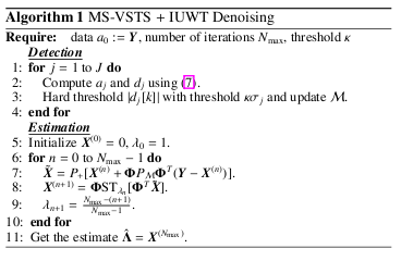
Algorithm 1 summarizes the main steps of the MS-VSTS + IUWT denoising algorithm.
.
Algorithm 1 summarizes the main steps of the MS-VSTS + IUWT denoising algorithm.
4.2 Multi-resolution support adaptation
When two sources are too close, the less intense source may not be detected because of the negative wavelet coefficients of the brightest source. To avoid such a drawback, we may update the multi-resolution support at each iteration. The idea is to withdraw the detected sources and to make a detection on the remaining residual, so as to detect the sources which may have been missed at the first detection.
At each iteration n, we compute the MS-VSTS of
![]() .
We denote
d(n)j[k] the stabilised coefficients of
.
We denote
d(n)j[k] the stabilised coefficients of
![]() .
We make a hard thresholding on
(dj[k]-d(n)j[k]) with the same thresholds as in the detection step. Significant coefficients are added to the multiresolution support
.
We make a hard thresholding on
(dj[k]-d(n)j[k]) with the same thresholds as in the detection step. Significant coefficients are added to the multiresolution support
![]() .
.
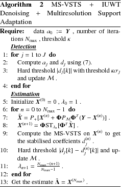
The main steps of the algorithm are summarized in Algorithm 2. In practice, we use Algorithm 2 instead of Algorithm 1 in our experiments.
4.3 MS-VST + Curvelets
Insignificant coefficients are zeroed by using the same hypothesis
testing framework as in the wavelet scale. At each wavelet
scale j and ridgelet band k, we make a hard thresholding on curvelet coefficients with threshold
![]() ,
,
![]() or 5. Finally, a direct reconstruction can be performed by
first inverting the local ridgelet transforms and then inverting the
MS-VST + IUWT (Equation (10)). An iterative reconstruction may also be performed.
or 5. Finally, a direct reconstruction can be performed by
first inverting the local ridgelet transforms and then inverting the
MS-VST + IUWT (Equation (10)). An iterative reconstruction may also be performed.
Algorithm 3 summarizes the main steps of the MS-VSTS + Curvelets denoising algorithm.
![\begin{figure}
\par\includegraphics[width=7.5cm,clip]{13822fg10.eps}\hspace*{1mm...
...eps}\hspace*{1mm}
\includegraphics[width=7.5cm,clip]{13822fg15.eps}
\end{figure}](/articles/aa/full_html/2010/09/aa13822-09/img96.png)
|
Figure 3:
Top left: Fermi simulated map without noise. Top right: Fermi simulated map with Poisson noise. Middle left: Fermi simulated map denoised with Anscombe VST + wavelet shrinkage. Middle right: Fermi simulated map denoised with MS-VSTS + curvelets (Algorithm 3). Bottom left: Fermi simulated map denoised with MS-VSTS + IUWT (Algorithm 1) with threshold |
| Open with DEXTER | |
4.4 Experiments
The method was tested on simulated Fermi data. The simulated
data are the sum of a Milky Way diffuse background model and
1000 gamma ray point sources. We based our Galactic diffuse
emission model intensity on the model
![]() obtained at the Fermi Science Support Center (Myers 2009).
This model results from a fit of the LAT photons with various gas
templates as well as inverse Compton in several energy bands. We used a
realistic point-spread function for the sources, based on
Monte Carlo simulations of the LAT and accelerator tests, that
scale approximately as
obtained at the Fermi Science Support Center (Myers 2009).
This model results from a fit of the LAT photons with various gas
templates as well as inverse Compton in several energy bands. We used a
realistic point-spread function for the sources, based on
Monte Carlo simulations of the LAT and accelerator tests, that
scale approximately as
![]() degrees. The position of the 205 brightest sources were taken from the Fermi 3-month source list (Abdo et al. 2009). The position of the 795 remaining sources follow the LAT 1-year Point Source Catalog (Myers 2010) sources distribution: each simulated source was randomly sorted in a box of
degrees. The position of the 205 brightest sources were taken from the Fermi 3-month source list (Abdo et al. 2009). The position of the 795 remaining sources follow the LAT 1-year Point Source Catalog (Myers 2010) sources distribution: each simulated source was randomly sorted in a box of ![]() = 5
= 5![]() and
and ![]() = 1
= 1![]() around a LAT 1-year catalog source. We simulated each source
assuming a power-law dependence with its spectral index given by the
3-month source list and the first year catalog. We used an exposure of
3
around a LAT 1-year catalog source. We simulated each source
assuming a power-law dependence with its spectral index given by the
3-month source list and the first year catalog. We used an exposure of
3 ![]()
![]() corresponding approximatively to one year of Fermi
all-sky survey around 1 GeV. The simulated counts map shown
here correspond to photons energy from 150 MeV
to 20 GeV.
corresponding approximatively to one year of Fermi
all-sky survey around 1 GeV. The simulated counts map shown
here correspond to photons energy from 150 MeV
to 20 GeV.
Figure 3 compares the result of denoising with MS-VST + IUWT (Algorithm 1), MS-VST + curvelets (Algorithm 3) and Anscombe VST + wavelet shrinkage on a simulated Fermi map. Figure 4
shows one HEALPix face of the results. As expected from
theory, the Anscombe method produces poor results to denoise Fermi data,
because the underlyning intensity is too weak. Both wavelet and
curvelet denoising on the sphere perform much better. For this
application, wavelets are slightly better than curvelets (
![]() ,
,
![]() ,
,
![]() ).
As this image contains many point sources, thisresult is expected.
Indeed wavelet are better than curvelets to represent isotropic
objects.
).
As this image contains many point sources, thisresult is expected.
Indeed wavelet are better than curvelets to represent isotropic
objects.
![\begin{figure}
\par\includegraphics[width=7.5cm,clip]{13822fg16.eps}\hspace*{1mm...
...eps}\hspace*{1mm}
\includegraphics[width=7.5cm,clip]{13822fg21.eps}
\end{figure}](/articles/aa/full_html/2010/09/aa13822-09/img106.png)
|
Figure 4:
View of a single HEALPix face from the results of Fig. 3. Top left: Fermi simulated map without noise. Top right: Fermi simulated map with Poisson noise. Middle left: Fermi simulated map denoised with Anscombe VST + wavelet shrinkage. Middle right: Fermi simulated map denoised with MS-VSTS + curvelets (Algorithm 3).
Bottom left: Fermi simulated map denoised with MS-VSTS + IUWT (Algorithm 1) with threshold |
| Open with DEXTER | |
5 Milky Way diffuse background study: denoising and inpainting
In order to extract from the Fermi photon maps the galactic diffuse emission, we want to remove the point sources from the Fermi image. As our HSD algorithm is very close to the MCA algorithm (Starck et al. 2004), an idea is to mask the most intense sources and to modify our algorithm in order to interpolate through the gaps exactly as in the MCA-Inpainting algorithm (Abrial et al. 2007). This modified algorithm can be called MS-VSTS-Inpainting algorithm.
The problem can be reformulated as a convex constrained minimization problem:
![$\displaystyle \qquad\qquad \: \left\{\begin{array}{c}\vec{X} \geqslant 0, \\ \...
...Phi}^{T}\Pi \vec{X})_j[k]=(\mathbf{ \Phi}^{T} \vec{Y})_j[k], \end{array}\right.$](/articles/aa/full_html/2010/09/aa13822-09/img108.png)
where
![\begin{figure}
\par\includegraphics[width=7.5cm,clip]{13822fg22.eps}\hspace*{1mm}
\includegraphics[width=7.5cm,clip]{13822fg23.eps}
\vspace*{5mm}
\end{figure}](/articles/aa/full_html/2010/09/aa13822-09/img110.png)
|
Figure 5: MS-VSTS - Inpainting. Left: Fermi simulated map with Poisson noise and the most luminous sources masked. Right: Fermi simulated map denoised and inpainted with wavelets (Algorithm 4). Pictures are in logarithmic scale. |
| Open with DEXTER | |
The iterative scheme can be adapted to cope with a binary mask, which gives:
| (22) | |||
| (23) |
The thresholding strategy has to be adapted. Indeed, for the impainting task we need to have a very large initial threshold in order to have a very smooth image in the beginning and to refine the details progressively. We chose an exponentially decreasing threshold:
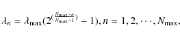
where
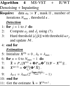
6.2 Experiment
We applied this method on simulated Fermi data where we masked the most luminous sources.
The results are in Fig. 5. The MS-VST + IUWT + Inpainting method (Algorithm 4) interpolates the missing data very well. Indeed, the missing part can not be seen anymore in the inpainted map, which shows that the diffuse emission component has been correctly reconstructed.
6 Source detection: denoising and background modeling
6.1 Method
In the case of Fermi data, the diffuse gamma-ray emission from the Milky Way, due to interaction between cosmic rays and interstellar gas and radiation, makes a relatively intense background. We have to extract this background in order to detect point sources. This diffuse interstellar emission can be modelled by a linear combination of gas templates and inverse compton map. We can use such a background model and incorporate a background removal in our denoising algorithm.
We note ![]() the data,
the data, ![]() the background we want to remove, and
d(b)j[k] the MS-VSTS coefficients of
the background we want to remove, and
d(b)j[k] the MS-VSTS coefficients of ![]() at scale j and position k. We determine the multi-resolution support by comparing
|dj[k]-d(b)j[k]| with
at scale j and position k. We determine the multi-resolution support by comparing
|dj[k]-d(b)j[k]| with
![]() .
.
We formulate the reconstruction problem as a convex constrained minimization problem:
![$\displaystyle \qquad \qquad \: \left\{\begin{array}{c}\vec{X} \geqslant 0, \\ ...
...}\vec{X})_j[k]=(\mathbf{ \Phi}^{T}(\vec{Y} - \vec{B}))_j[k]. \end{array}\right.$](/articles/aa/full_html/2010/09/aa13822-09/img117.png)
Then, the reconstruction algorithm scheme becomes:
| (26) | ||
| (27) |
The algorithm is illustrated by the theoretical study in Fig. 6. We denoise Poisson data while separating a single source, which is a Gaussian of standard deviation equal to 0.01, from a background, which is a sum of two Gaussians of standard deviation equal to 0.1 and 0.01 respectively.
![\begin{figure}
\par\includegraphics[width=7.3cm,clip]{13822fg24.eps}\hspace*{1mm...
...eps}\hspace*{1mm}
\includegraphics[width=7.3cm,clip]{13822fg27.eps}
\end{figure}](/articles/aa/full_html/2010/09/aa13822-09/img120.png)
|
Figure 6: Theoretical testing for MS-VSTS + IUWT denoising + background removal algorithm (Algorithm 5). View on a single HEALPix face. Top left: simulated background: sum of two Gaussians of standard deviation equal to 0.1 and 0.01 respectively. Top right: simulated source: Gaussian of standard deviation equal to 0.01. Bottom left: simulated poisson data. Bottom right: image denoised with MS-VSTS + IUWT and background removal. |
| Open with DEXTER | |
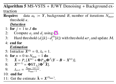
Like Algorithm 1, Algorithm 5 can be adapted to make multiresolution support adaptation.
Experiment
We applied Algorithms 5 on simulated Fermi data. To test the efficiency of our method, we detect the sources with the SExtractor routine (Bertin & Arnouts 1996), and compare the detected sources with the theoretical sources catalog to get the number of true and false detections. Results are shown in Figs. 7 and 8. The SExtractor method was applied on the first wavelet scale of the reconstructed map, with a detection threshold equal to 1. It has been chosen to optimise the number of true detections. SExtractor makes 593 true detections and 71 false detections on the Fermi simulated map restored with Algorithm 2 among the 1000 sources of the simulation. On noisy data, many fluctuations due to Poisson noise are detected as sources by SExtractor, which leads to a big number of false detections (more than 2000 in the case of Fermi data).
![\begin{figure}
\par\includegraphics[width=7.5cm,clip]{13822fg28.eps}\hspace*{1mm...
...cs[width=7.5cm,clip]{13822fg32.eps}\hspace*{3.75cm}}\vspace*{6mm}
\end{figure}](/articles/aa/full_html/2010/09/aa13822-09/img122.png)
|
Figure 7:
Top left: simulated background model. Top right: simulated gamma ray sources. Middle left: simulated Fermi data with Poisson noise. Middle right: reconstructed gamma ray sources with MS-VSTS + IUWT + background removal (Algorithm 5) with threshold |
| Open with DEXTER | |
![\begin{figure}
\par\includegraphics[width=7.5cm,clip]{13822fg33.eps}\hspace*{1mm...
...\includegraphics[width=7.5cm,clip]{13822fg37.eps}\hspace*{3.75cm}}\end{figure}](/articles/aa/full_html/2010/09/aa13822-09/img123.png)
|
Figure 8:
View of a single HEALPix face from the results of Fig. 7. Top left: simulated background model. Top right: simulated gamma ray sources. Middle left: simulated Fermi data with Poisson noise. Middle right: reconstructed gamma ray sources with MS-VSTS + IUWT + background removal (Algorithm 5) with threshold |
| Open with DEXTER | |
6.2.1 Sensitivity to model errors
As it is difficult to model the background precisely, it is
important to study the sensitivity of the method to model errors. We
add a stationary Gaussian noise to the background model, we compute the
MS-VSTS + IUWT with threshold ![]() on the simulated Fermi
Poisson data with extraction of the noisy background, and we study the
percent of true and false detections with respect to the total number
of sources of the simulation and the signal-noise ratio (
on the simulated Fermi
Poisson data with extraction of the noisy background, and we study the
percent of true and false detections with respect to the total number
of sources of the simulation and the signal-noise ratio (
![]() )
versus the standard deviation of the Gaussian perturbation. Table 3
shows that, when the standard deviation of the noise on the background
model becomes of the same range as the mean of the Poisson intensity
distribution (
)
versus the standard deviation of the Gaussian perturbation. Table 3
shows that, when the standard deviation of the noise on the background
model becomes of the same range as the mean of the Poisson intensity
distribution (
![]() ),
the number of false detections increases, the number of true
detections decreases and the signal noise ratio decreases. While the
perturbation is not too strong (standard deviation <10), the
effect of the model error remains low.
),
the number of false detections increases, the number of true
detections decreases and the signal noise ratio decreases. While the
perturbation is not too strong (standard deviation <10), the
effect of the model error remains low.
Table 3: Percent of true and false detection and signal-noise ratio versus the standard deviation of the Gaussian noise on the background model.
7 Conclusion
This paper presented new methods for restoration of spherical data with noise following a Poisson distribution. A denoising method was proposed, which used a variance stabilization method and multiscale transforms on the sphere. Experiments have shown it is very efficient for Fermi data denoising. Two spherical multiscale transforms, the wavelet and the curvelets, were used. Then, we have proposed an extension of the denoising method in order to take into account missing data, and we have shown that this inpainting method could be a useful tool to estimate the diffuse emission. Finally, we have introduced a new denoising method the sphere which takes into account a background model. The simulated data have shown that it is relatively robust to errors in the model, and can therefore be used for Fermi diffuse background modeling and source detection.
AcknowledgementsThis work was partially supported by the European Research Council grant ERC-228261.
References
- Abdo, A. A., Ackermann, M., Ajello, M., et al. 2009, ApJS, 183, 46 [NASA ADS] [CrossRef] [Google Scholar]
- Abrial, P., Moudden, Y., Starck, J., et al. 2007, Journal of Fourier Analysis and Applications, 13, 729 [Google Scholar]
- Abrial, P., Moudden, Y., Starck, J., et al. 2008, Statistical Methodology, 5, 289 [Google Scholar]
- Anscombe, F. 1948, Biometrika, 35, 246 [Google Scholar]
- Atwood, W. B., Abdo, A. A., Ackermann, M., et al. 2009, ApJ, 697, 1071 [NASA ADS] [CrossRef] [Google Scholar]
- Bertin, E., & Arnouts, S. 1996, A&AS, 117, 393 [NASA ADS] [CrossRef] [EDP Sciences] [Google Scholar]
- Candes, E., & Donoho, D. 1999, Phil. Trans. R. Soc. Lond. A, 357, 2495 [Google Scholar]
- Donoho, D. 1993, Proc. Symp. Appl. Math., 47, 173 [Google Scholar]
- Fisz, M. 1955, Colloq. Math., 3, 138 [Google Scholar]
- Fryzlewicz, P., & Nason, G. 2004, J. Comp. Graph. Stat., 13, 621 [CrossRef] [Google Scholar]
- Górski, K. M., Hivon, E., Banday, A. J., et al. 2005, ApJ, 622, 759 [NASA ADS] [CrossRef] [Google Scholar]
- Hartman, R. C., Bertsch, D. L., Bloom, S. D., et al. 1999, VizieR Online Data Catalog, 212, 30079 [NASA ADS] [Google Scholar]
- Kolaczyk, E. 1999, J. Amer. Stat. Assoc., 94, 920 [CrossRef] [Google Scholar]
- Lefkimmiaits, S., Maragos, P., & Papandreou, G. 2009, IEEE Transactions on Image Processing, 20, 20 [Google Scholar]
- Myers, J. 2009, LAT Background Models, http://fermi.gsfc.nasa.gov/ssc/data/access/lat/BackgroundModels.html [Google Scholar]
- Myers, J. 2010, LAT 1-year Point Source Catalog, http://fermi.gsfc.nasa.gov/ssc/data/access/lat/1yr_catalog/ [Google Scholar]
- Nowak, R., & Kolaczyk, E. 2000, IEEE Trans. Inf. Theory, 45, 1811 [CrossRef] [Google Scholar]
- Starck, J., Fadili, J. M., Digel, S., Zhang, B., & Chiang, J. 2009, A&A, 504, 641 [NASA ADS] [CrossRef] [EDP Sciences] [Google Scholar]
- Starck, J.-L., Elad, M., & Donoho, D. 2004, Advances in Imaging and Electron Physics, 132 [Google Scholar]
- Starck, J.-L., Moudden, Y., Abrial, P., & Nguyen, M. 2006, A&A, 446, 1191 [NASA ADS] [CrossRef] [EDP Sciences] [Google Scholar]
- Timmerman, K., & Nowak, R. 1999, IEEE Trans. Inf. Theory, 45, 846 [CrossRef] [Google Scholar]
- Yamada, I. 2001, in Inherently Parallel Algorithm in Feasibility and Optimization and their Applications (Elsevier), 473 [Google Scholar]
- Zhang, B., Fadili, J., & Starck, J.-L. 2008, IEEE Transactions on Image Processing, 11, 1093 [NASA ADS] [CrossRef] [Google Scholar]
All Tables
Table 1:
Precomputed values of the variances ![]() of the wavelet coefficients.
of the wavelet coefficients.
Table 2:
Asymptotic values of the variances
![]() of the curvelet coefficients.
of the curvelet coefficients.
Table 3: Percent of true and false detection and signal-noise ratio versus the standard deviation of the Gaussian noise on the background model.
All Figures
|
|
Figure 1:
Normalized value (
|
| Open with DEXTER | |
| In the text | |
|
|
Figure 2: Comparison of MS-VSTS with Anscombe + wavelet shrinkage on a single HEALPix face. Top left: sources of varying intensity. Top right: sources of varying intensity with Poisson noise. Bottom left: Poisson sources of varying intensity reconstructed with Anscombe + wavelet shrinkage. Bottom right: Poisson sources of varying intensity reconstructed with MS-VSTS. |
| Open with DEXTER | |
| In the text | |
|
|
Figure 3:
Top left: Fermi simulated map without noise. Top right: Fermi simulated map with Poisson noise. Middle left: Fermi simulated map denoised with Anscombe VST + wavelet shrinkage. Middle right: Fermi simulated map denoised with MS-VSTS + curvelets (Algorithm 3). Bottom left: Fermi simulated map denoised with MS-VSTS + IUWT (Algorithm 1) with threshold |
| Open with DEXTER | |
| In the text | |
|
|
Figure 4:
View of a single HEALPix face from the results of Fig. 3. Top left: Fermi simulated map without noise. Top right: Fermi simulated map with Poisson noise. Middle left: Fermi simulated map denoised with Anscombe VST + wavelet shrinkage. Middle right: Fermi simulated map denoised with MS-VSTS + curvelets (Algorithm 3).
Bottom left: Fermi simulated map denoised with MS-VSTS + IUWT (Algorithm 1) with threshold |
| Open with DEXTER | |
| In the text | |
|
|
Figure 5: MS-VSTS - Inpainting. Left: Fermi simulated map with Poisson noise and the most luminous sources masked. Right: Fermi simulated map denoised and inpainted with wavelets (Algorithm 4). Pictures are in logarithmic scale. |
| Open with DEXTER | |
| In the text | |
|
|
Figure 6: Theoretical testing for MS-VSTS + IUWT denoising + background removal algorithm (Algorithm 5). View on a single HEALPix face. Top left: simulated background: sum of two Gaussians of standard deviation equal to 0.1 and 0.01 respectively. Top right: simulated source: Gaussian of standard deviation equal to 0.01. Bottom left: simulated poisson data. Bottom right: image denoised with MS-VSTS + IUWT and background removal. |
| Open with DEXTER | |
| In the text | |
|
|
Figure 7:
Top left: simulated background model. Top right: simulated gamma ray sources. Middle left: simulated Fermi data with Poisson noise. Middle right: reconstructed gamma ray sources with MS-VSTS + IUWT + background removal (Algorithm 5) with threshold |
| Open with DEXTER | |
| In the text | |
|
|
Figure 8:
View of a single HEALPix face from the results of Fig. 7. Top left: simulated background model. Top right: simulated gamma ray sources. Middle left: simulated Fermi data with Poisson noise. Middle right: reconstructed gamma ray sources with MS-VSTS + IUWT + background removal (Algorithm 5) with threshold |
| Open with DEXTER | |
| In the text | |
Copyright ESO 2010
Current usage metrics show cumulative count of Article Views (full-text article views including HTML views, PDF and ePub downloads, according to the available data) and Abstracts Views on Vision4Press platform.
Data correspond to usage on the plateform after 2015. The current usage metrics is available 48-96 hours after online publication and is updated daily on week days.
Initial download of the metrics may take a while.