| Issue |
A&A
Volume 517, July 2010
|
|
|---|---|---|
| Article Number | A10 | |
| Number of page(s) | 7 | |
| Section | Extragalactic astronomy | |
| DOI | https://doi.org/10.1051/0004-6361/200913622 | |
| Published online | 23 July 2010 | |
The radio-X-ray luminosity correlation of radio halos at low radio frequency
Application of the turbulent re-acceleration model
R. Cassano
INAF - Istituto di Radioastronomia, via P. Gobetti 101, 40129 Bologna, Italy
Received 8 November 2009 / Accepted 6 April 2010
Abstract
Aims. We show expectations on the radio-X-ray luminosity
correlation of radio halos at 120 MHz. According to the turbulent
re-acceleration scenario, we expect that low-frequency observations can
detect a new population of radio halos that due to their ultra-steep
spectra are missed by present observations at ![]() GHz
frequencies. These radio halos are also supposed to be less luminous
than presently observed halos hosted in clusters with the same X-ray
luminosity.
GHz
frequencies. These radio halos are also supposed to be less luminous
than presently observed halos hosted in clusters with the same X-ray
luminosity.
Methods. With Monte Carlo procedures we show that these
ultra-steep spectrum halos at 120 MHz cause a steepening and a
broadening of the correlation between the synchrotron power and the
cluster X-ray luminosity with respect to that observed at 1.4 GHz.
Results. We investigate the role of future low-frequency radio
surveys and find that the upcoming LOFAR surveys will be able to test
these expectations.
Key words: radiation mechanisms: non-thermal - galaxies: clusters: general - radio continuum: general - X-rays: general
1 Introduction
Radio halos are diffuse synchrotron sources of the intra-cluster medium (ICM) extended on a mega-parsec scale (e.g., Feretti 2005; Ferrari et al. 2008). They provide the most important evidence of non-thermal components (relativistic particles and magnetic fields) mixed with the hot ICM. Galaxy clusters hosting radio halos are always characterized by a non-relaxed dynamical status suggestive of recent or ongoing merger events (e.g., Buote 2001; Schuecker et al 2001; Govoni et al. 2004; Venturi et al. 2008; Giacintucci et al. 2009). Furhermore, the halo-radio power at 1.4 GHz increases with the cluster's X-ray luminosity, mass, and temperature (e.g., Liang et al. 2000; Enßlin & Röttgering 2002; Bacchi et al. 2003; Clarke 2005; Dolag et al. 2005; Cassano et al. 2006, 2007; Brunetti et al. 2009; Rudnick & Lemmerman 2009; Giovannini et al. 2009). These correlations and the radio halo-merger connection suggest that gravity provides the reservoir of energy to generate the non-thermal components (e.g., Kempner & Sarazin 2001). Cluster mergers drive shocks and turbulence in the ICM that may amplify the magnetic fields (e.g., Carilli & Taylor 2002; Dolag et al. 2002; Brüggen et al. 2005; Subramanian et al. 2006; Ryu et al. 2008) and accelerate high-energy particles (e.g., Fujita et al. 2003; Hoeft & Brüggen 2007; Brunetti & Lazarian 2007; Pfrommer et al. 2008; Vazza et al. 2009).
Two main scenarios have been proposed to explain the origin of relativistic particles in radio halos, namely i) the turbulent re-acceleration model, in which relativistic electrons are re-energized in situ due to the interaction with MHD turbulence generated in the ICM during cluster mergers (e.g., Brunetti et al. 2001; Petrosian et al. 2001), and ii) the secondary electron models, in which the relativistic electrons are secondary products of the collisions between cosmic rays and thermal protons in the ICM (e.g., Dennison 1980; Blasi & Colafrancesco 1999; Pfrommer & Enßlin 2004).
Observations provide support to the idea that turbulence may play a role in the particle re-acceleration process (e.g., Brunetti et al. 2008; Ferrari et al. 2008; Cassano 2009; Giovannini et al. 2009), in which case the population of radio halos is predicted to be a mixture of sources with different spectral properties, with halos with steeper spectra in the majority (Cassano et al. 2006, hereafter C06; Cassano et al. 2009, hereafter C09). That is why upcoming observations with the Low Frequency Array (LOFAR) and the Long Wavelength Array (LWA) will be crucial because very steep spectrum halos should glow up at low radio frequency.
We discuss how such a predicted population is expected to
affect the properties of the radio-X-ray luminosity correlation at low
radio frequency and investigate the potential of LOFAR surveys.
A ![]() CDM cosmology (
CDM cosmology (
![]() ,
,
![]() ,
,
![]() )
is adopted.
)
is adopted.
2 The population of ultra-steep spectrum radio halos
The formation and evolution of radio halos according to the turbulent re-acceleration scenario have been investigated by means of Monte Carlo based procedures (Cassano & Brunetti 2005;
C06; C09). These procedures allow us to account for the main components
of the model, i.e., the rate of cluster-cluster mergers in the
Universe, their mass ratio, and the fraction of energy dissipated
during mergers that is channelled into MHD turbulence and acceleration
of relativistic particles.
We simulate the formation history of ![]() 1000 galaxy clusters with present day-masses in the range
1000 galaxy clusters with present day-masses in the range
![]()
![]() .
.
Turbulence acceleration is a rather inefficient process in the ICM and
electrons can be accelerated up to energy of several GeV, because at
higher energy the radiation losses dominate (e.g., Brunetti &
Lazarian 2007).
This implies a gradual spectral steepening at high frequencies in the
synchrotron spectrum of radio halos. This steepening makes it difficult
to detect radio halos at frequencies higher than the frequency
![]() at which the steepening becomes severe.
at which the steepening becomes severe.
Following C06 and C09 we use homogeneous models that assume i) an average value of the magnetic field strength in the radio-halo volume that scales with the cluster mass as
![]()
![]()
![]() , ii) that a fraction,
, ii) that a fraction,
![]() ,
of the
,
of the
![]() work, done by subclusters crossing the main clusters during mergers, goes into magneto-acoustic turbulence. The frequency
work, done by subclusters crossing the main clusters during mergers, goes into magneto-acoustic turbulence. The frequency
![]() ,
defined as the frequency at which the spectral slope of the halos becomes
,
defined as the frequency at which the spectral slope of the halos becomes
![]() (
(
![]() ), depends on the acceleration efficiency in the ICM,
), depends on the acceleration efficiency in the ICM, ![]() ,
on the magnetic field in the ICM, B, and on the energy density of the cosmic microwave background radiation (CMB) as:
,
on the magnetic field in the ICM, B, and on the energy density of the cosmic microwave background radiation (CMB) as:
![]() .
The frequency
.
The frequency
![]() is a more practical re-definition of the synchrotron-break frequency,
is a more practical re-definition of the synchrotron-break frequency,
![]() ,
and is
,
and is
![]() in homogeneous models (C09). According to C09, for a single major merger between a cluster of mass
in homogeneous models (C09). According to C09, for a single major merger between a cluster of mass ![]() and a subcluster with mass
and a subcluster with mass ![]() ,
,
![]() is
is
where
![]() is the equivalent magnetic field strength of the CMB, and
is the equivalent magnetic field strength of the CMB, and ![]() is the cluster virial radius. It is expected that mergers may generate halos with higher
is the cluster virial radius. It is expected that mergers may generate halos with higher
![]() in more massive clusters, and that halos in clusters with the same mass
in more massive clusters, and that halos in clusters with the same mass ![]() (and magnetic field) and redshift could have different
(and magnetic field) and redshift could have different
![]() depending on the properties of the merger event responsible for their generation.
Halos with
depending on the properties of the merger event responsible for their generation.
Halos with
![]() 1.4 GHz must be generated in connection with the most energetic
merger-events in the Universe because only these mergers may allow for
the efficient acceleration that is necessary to have relativistic
electrons emitting at these frequencies. Present surveys carried out at
1.4 GHz must be generated in connection with the most energetic
merger-events in the Universe because only these mergers may allow for
the efficient acceleration that is necessary to have relativistic
electrons emitting at these frequencies. Present surveys carried out at
![]() 1 GHz detect radio halos only in the most massive and merging clusters (e.g., Buote 2001; Venturi et al. 2008). On the other hand, radio halos with lower values of
1 GHz detect radio halos only in the most massive and merging clusters (e.g., Buote 2001; Venturi et al. 2008). On the other hand, radio halos with lower values of
![]() must be more common, because they can be generated in connection with
less energetic phenomena, e.g., major mergers between less massive
systems or minor mergers in massive systems, which are more frequent in
the Universe. This has been addressed quantitatively by means of Monte
Carlo calculations, which allow us to derive the fraction of clusters
with radio halos with different
must be more common, because they can be generated in connection with
less energetic phenomena, e.g., major mergers between less massive
systems or minor mergers in massive systems, which are more frequent in
the Universe. This has been addressed quantitatively by means of Monte
Carlo calculations, which allow us to derive the fraction of clusters
with radio halos with different
![]() as a function of the cluster mass and redshift. The expected population
of radio halos is indeed constituted by a mixture of halos with
different spectra, with steep spectrum halos being more common in the
Universe;
as a function of the cluster mass and redshift. The expected population
of radio halos is indeed constituted by a mixture of halos with
different spectra, with steep spectrum halos being more common in the
Universe; ![]() 200 radio halos with
200 radio halos with
![]() MHz are expected in future LOFAR surveys at 120 MHz (C09).
MHz are expected in future LOFAR surveys at 120 MHz (C09).
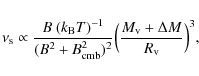
According to this model the monochromatic luminosity of radio halos at a given frequency
![]() increases with increasing
increases with increasing
![]() .
For a fixed cluster mass (or X-ray luminosity), the relation between the radio luminosity at
.
For a fixed cluster mass (or X-ray luminosity), the relation between the radio luminosity at ![]() of halos with
of halos with
![]() and
and
![]() ,
,
![]() and
and
![]() respectively, is (C09)
respectively, is (C09)

where
![]() (e.g., Ferrari et al. 2008) is the radio spectral index. A correlation between the radio power
(e.g., Ferrari et al. 2008) is the radio spectral index. A correlation between the radio power ![]() of halos and the mass (and X-ray luminosity) of the hosting clusters is
expected (C06). In the simplest case that halos are generated by a
single major merger this is
of halos and the mass (and X-ray luminosity) of the hosting clusters is
expected (C06). In the simplest case that halos are generated by a
single major merger this is
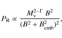
where the parameter ![]() is defined by
is defined by
![]() (
(
![]() in the virial scaling). Equation (3) implies that more massive clusters host more luminous radio halos. By considering halos with
in the virial scaling). Equation (3) implies that more massive clusters host more luminous radio halos. By considering halos with
![]() GHz, C06 showed that the slope of this scaling is consistent with that of the observed
GHz, C06 showed that the slope of this scaling is consistent with that of the observed
![]() correlation, provided that the model parameters
correlation, provided that the model parameters
![]() lie
within a fairly constrained range of values (see Fig. 7 in C06).
We refer the reader to Sects. 3.3 and 4.1 of C06 for a more
detailed discussion on model parameters and their constraints.
lie
within a fairly constrained range of values (see Fig. 7 in C06).
We refer the reader to Sects. 3.3 and 4.1 of C06 for a more
detailed discussion on model parameters and their constraints.
Following C09, we adopt a reference set of parameters![]() :
:
![]() G, b=1.5,
G, b=1.5,
![]() that falls in that range and sets
that falls in that range and sets
![]() ,
with
,
with
![]() .
This implies
.
This implies
![]() assuming the
assuming the
![]() correlation for galaxy clusters as derived in C06.
Because the bulk of radio halos in our calculations is found to be associated with clusters of mass
correlation for galaxy clusters as derived in C06.
Because the bulk of radio halos in our calculations is found to be associated with clusters of mass ![]()
![]() the adopted values of B and b imply typical average magnetic fields
the adopted values of B and b imply typical average magnetic fields ![]() 1-3
1-3 ![]() G. These values of B are similar to those derived from rotation measurements (e.g., Govoni & Feretti 2004; Bonafede et al. 2010) and equipartition assumption (Enßlin et al. 1998; Govoni et al. 2001).
G. These values of B are similar to those derived from rotation measurements (e.g., Govoni & Feretti 2004; Bonafede et al. 2010) and equipartition assumption (Enßlin et al. 1998; Govoni et al. 2001).
The observed
![]() correlation shows an intrinsic scatter across the radio luminosity
correlation shows an intrinsic scatter across the radio luminosity
![]() (e.g., Brunetti et al. 2009). In principle, in our model a scatter in the
(e.g., Brunetti et al. 2009). In principle, in our model a scatter in the
![]() correlation is expected due to the different monochromatic radio luminosity of halos with different
correlation is expected due to the different monochromatic radio luminosity of halos with different
![]() (Eq. (2)). Our calculations show that the fraction of clusters hosting radio halos with
(Eq. (2)). Our calculations show that the fraction of clusters hosting radio halos with
![]() MHz is about a few percent, thus we would expect
MHz is about a few percent, thus we would expect
![]() for halos with
for halos with
![]() GHz,
which agrees with the observed scatter. However, we stress that there
are other possible sources of scatter which are difficult to take into
account in homogeneous models. These are due to e.g., differences
in the cosmic rays and magnetic field content in clusters with the same
mass.
GHz,
which agrees with the observed scatter. However, we stress that there
are other possible sources of scatter which are difficult to take into
account in homogeneous models. These are due to e.g., differences
in the cosmic rays and magnetic field content in clusters with the same
mass.
Once we anchor the luminosity of halos with
![]() GHz,
GHz,
![]() ,
to the observed
,
to the observed
![]() correlation, Monte Carlo calculations carried out by considering an observing frequency
correlation, Monte Carlo calculations carried out by considering an observing frequency ![]() and Eq. (2)
allow us to derive the expected radio halo luminosity functions (RHLF;
see e.g., C06 & C09 for details). As an example, Fig. 1 shows the total RHLF obtained from Monte Carlo calculations at
and Eq. (2)
allow us to derive the expected radio halo luminosity functions (RHLF;
see e.g., C06 & C09 for details). As an example, Fig. 1 shows the total RHLF obtained from Monte Carlo calculations at ![]() MHz (black line) and z=0-0.1, together with the differential contributions to the RHLF from halos with different
MHz (black line) and z=0-0.1, together with the differential contributions to the RHLF from halos with different
![]() (see figure caption). As expected, radio halos with smaller
(see figure caption). As expected, radio halos with smaller
![]() mainly contribute to the low-power end of the total RHLF, and the peaks
of the RHLF of different populations move towards low radio powers with
decreasing
mainly contribute to the low-power end of the total RHLF, and the peaks
of the RHLF of different populations move towards low radio powers with
decreasing
![]() .
This implies that depending on their sensitivity, surveys at low radio frequency will unveil new populations of halos.
.
This implies that depending on their sensitivity, surveys at low radio frequency will unveil new populations of halos.
3 Monte Carlo distributions of radio halos in the P
 L
L plane
plane
The aim of this section is to investigate how the new population of
ultra-steep spectrum halos, predicted in deep low frequency radio
surveys, may affect the radio-X-ray luminosity correlation of halos at
low radio frequency. LOFAR will carry out surveys between 15 and
210 MHz in the Northern hemisphere with unprecedented sensitivity
and spatial resolution. Because LOFAR is expected to carry out the
deepest large area radio surveys at
![]() MHz (e.g., Röttgering et al. 2006), we focus here on the
MHz (e.g., Röttgering et al. 2006), we focus here on the
![]() correlation.
correlation.
![\begin{figure}
{
\includegraphics[width=8cm,clip]{13622f1.ps} }\end{figure}](/articles/aa/full_html/2010/09/aa13622-09/img76.png)
|
Figure 1:
Radio halo luminosity function at 120 MHz (black lines) and in the redshift interval z=0-0.1. The differential contributions from halos with
|
| Open with DEXTER | |
The most crucial point in this respect is the estimate of the minimum
diffuse flux of a radio halo detectable by these surveys as a function
of redshift. It is well known that the brightness profiles of radio
halos smoothly decreases with the distance from the cluster center
(e.g., Govoni et al. 2001; Murgia et al. 2009), implying that the outermost region of the halos will be difficult to detect in radio surveys.
Brunetti et al. (2007) found that the typical profiles of radio halos are such that about 58% of their flux is contained within the half radius (![]() ). Following C09 we assume a beam of
). Following C09 we assume a beam of
![]() arcsec to have a good sensitivity to diffuse emission and estimate the
minimum flux of a Mpc-sized halo detectable in a LOFAR survey,
arcsec to have a good sensitivity to diffuse emission and estimate the
minimum flux of a Mpc-sized halo detectable in a LOFAR survey, ![]() ,
by requiring that the mean brightness within the half radius of a halo,
,
by requiring that the mean brightness within the half radius of a halo,
![]() ,
is
,
is ![]() times the rms (F) of the survey, i.e.,
times the rms (F) of the survey, i.e.,
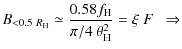
![$\displaystyle \quad f_{\rm H}(z)\simeq 2\times 10^{-3}\Big[\frac{\xi ~ F}{{\rm mJy/b}}\Big]~](/articles/aa/full_html/2010/09/aa13622-09/img83.png)
where
![]() is the angular size of radio halos in arcseconds at a given redshift.
For
is the angular size of radio halos in arcseconds at a given redshift.
For
![]() this approach would guarantee the detection at several
this approach would guarantee the detection at several ![]() of the central brightest region of halos, thus leading to the identification of candidate radio halos in the survey.
of the central brightest region of halos, thus leading to the identification of candidate radio halos in the survey.
This simple approach has been tested in Cassano et al. (2008) by injecting ``fake'' radio halos in the (u, v)
plane of NVSS and GMRT observations. It has been shown that radio halos
become visible in the images as soon as their flux approaches that
obtained by Eq. (4) with ![]() and
and ![]() for the NVSS and GMRT observations, respectively (see also Brunetti et al. 2007; Venturi et al. 2008).
for the NVSS and GMRT observations, respectively (see also Brunetti et al. 2007; Venturi et al. 2008).
![\begin{figure}
\par\mbox{\includegraphics[width=6cm]{13622f2a.ps}\includegraphics[width=6cm]{13622f2b.ps}\includegraphics[width=6cm]{13622f2c.ps} }\end{figure}](/articles/aa/full_html/2010/09/aa13622-09/img90.png)
|
Figure 2:
Expected distribution of radio halos in the
|
| Open with DEXTER | |
![\begin{figure}
\par\mbox{\includegraphics[width=7.5cm]{13622f3a.ps}\includegraphics[width=7.5cm]{13622f3b.ps} }
\end{figure}](/articles/aa/full_html/2010/09/aa13622-09/img92.png)
|
Figure 3:
Radio-X-ray luminosity correlation of giant radio halos at
1.4 GHz. Observed halos at 1.4 GHz (black points) and
``simulated halos'' with
|
| Open with DEXTER | |
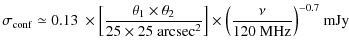
where
![]() is the beam size in arcsec, and
is the beam size in arcsec, and ![]() is the frequency in MHz.
is the frequency in MHz.
Of course all the issues discussed above will be clarified during the
commissioning phase of LOFAR. Thus we decided to present calculations
for several cases, specifically
![]() ,
0.6 and 1 mJy/beam to cover a range of possible LOFAR sensitivities
,
0.6 and 1 mJy/beam to cover a range of possible LOFAR sensitivities![]() .
Vertical dashed lines in Fig. 1 show the minimum power of a halo at
.
Vertical dashed lines in Fig. 1 show the minimum power of a halo at
![]() detectable by LOFAR surveys assuming
detectable by LOFAR surveys assuming
![]() and 1 mJy/beam. The important point is that with increasing survey
sensitivity new populations of radio halos are expected to be detected,
with the detectable number of ultra steep spectrum halos increasing in
deeper surveys.
and 1 mJy/beam. The important point is that with increasing survey
sensitivity new populations of radio halos are expected to be detected,
with the detectable number of ultra steep spectrum halos increasing in
deeper surveys.
The LOFAR observations will allow us to study the distribution
of radio halos in the radio-X-ray luminosity diagram at low radio
frequencies, so far an unexplored issue. The vast majority of
ultra-steep spectrum halos visible at low frequencies are expected to
be associated with galaxy clusters of intermediate X-ray luminosity,
![]() erg/s, and should be less luminous than radio halos that are presently
observed at GHz frequencies. This should affect the radio-X-ray
luminosity correlation of halos at low frequencies, which is expected
to be steeper and have a larger scatter than that at 1.4 GHz.
erg/s, and should be less luminous than radio halos that are presently
observed at GHz frequencies. This should affect the radio-X-ray
luminosity correlation of halos at low frequencies, which is expected
to be steeper and have a larger scatter than that at 1.4 GHz.
To address this issue quantitatively we assumed ![]() MHz,
and following C06 and C09 used Monte Carlo procedures based on the
extended Press & Schechter (1974; Lacey & Cole 1993) formalism to obtain i) the population of galaxy clusters, with their mass (and X-ray luminosity), in the redshift interval z=0-0.5, and ii) the population of radio halos, with their
MHz,
and following C06 and C09 used Monte Carlo procedures based on the
extended Press & Schechter (1974; Lacey & Cole 1993) formalism to obtain i) the population of galaxy clusters, with their mass (and X-ray luminosity), in the redshift interval z=0-0.5, and ii) the population of radio halos, with their
![]() ,
associated with these clusters. We used homogeneous models and the set
of model parameters given in the previous section. From these
simulations we extracted the population of radio halos that can be
detected by observations at
,
associated with these clusters. We used homogeneous models and the set
of model parameters given in the previous section. From these
simulations we extracted the population of radio halos that can be
detected by observations at ![]() MHz according to their radio luminosity and
MHz according to their radio luminosity and
![]() .
.
In particular, the luminosity at 120 MHz of radio halos with
![]() GHz in clusters with X-ray luminosity
GHz in clusters with X-ray luminosity ![]() is obtained from the
is obtained from the
![]() correlation, assuming a spectral index
correlation, assuming a spectral index
![]() and allowing for a random scatter
and allowing for a random scatter
![]() (see discussion in Sect. 2).
The luminosity at 120 MHz of radio halos with a given
(see discussion in Sect. 2).
The luminosity at 120 MHz of radio halos with a given
![]() is obtained according to Eq. (2). In particular, we calculated halo statistics by assuming the following frequency ranges:
is obtained according to Eq. (2). In particular, we calculated halo statistics by assuming the following frequency ranges:
![]() MHz, 240-600 MHz,
600-1400 MHz.
Equation (2) also implies that halos with
MHz, 240-600 MHz,
600-1400 MHz.
Equation (2) also implies that halos with
![]() should have radio luminosities at 120 MHz which may scatter by a factor
should have radio luminosities at 120 MHz which may scatter by a factor
![]() ,
which implies
,
which implies
![]() for the frequency bins we are considering.
Finally, we assumed the LOFAR sky coverage (the Northern hemisphere,
for the frequency bins we are considering.
Finally, we assumed the LOFAR sky coverage (the Northern hemisphere,
![]() ,
and high Galactic latitudes,
,
and high Galactic latitudes,
![]() )
and
)
and
![]() from Eq. (4).
from Eq. (4).
The resulting theoretical distribution of radio halos in the
![]() diagram is shown in Fig. 2, assuming
diagram is shown in Fig. 2, assuming
![]() and 0.25 mJy/beam (colored open dots; from left to right).
Different colored dots indicate halos with different values of
and 0.25 mJy/beam (colored open dots; from left to right).
Different colored dots indicate halos with different values of
![]() (the same color code used in Fig. 1).
Halos with different
(the same color code used in Fig. 1).
Halos with different
![]() fill different regions, with radio halos with lower
fill different regions, with radio halos with lower
![]() typically located in regions of lower radio luminosities.
The number of halos with lower
typically located in regions of lower radio luminosities.
The number of halos with lower
![]() increases with increasing survey sensitivity. In high-sensitivity
surveys these halos dominate the population and their presence affects
the overall shape of the correlation. The correlation at 120 MHz
is predicted to be more scattered and steeper than that observed at
1.4 GHz. A quantitative estimate of the steepening can be obtained
by repeating the Monte Carlo procedure described above many times and
by fitting the obtained halo distributions in the
increases with increasing survey sensitivity. In high-sensitivity
surveys these halos dominate the population and their presence affects
the overall shape of the correlation. The correlation at 120 MHz
is predicted to be more scattered and steeper than that observed at
1.4 GHz. A quantitative estimate of the steepening can be obtained
by repeating the Monte Carlo procedure described above many times and
by fitting the obtained halo distributions in the
![]() diagram.
Figure 4 shows a histogram of the slopes of the correlation obtained after 100 Monte Carlo runs for
diagram.
Figure 4 shows a histogram of the slopes of the correlation obtained after 100 Monte Carlo runs for
![]() mJy/beam.
The mean value of the slope is
mJy/beam.
The mean value of the slope is
![]() ,
while we find
,
while we find
![]() and 2.46 for
and 2.46 for
![]() and 0.6 mJy/beam, respectively (with 68% of values typically within
and 0.6 mJy/beam, respectively (with 68% of values typically within
![]() ). The values of
). The values of
![]() are significantly higher
than those at 1.4 GHz.
are significantly higher
than those at 1.4 GHz.
![\begin{figure}
\par {\includegraphics[width=8cm]{13622f4.ps} }\end{figure}](/articles/aa/full_html/2010/09/aa13622-09/img122.png)
|
Figure 4:
Spectral slopes of the
|
| Open with DEXTER | |
For completeness we show in Fig. 3 in the left panel, the theoretical distribution of giant radio halos with
![]() MHz (red points) in the
P(1400)-LX plane together with the observed correlation of halos at 1400 MHz (black points, taken from Brunetti et al. 2009;
see Table 1 and references therein).
Here we follow C09 (Sect. 3) to compare model expectations and
present observations and derive the theoretical distribution of radio
halos by considering the combination of the NVSS-XBACs (Giovannini
et al. 1999) (radio-X-ray) selection criteria and sky coverage (at
z=0.044-0.2), and the X-ray luminosity range and sky coverage of the GMRT radio halo survey (Venturi et al. 2007, 2008) (at
z=0.2-0.32)
MHz (red points) in the
P(1400)-LX plane together with the observed correlation of halos at 1400 MHz (black points, taken from Brunetti et al. 2009;
see Table 1 and references therein).
Here we follow C09 (Sect. 3) to compare model expectations and
present observations and derive the theoretical distribution of radio
halos by considering the combination of the NVSS-XBACs (Giovannini
et al. 1999) (radio-X-ray) selection criteria and sky coverage (at
z=0.044-0.2), and the X-ray luminosity range and sky coverage of the GMRT radio halo survey (Venturi et al. 2007, 2008) (at
z=0.2-0.32)![]() .
The observed and theoretical distributions agree well, although the
data points present a slightly larger scatter than expected, which can
be easily interpreted as due to variations of the magnetic field in
clusters with the same X-ray luminosity (see Sect. 2).
In Fig. 3, right panel,
the same observed distribution of radio halos at 1.4 GHz (black
points) is compared with that of ``simulated'' halos with
.
The observed and theoretical distributions agree well, although the
data points present a slightly larger scatter than expected, which can
be easily interpreted as due to variations of the magnetic field in
clusters with the same X-ray luminosity (see Sect. 2).
In Fig. 3, right panel,
the same observed distribution of radio halos at 1.4 GHz (black
points) is compared with that of ``simulated'' halos with
![]() MHz (red points) detectable by a LOFAR survey at 120 MHz with
MHz (red points) detectable by a LOFAR survey at 120 MHz with ![]() F = 0.25 mJy/beam. As expected, radio halos with
F = 0.25 mJy/beam. As expected, radio halos with
![]() GHz
follow a trend consistent with halos observed at present while their
larger number simply reflects the high sensitivity of LOFAR surveys
with respect to present surveys.
GHz
follow a trend consistent with halos observed at present while their
larger number simply reflects the high sensitivity of LOFAR surveys
with respect to present surveys.
3.1 Dependence on model parameters
The steepening of the correlation is independent of the adopted values
of model parameters, at least when considering sets of parameters in
the region (
![]() ,
b,
,
b,
![]() )
that reproduce both the observed slope of the
)
that reproduce both the observed slope of the
![]() correlation (
correlation (
![]() )
and the observed fraction of galaxy clusters with radio halos. Cassano
et al. (2006) and C09 already discussed the dependence of the
expectations on model parameters. They showed that the expected number
of radio halos decreases only by a factor of
)
and the observed fraction of galaxy clusters with radio halos. Cassano
et al. (2006) and C09 already discussed the dependence of the
expectations on model parameters. They showed that the expected number
of radio halos decreases only by a factor of ![]() 2-2.5, from super-linear (b>1) to sub-linear (b<1) magnetic scaling (see also Fig. 4 in Cassano et al. 2006).
2-2.5, from super-linear (b>1) to sub-linear (b<1) magnetic scaling (see also Fig. 4 in Cassano et al. 2006).
For a fixed value of b higher values of
![]() produce
produce
![]() correlations with slightly flatter slopes (see Table 3 in C06). For example, for b=1.5 the allowed values of B range from
correlations with slightly flatter slopes (see Table 3 in C06). For example, for b=1.5 the allowed values of B range from
![]() G to
G to
![]() G, and correspondingly it is
G, and correspondingly it is
![]() and 2.5, respectively, still consistent with the observed one.
and 2.5, respectively, still consistent with the observed one.
![\begin{figure}
\par {\includegraphics[width=8cm]{13622f5.ps} }\end{figure}](/articles/aa/full_html/2010/09/aa13622-09/img127.png)
|
Figure 5:
Fraction of clusters with radio halos with
|
| Open with DEXTER | |
![\begin{figure}
\par\includegraphics[width=6cm]{13622f6a.ps}\includegraphics[width=6cm]{13622f6b.ps}\includegraphics[width=6cm]{13622f6c.ps}
\end{figure}](/articles/aa/full_html/2010/09/aa13622-09/img128.png)
|
Figure 6:
Left panel: time-evolution of the ratio between
|
| Open with DEXTER | |
The steepening of the correlation is due to the emergence of new radio
halos at low frequency, thus another point is whether the fraction of
halos with lower
![]() (ultra steep spectrum halos) changes from super-linear to sub-linear cases. To investigate this effect we report in Fig. 5 the percentage of radio halos with
(ultra steep spectrum halos) changes from super-linear to sub-linear cases. To investigate this effect we report in Fig. 5 the percentage of radio halos with
![]() MHz (magenta lines) and
MHz (magenta lines) and
![]() MHz (blue lines) as a function of the cluster X-ray luminosity. In Fig. 5 we assume two configurations of parameters: the one used here (solid lines) and a sub-linear one (
MHz (blue lines) as a function of the cluster X-ray luminosity. In Fig. 5 we assume two configurations of parameters: the one used here (solid lines) and a sub-linear one (
![]() G, b=0.6,
G, b=0.6,
![]() ,
dashed lines). In both cases, the vast majority of radio halos hosted in clusters with
,
dashed lines). In both cases, the vast majority of radio halos hosted in clusters with
![]() erg/s has
erg/s has
![]() MHz, while halos with
MHz, while halos with
![]() MHz become dominant in more luminous clusters. On the other hand,
we find that the fraction of halos with
MHz become dominant in more luminous clusters. On the other hand,
we find that the fraction of halos with
![]() MHz is larger in the sub-linear case. This is because it is more difficult to generate radio halos with higher
MHz is larger in the sub-linear case. This is because it is more difficult to generate radio halos with higher
![]() for lower magnetic fields (provided that radiative losses are dominated
by the Inverse-Compton losses due to the CMB photons). We may conclude
that in sub-linear cases we expect the following main effects: i) the
for lower magnetic fields (provided that radiative losses are dominated
by the Inverse-Compton losses due to the CMB photons). We may conclude
that in sub-linear cases we expect the following main effects: i) the
![]() diagram should be less populated than that in super-linear cases (less halos are expected); ii) the
diagram should be less populated than that in super-linear cases (less halos are expected); ii) the
![]() correlation is expected to be flatter than that in super-linear cases (see Table 3 in C06); iii) the
correlation is expected to be flatter than that in super-linear cases (see Table 3 in C06); iii) the
![]() diagram should be even more dominated by ultra-steep spectrum halos,
making the steepening of the correlation at lower frequency even
stronger.
diagram should be even more dominated by ultra-steep spectrum halos,
making the steepening of the correlation at lower frequency even
stronger.
4 The effect of an evolving magnetic field
We applied a statistical model based on the turbulence-acceleration scenario (discussed and developed in Cassano & Brunetti 2005; C06; and C09) to derive the expected distribution of radio halos in the
![]() diagram.
The cosmological evolution of the magnetic field in this model is
accounted for by scaling the field with the cluster mass, as suggested
by cosmological MHD simulations (e.g., Dolag et al. 2002;
see also Sect. 2). On the other hand, our calculations do not
self-consistently follow turbulence and the amplification of magnetic
fields due to this turbulence. The main reason for that is that in the
turbulence acceleration scenario radio halos are generated and
disappear due to the acceleration and cooling of the emitting
particles, and these processes are much faster (
diagram.
The cosmological evolution of the magnetic field in this model is
accounted for by scaling the field with the cluster mass, as suggested
by cosmological MHD simulations (e.g., Dolag et al. 2002;
see also Sect. 2). On the other hand, our calculations do not
self-consistently follow turbulence and the amplification of magnetic
fields due to this turbulence. The main reason for that is that in the
turbulence acceleration scenario radio halos are generated and
disappear due to the acceleration and cooling of the emitting
particles, and these processes are much faster (![]() 0.1-0.2 Gyr) than the slow decay of the magnetic field in the ICM,
0.1-0.2 Gyr) than the slow decay of the magnetic field in the ICM, ![]() few Gyr (e.g., Brunetti et al. 2009). Moreover, although particle-acceleration is demonstrated to be connected with cluster mergers (e.g., Buote 2001; Govoni et al. 2004; Venturi et al. 2008),
several mechanisms/sources of magnetic field other than mergers-induced
amplification may significantly contribute to the magnetic field in the
ICM. Indeed, higher values of magnetic fields are measured in cooling
core clusters, which are not merging systems (e.g., Carilli &
Taylor 2002; Govoni 2006).
Although it is clear that a self-consistent treatment of turbulence,
particle acceleration and magnetic field evolution is mandatory and
deserves future theoretical efforts, we show in this section that the
results presented here are not substantially affected by the evolution
of the magnetic field when clusters become more relaxed after a merging
phase.
few Gyr (e.g., Brunetti et al. 2009). Moreover, although particle-acceleration is demonstrated to be connected with cluster mergers (e.g., Buote 2001; Govoni et al. 2004; Venturi et al. 2008),
several mechanisms/sources of magnetic field other than mergers-induced
amplification may significantly contribute to the magnetic field in the
ICM. Indeed, higher values of magnetic fields are measured in cooling
core clusters, which are not merging systems (e.g., Carilli &
Taylor 2002; Govoni 2006).
Although it is clear that a self-consistent treatment of turbulence,
particle acceleration and magnetic field evolution is mandatory and
deserves future theoretical efforts, we show in this section that the
results presented here are not substantially affected by the evolution
of the magnetic field when clusters become more relaxed after a merging
phase.
In order to investigate the effect of an evolving magnetic
field on our results, we consider the simulations of the generation and
decay of dynamo-active turbulence developed by Subramanian, Shukurov
& Haugen (2006, hereafter SSH06). They studied the decay phase of
an induced turbulent flow and magnetic field that follows a saturation
phase after the driving is switched off. They found that after the
exponential growth of the magnetic field a saturation phase follows,
the turbulent energy and the magnetic energy decay in a way that after
an eddy-turnover timescale the turbulent energy density is about half
of its saturation value, while the magnetic field strength is still at ![]() 90% of the saturation value (see Fig. 2 in SSH06).
By considering random motion with a typical initial speed v0 = 500 km s-1 and scale
90% of the saturation value (see Fig. 2 in SSH06).
By considering random motion with a typical initial speed v0 = 500 km s-1 and scale
![]() kpc, which are appropriate for cluster-merger driven turbulence, the eddy-turnover timescale is
kpc, which are appropriate for cluster-merger driven turbulence, the eddy-turnover timescale is
![]() Gyr. Because we are interested in the evolution of radio halos on timescales of
Gyr. Because we are interested in the evolution of radio halos on timescales of ![]() Gyr and the radiative lifetime of the emitting particle is of
Gyr and the radiative lifetime of the emitting particle is of ![]() 0.1-0.3 Gyr, we can estimate the variation of the frequency
0.1-0.3 Gyr, we can estimate the variation of the frequency
![]() as a function of time by adopting the classical formula
as a function of time by adopting the classical formula
![]() (see also Sect. 2). The ratio between
(see also Sect. 2). The ratio between
![]() for a time-dependent magnetic field and for a constant magnetic field is reported in Fig. 6 (left panel), where t0= 1.1 Gyr (because here we have considered a saturation phase of
for a time-dependent magnetic field and for a constant magnetic field is reported in Fig. 6 (left panel), where t0= 1.1 Gyr (because here we have considered a saturation phase of
![]() Gyr before the driving is switched off).
Gyr before the driving is switched off).
Substantial differences are found only for t>2 Gyr when the halo is expected to have already disappeared however (
![]() ,
with
,
with
![]() the turbulence energy density). The ratio between the steepening frequencies (Fig. 6, left panel) at
the turbulence energy density). The ratio between the steepening frequencies (Fig. 6, left panel) at ![]() gives an estimate of the error we can make by neglecting the time-evolution of the magnetic field, that is
gives an estimate of the error we can make by neglecting the time-evolution of the magnetic field, that is ![]()
![]() .
.
In the central panel of Fig. 6 we also report the time-evolution of the synchrotron spectra at different times (t=0.9,
1.1, 1.5, 1.8 and 2 Gyr, see figure caption) by assuming a
constant magnetic field (as in the adopted model, solid lines) and an
evolving magnetic field (as in SSH06, dashed lines). For ![]() Gyr the difference in the monochromatic radio luminosities is less then 10%. In addition, the right panel of Fig. 6
shows the evolution of the spectral index between 1.4 GHz and
330 MHz of these synchrotron spectra. Up to 1.2-1.3 Gyr the
difference in the spectral indeces is very small, less then 10%.
Gyr the difference in the monochromatic radio luminosities is less then 10%. In addition, the right panel of Fig. 6
shows the evolution of the spectral index between 1.4 GHz and
330 MHz of these synchrotron spectra. Up to 1.2-1.3 Gyr the
difference in the spectral indeces is very small, less then 10%.
5 Conclusions
The observed correlations between the halo radio power (at
1.4 GHz) and the cluster X-ray luminosity, mass, and temperature
and the observed connection between radio halos and cluster mergers
suggest a link between the gravitational process of cluster formation
and the generation of radio halos. Radio halos are likely generated
during cluster-cluster mergers where a fraction of the gravitational
energy dissipated is channelled into the acceleration of relativistic
particles. A crucial expectation of the turbulent re-acceleration
scenario, put forward to explain radio halos, is that the synchrotron
spectrum of halos is characterized by a cut-off at frequency
![]() with
with
![]() determined by the efficiency of the acceleration process.
This cut-off causes a bias, so that present radio observations at
determined by the efficiency of the acceleration process.
This cut-off causes a bias, so that present radio observations at ![]() GHz
frequencies are expected to detect only the most efficient radio
phenomena in clusters, leaving unexplored a large population of radio
halos characterized by a spectral cut-off at lower frequencies
(e.g., C06; Brunetti et al. 2008;
C09). Future low-frequency radiotelescopes such as LOFAR and LWA are
expected to discover the populations of ultra steep spectrum radio
halos with
GHz
frequencies are expected to detect only the most efficient radio
phenomena in clusters, leaving unexplored a large population of radio
halos characterized by a spectral cut-off at lower frequencies
(e.g., C06; Brunetti et al. 2008;
C09). Future low-frequency radiotelescopes such as LOFAR and LWA are
expected to discover the populations of ultra steep spectrum radio
halos with
![]() GHz, which will enable us to test the idea of turbulent re-acceleration.
GHz, which will enable us to test the idea of turbulent re-acceleration.
One may wonder whether halos with
![]() GHz could be detected by present radiotelescopes at 1.4 GHz. To address this point we report in Fig. 7 the flux distribution at 1.4 GHz of halos with
GHz could be detected by present radiotelescopes at 1.4 GHz. To address this point we report in Fig. 7 the flux distribution at 1.4 GHz of halos with
![]() MHz (which in our model have
MHz (which in our model have
![]() between 120 MHz and 1400 MHz), which are expected to be detected by LOFAR at 120 MHz assuming
between 120 MHz and 1400 MHz), which are expected to be detected by LOFAR at 120 MHz assuming
![]() mJy/beam. Calculations are derived by assuming i) at z<0.3 the X-ray flux limit and sky coverage of the extended ROSAT Brightest Cluster Sample (eBCS, Ebeling et al. 1998, 2000) and of the ROSAT-ESO Flux Limited X-ray Galaxy Cluster Survey (REFLEX, Böringher et al. 2004), and ii) at
z=0.3-0.6 the X-ray flux limit and sky coverage of the Massive Cluster Survey (MACS, Ebeling et al. 2001).
Calculations show that potentially very deep pointed observations at
1.4 GHz of all these clusters may lead to the detection of a few
of these ultra steep spectrum halos (those with
mJy/beam. Calculations are derived by assuming i) at z<0.3 the X-ray flux limit and sky coverage of the extended ROSAT Brightest Cluster Sample (eBCS, Ebeling et al. 1998, 2000) and of the ROSAT-ESO Flux Limited X-ray Galaxy Cluster Survey (REFLEX, Böringher et al. 2004), and ii) at
z=0.3-0.6 the X-ray flux limit and sky coverage of the Massive Cluster Survey (MACS, Ebeling et al. 2001).
Calculations show that potentially very deep pointed observations at
1.4 GHz of all these clusters may lead to the detection of a few
of these ultra steep spectrum halos (those with
![]() MHz); the ultra steep spectrum halo detected in the cluster Abell 521 (Brunetti et al. 2008;
Dallacasa et al. 2009) belongs to this class of halos, although it
is among the flatter spectrum objects in this class, with
MHz); the ultra steep spectrum halo detected in the cluster Abell 521 (Brunetti et al. 2008;
Dallacasa et al. 2009) belongs to this class of halos, although it
is among the flatter spectrum objects in this class, with
![]() MHz.
MHz.
We discussed the consequence of this new population of radio halos on
the slope of the radio-X-ray luminosity correlation at low frequency.
According to homogeneous models, ultra-steep spectrum halos are
expected to be less luminous than halos with higher
![]() associated with clusters of the same mass. Also, radio halos with lower
associated with clusters of the same mass. Also, radio halos with lower
![]() should statistically be generated in clusters with smaller mass (and
should statistically be generated in clusters with smaller mass (and ![]() ).
The combination of these two expectations implies that the radio-X-ray
luminosity correlation should be broader and steeper at lower
frequencies.
).
The combination of these two expectations implies that the radio-X-ray
luminosity correlation should be broader and steeper at lower
frequencies.
![\begin{figure}
{
\par\includegraphics[width=8cm]{13622f7.ps} }
\par\end{figure}](/articles/aa/full_html/2010/09/aa13622-09/img147.png)
|
Figure 7:
Integrated number counts at 1.4 GHz of halos with
|
| Open with DEXTER | |
Based on this model, we performed Monte Carlo simulations of the distribution of radio halos in the
![]() plane.
We found that halos distribute in the
plane.
We found that halos distribute in the
![]() plane according to a correlation which is steeper (
plane according to a correlation which is steeper (
![]() )
and broader than that observed at 1.4 GHz, with ultra-steep
spectrum halos broadening the scatter in the region of low luminosity.
We found that the number of ultra-steep spectrum halos increases with
increasing survey sensitivity, and this further steepens the
correlation.
The forthcoming LOFAR surveys should constrain the expected steepening
of the correlation and test our expectations.
)
and broader than that observed at 1.4 GHz, with ultra-steep
spectrum halos broadening the scatter in the region of low luminosity.
We found that the number of ultra-steep spectrum halos increases with
increasing survey sensitivity, and this further steepens the
correlation.
The forthcoming LOFAR surveys should constrain the expected steepening
of the correlation and test our expectations.
Although a self-consistent treatment of turbulence acceleration and amplification of the magnetic field in clusters is mandatory and deserves future efforts, we show that the main components in the adopted scenario are two ``fast'' processes: particle acceleration and particle cooling that follows the decay of turbulence. Because this is a ``slow'' process, we show that the possible decay of the field with turbulence is not expected to significantly affect the modeling of halo statistics.
AcknowledgementsThis work is partially supported by grants PRIN-INAF 2007, PRIN-INAF 2008 and ASI-INAF I/088/06/0. R.C. thanks the anonymous referees for comments and suggestions, and G. Brunetti, M. Brüggen, H. J. A. Röttgering and T. Venturi for useful comments.
References
- Bacchi, M., Feretti, L., Giovannini, G., & Govoni, F. 2003, A&A, 400, 465 [NASA ADS] [CrossRef] [EDP Sciences] [Google Scholar]
- Blasi, P., & Colafrancesco, S. 1999, APh, 12, 169 [NASA ADS] [Google Scholar]
- Böhringer, H., Schuecker, P., Guzzo, L., et al. 2004, A&A, 425, 367 [NASA ADS] [CrossRef] [EDP Sciences] [Google Scholar]
- Bonafede, A., Feretti, L., Murgia, M., et al. 2010, A&A, 513, A30 [NASA ADS] [CrossRef] [EDP Sciences] [Google Scholar]
- Brunetti, G., & Lazarian, A. 2007, MNRAS, 378, 245 [NASA ADS] [CrossRef] [Google Scholar]
- Brunetti, G., Setti, G., Feretti, L., & Giovannini, G. 2001, MNRAS, 320, 365 [NASA ADS] [CrossRef] [Google Scholar]
- Brunetti, G., Venturi, T., Dallacasa, D., et al. 2007, ApJ, 670, L5 [NASA ADS] [CrossRef] [Google Scholar]
- Brunetti, G., Giacintucci, S., Cassano, R., et al. 2008, Nature, 455, 944 [NASA ADS] [CrossRef] [Google Scholar]
- Brunetti, G., Cassano, R., Dolag, K., & Setti, G. 2009, A&A, 507, 661 [NASA ADS] [CrossRef] [EDP Sciences] [Google Scholar]
- Brüggen, M., Ruszkowski, M., & Simionescu, A. 2005, ApJ, 631, L21 [NASA ADS] [CrossRef] [Google Scholar]
- Buote, D. A. 2001, ApJ, 553, 15 [Google Scholar]
- Carilli, C. L., & Taylor, G. B. 2002, ARA&A, 40, 319 [NASA ADS] [CrossRef] [Google Scholar]
- Cassano, R, 2009, in The Low-Frequency Radio Universe, ed. D. J. Saikia, D. A. Green, Y. Gupta, & T. Venturi (San Francisco: ASP), ASP Conf. Ser., 407, 223 [Google Scholar]
- Cassano, R., & Brunetti, G. 2005, MNRAS, 357, 1313 [NASA ADS] [CrossRef] [Google Scholar]
- Cassano, R., Brunetti, G., & Setti, G. 2006a, MNRAS, 369, 1577 (C06) [NASA ADS] [CrossRef] [Google Scholar]
- Cassano, R., Brunetti, G., & Setti, G. 2006b, Astron. Nachr., 327, 557 [NASA ADS] [CrossRef] [Google Scholar]
- Cassano R., Brunetti G., Setti G., et al. 2007, MNRAS, 378, 1565 [NASA ADS] [CrossRef] [Google Scholar]
- Cassano, R., Brunetti, G., Venturi, T., et al. 2008, A&A, 480, 687 [NASA ADS] [CrossRef] [EDP Sciences] [Google Scholar]
- Cassano, R., Brunetti, G., Rottgering, H. J. A., & Bruggen M. 2010, A&A, 509, 68 [Google Scholar]
- Clarke, T. E. 2005, ASP Conf. Ser., 345, 227 [NASA ADS] [Google Scholar]
- Condon, J. J. 1987, in Proceedings of the Arecibo Upgrading Workshop, ed. J. H. Taylor, & M. M. Davis (Arecibo: NAIC), 89 [Google Scholar]
- Dallacasa, D., Brunetti, G., Giacintucci, S., et al. 2009, ApJ, 699, 1288 [NASA ADS] [CrossRef] [Google Scholar]
- Dolag, K., Bartelmann, M., & Lesch, H. 2002, A&A, 387, 383 [NASA ADS] [CrossRef] [EDP Sciences] [Google Scholar]
- Dolag, K., Grasso, D., Springel, V., & Tkachev, I. 2005, JCAP, 1, 9 [Google Scholar]
- Dennison, B. 1980, ApJ, 239, L93 [NASA ADS] [CrossRef] [Google Scholar]
- Ebeling, H., Edge, A. C., Böhringer, H., et al. 1998, MNRAS, 301, 881 [NASA ADS] [CrossRef] [Google Scholar]
- Ebeling, H., Edge, A. C., Allen, S. W., et al. 2000, MNRAS, 318, 333 [NASA ADS] [CrossRef] [Google Scholar]
- Ebeling, H., Edge, A. C., & Henry, J. P. 2001, ApJ, 553, 668 [Google Scholar]
- Ensslin, T. A., Biermann, P. L., Klein, U., & Kohle, S. 1998, A&A, 332, 395 [NASA ADS] [Google Scholar]
- Enßlin, T. A., & Röttgering, H. 2002, A&A, 396, 83 [NASA ADS] [CrossRef] [EDP Sciences] [Google Scholar]
- Feretti, L. 2005, in X-Ray and Radio Connections, published electronically by NRAO, ed. L. O. Sjouwerman, & K. K. Dyer [Google Scholar]
- Ferrari, F., Govoni, F., Schindler, S., et al. 2008, SSRv, 134, 93 [Google Scholar]
- Fujita, Y., Takizawa, M., & Sarazin, C. L. 2003, ApJ, 584, 190 [NASA ADS] [CrossRef] [Google Scholar]
- Giacintucci, S., Venturi, T., Brunetti, G., et al. 2009, A&A, 505, 45 [NASA ADS] [CrossRef] [EDP Sciences] [Google Scholar]
- Giovannini, G., Tordi, M., & Feretti, L. 1999, NewA, 4, 141 [Google Scholar]
- Giovannini, G., Bonafede, A., Feretti, L. 2009, A&A, 507, 1257 [NASA ADS] [CrossRef] [EDP Sciences] [Google Scholar]
- Govoni, F. 2006, Astron. Nachr., 327, 539 [Google Scholar]
- Govoni, F., & Feretti, L. 2004, Int. J. Mod. Phys. D, 13, 1549 [NASA ADS] [CrossRef] [Google Scholar]
- Govoni, F., Feretti, L., Giovannini, G., et al. 2001, A&A, 376, 803 [NASA ADS] [CrossRef] [EDP Sciences] [Google Scholar]
- Govoni, F., Markevitch, M., & Vikhlinin, A. 2004, ApJ, 605, 695 [NASA ADS] [CrossRef] [Google Scholar]
- Hoeft, M., & Brüggen, M. 2007, MNRAS, 375, 77 [NASA ADS] [CrossRef] [Google Scholar]
- Kempner, J. C., & Sarazin, C. L. 2001, ApJ, 548, 639 [NASA ADS] [CrossRef] [Google Scholar]
- Kronberg, P. P., Kothes, R., Salter, C. J., & Perillat, P. 2007, ApJ, 659, 267 [NASA ADS] [CrossRef] [Google Scholar]
- Lacey, C., & Cole, S. 1993, MNRAS, 262, 627 [NASA ADS] [CrossRef] [Google Scholar]
- Liang, H., Hunstead, R. W., Birkinshaw, M., & Andreani, P. 2000, ApJ, 544, 686 [NASA ADS] [CrossRef] [Google Scholar]
- Murgia, M., Govoni, F., Markevitch, M., et al. 2009, A&A, 499, 679 [NASA ADS] [CrossRef] [EDP Sciences] [Google Scholar]
- Petrosian, V. 2001, ApJ, 557, 560 [NASA ADS] [CrossRef] [Google Scholar]
- Pfrommer, C., & Enßlin, T. A. 2004, A&A, 413, 17 [NASA ADS] [CrossRef] [EDP Sciences] [Google Scholar]
- Pfrommer, C., Enßlin, T. A., & Springel V. 2008, MNRAS, 385, 1211 [NASA ADS] [CrossRef] [Google Scholar]
- Press, W. H., & Schechter, P. 1974, ApJ, 187, 425 [NASA ADS] [CrossRef] [Google Scholar]
- Röttgering, H. J. A., Braun, R., Barthel, P. D., et al. 2006, [arXiv:0610596] [Google Scholar]
- Rudnick, L., & Lemmerman, J. A. 2009, ApJ, 697, 1341 [NASA ADS] [CrossRef] [Google Scholar]
- Ryu, D., Kang, H., Cho, J., & Das, S. 2008, Science, 320, 909 [NASA ADS] [CrossRef] [PubMed] [Google Scholar]
- Schuecker, P., Böhringer, H., Reiprich, T. H., et al. A&A, 378, 408 [Google Scholar]
- Subramanian, K., Shukurov, A., Haugen, N. E. L. 2006, MNRAS, 366, 1437 [NASA ADS] [CrossRef] [Google Scholar]
- Vazza, F., Brunetti, G., & Kritsuk, A. 2009, A&A, 504, 33 [NASA ADS] [CrossRef] [EDP Sciences] [Google Scholar]
- Venturi, T., Giacintucci, S., Brunetti, G., et al. 2007, A&A, 463, 937 [NASA ADS] [CrossRef] [EDP Sciences] [Google Scholar]
- Venturi, T., Giacintucci, S., Dallacasa, et al. 2008, A&A, 484, 327 [NASA ADS] [CrossRef] [EDP Sciences] [Google Scholar]
Footnotes
- ...

![[*]](/icons/foot_motif.png)
-
 is the value of the magnetic field averaged in a region of radius =
500 h50-1 kpc in a cluster with viral mass
is the value of the magnetic field averaged in a region of radius =
500 h50-1 kpc in a cluster with viral mass
 .
.
- ... parameters
- We note that for this particular configuration of parameters even for the re-acceleration phase the energy of magnetic field is always dominant with respect to that of relativistic electrons.
- ... sensitivities
- Note that our choice of
 is thought to mimic different possible configurations, e.g.,
 mJy/beam can be
  (3
(3 detection of the average halo brightness in half
  )
and F = 0.2 mJy/beam, or
)
and F = 0.2 mJy/beam, or  and F = 0.6 mJy/beam.
- ...
z=0.2-0.32)
- The bulk of halos is found in these surveys.
All Figures
|
|
Figure 1:
Radio halo luminosity function at 120 MHz (black lines) and in the redshift interval z=0-0.1. The differential contributions from halos with
|
| Open with DEXTER | |
| In the text | |
|
|
Figure 2:
Expected distribution of radio halos in the
|
| Open with DEXTER | |
| In the text | |
|
|
Figure 3:
Radio-X-ray luminosity correlation of giant radio halos at
1.4 GHz. Observed halos at 1.4 GHz (black points) and
``simulated halos'' with
|
| Open with DEXTER | |
| In the text | |
|
|
Figure 4:
Spectral slopes of the
|
| Open with DEXTER | |
| In the text | |
|
|
Figure 5:
Fraction of clusters with radio halos with
|
| Open with DEXTER | |
| In the text | |
|
|
Figure 6:
Left panel: time-evolution of the ratio between
|
| Open with DEXTER | |
| In the text | |
|
|
Figure 7:
Integrated number counts at 1.4 GHz of halos with
|
| Open with DEXTER | |
| In the text | |
Copyright ESO 2010
Current usage metrics show cumulative count of Article Views (full-text article views including HTML views, PDF and ePub downloads, according to the available data) and Abstracts Views on Vision4Press platform.
Data correspond to usage on the plateform after 2015. The current usage metrics is available 48-96 hours after online publication and is updated daily on week days.
Initial download of the metrics may take a while.