| Issue |
A&A
Volume 517, July 2010
|
|
|---|---|---|
| Article Number | A1 | |
| Number of page(s) | 27 | |
| Section | Interstellar and circumstellar matter | |
| DOI | https://doi.org/10.1051/0004-6361/200811159 | |
| Published online | 23 July 2010 | |
Complex molecule formation in grain
mantles![[*]](/icons/foot_motif.png)
P. Hall1,2 - T. J. Millar3
1 - Department of Physics, UMIST, PO Box 88, Manchester, M60 1QD, UK
2 - Astronomy Department, Cornell University, Ithaca, New York,
14853-6801, USA
3 - Astrophysics Research Centre, School of Mathematics and Physics,
Queen's University, Belfast, BT7 1NN, Northern Ireland
Received 15 October 2008 / Accepted 26 March 2010
Abstract
Context. Complex molecules such as ethanol and
dimethyl ether have been observed in a number of hot molecular cores
and hot corinos. Attempts to model the molecular formation process
using gas phase only models have so far been unsuccessful.
Aims. To demonstrate that grain surface processing
is a viable mechanism for complex molecule formation in these
environments.
Methods. A variable environment parameter computer
model has been constructed which includes both gas and surface
chemistry. This is used to investigate a variety of cloud collapse
scenarios.
Results. Comparison between model results and
observation shows that by combining grain surface processing with gas
phase chemistry complex molecules can be produced in observed
abundances in a number of core and corino scenarios. Differences in
abundances are due to the initial atomic and molecular composition of
the core/corino and varying collapse timescales.
Conclusions. Grain surface processing, combined with
variation of physical conditions, can be regarded as a viable method
for the formation of complex molecules in the environment found in the
vicinity of a hot core/corino and produce abundances comparable to
those observed.
Key words: stars: formation - ISM: molecules - ISM: abundances - astrochemistry
1 Introduction
A number of complex molecules have been discovered in the interstellar medium. First was methanol, CH3OH, (Ball 1970) followed by dimethyl ether, CH3OCH3, (Snyder et al. 1974) and ethanol, CH3CH2OH, (herein denoted C2H5OH) (Zuckerman et al. 1975). A variety of other isomers, isotopic variants and similar compounds have also been seen. Charnley et al. (1995) review the distribution of complex molecules while Ikeda et al. (2001 & 2002) present more recent observations. CH3OH is seen in cold dark clouds with a relative abundance of 10-9 (with respect to H2) while in hot cores this can be as large as 10-6. The highest abundances are observed in regions where grain mantles are likely to have recently evaporated, strongly suggesting mantle processing either directly or in the formation of precursors.
A variety of computer models have been constructed to investigate molecule formation. Predominantly these are based on chemical reaction networks and use a flat (fixed) parameter space. As with the models presented here most are single point, where a single representative point in a cloud is modelled. This is satisfactory as chemistry at another point with different physical parameters could be modelled simply by changing the parameters. Over time the size and complexity of the reaction networks has increased as more reaction rate data is published in the literature and greater computer power becomes available to process more complex networks. (See Millar 1990, for a review of model development.) Millar et al. (1991b) model the production of CH3OH by a fixed parameter gas-phase-only model and are unable to produce abundances in excess of 10-7 lending further weight to the involvement of grain mantle processing. C2H5OH is seen in fewer sources than CH3OH and all known sources are dense, hot core star-forming regions, exactly the places where grain mantles are likely to evaporate. Abundances are in the range 10 -9-10-8 (with respect to H2). CH3OCH3 is often seen in the same sources as C2H5OH and has recently been detected in hot corinos (Ceccarelli et al. 2004; Bottinelli et al. 2004). It has an abundance range of 10 -8-10-6and the CH3OCH3/C2H5OH abundance ratio differs greatly between apparently similar sources. (Abundances with respect to H2 for selected sources are listed in Table 1.)
Table 1: Observed fractional abundances of complex molecules.
Even under very favorable conditions fixed parameter gas-phase-only chemical models produce maximum abundances for C2H5OH and CH3OCH3 of the order of 10-11(Herbst & Leung 1989; Millar et al. 1991a; Charnley et al. 1992), between two and five orders of magnitude below that observed. Again this suggests a scenario in which mantles form on dust grains at some point in a cloud's lifetime when conditions are favorable. The mantles are active and complex molecules (or their precursors) form on them more efficiently than in the gas phase. Later the cloud evolves becoming warmer and denser and the contents of the mantles pass back into the gas phase. Several other gas-phase-only models (for example Charnley et al. 1992; Caselli et al. 1993) have demonstrated that the chemistry in hot cores is active, with particular gas phase reaction channels initiated with simple species thought to originate from mantles, a possible explanation for observed complex molecule abundances.
A number of more in-depth models have included surface reaction chemistry. One of the first has been developed by Hasegawa et al. (1992) and Hasegawa & Herbst (1993). This model has 274 chemical species with 2928 reactions and includes 1% (by mass) dust grains in the gas cloud. Molecules can freeze out onto grains and later pass back into the gas phase. Once on a grain heavier species molecules are held stationary at lattice binding sites while lighter species, most commonly hydrogen atoms, can migrate around the grain. When mobile light species encounter fixed heavy species the two can combine to produce progressively larger molecules. While large molecules can evaporate off the grain surface there are a number of other possible desorbtion mechanisms that can act as well. (See Sect. 2.3.) One additional benefit of this approach is that grain surface catalysis of hydrogen molecules can be modelled directly.
Shalabiea & Greenberg (1995) then take the next logical step in interstellar cloud modelling by including variations in physical parameters. They use a gas phase reaction rate network and interchange between gas and surface similar to Hasegawa et al. (1992) and Hasegawa & Herbst (1993). However certain physical parameters (eg. density) can also change. Shalabiea & Greenberg (1995) model these by including differential equations for them and solving for the relevant parameter(s) at each point in time in much the same way as species abundances are solved for. They also coin the terms pseudo-time-dependent, where the model chemistry evolves over time while the parameters are static and real-time-dependent where both chemistry and physical parameters evolve. Their paper provides comparison between the two types, with the gas and grain model including 218 chemical species and 2075 reactions. With the more recent identification of hot corinos (Table 1 and Sect. 3.1) where the temperature range is optimal for the grain surface production of larger molecules and their subsequent return to the gas phase some specific modelling of these type of objects has been done. Garrod & Herbst (2006) use a gas and grain reaction network with 655 species and 6509 reactions. The same model was used by Aikawa et al. (2008). Subsequently Garrod et al. (2008) produced an extended and more generalized version. Comparison of the output of these models with the results presented here is made in Sect. 5.
As is discussed further in Sect. 2.3 some mechanism(s) must be returning material from grain mantles back to the gas phase since the alternative is depletion of molecular species heavier than H2 in a timescale shorter than the lifetime of known clouds, which is not seen. More recent modelling work has focused on the investigating the effectiveness of several proposed desorption mechanisms. Willacy & Millar (1998) provide a set of gas and surface models which include different desorption mechanisms and compare their effectiveness. These models use 282 species and 4864 reactions. Garrod et al. (2007) specifically model formation of CH3OH in a quiescent cloud and point out that if grain surface processes are invoked to explain the abundance of CH3OH then at least one non-thermal desorbtion mechanism must be active. Tielens & Charnley (1997) have argued that, at least in some cases, the reaction network model cannot be justified and that a Monte Carlo simulation approach is more appropriate. This has led to some debate in the current literature about the relative merits of the two methods. Willacy & Millar (1998) discuss this and conclude that currently there are computational impracticalities in using the Monte Carlo approach in real-time-dependent models, and further that the two different approaches may give fairly similar results for systems of increasing complexity. A direct comparison of the two approaches by Garrod et al. (2009) demonstrates considerable similarity between them. Certainly previous gas phase only reaction rate models have yielded results comparable with observations for many species.
The model used here builds on its predecessors. Termed the Gas/Surface model it is a single point, gas and surface phase, chemical reaction network model with 279 species and 2968 reactions. It includes the grain surface mechainsm used by Hasegawa et al. (1992) and Hasegawa & Herbst (1993) as well as the desorption mechanisms discussed by Willacy & Millar (1998). It is also fully real-time-dependent. Instead of the differential equation approach taken by Shalabiea & Greenberg (1995) each separate time step has its own set of physical parameters which are fed into the model from a storage file at the beginning of each time step. This approach has several advantages. Firstly it reduces computational strain on the model since there is no additional equation solving necessary. This is particularly important in situations where parameters are changing very quickly and there are major differences between adjacent time steps. (For example in the final stages of a cloud collapse where density increases drastically in a short time.) Secondly, this approach allows the same set of software to be used to model multiple different situations with no reprogramming at all. Only the input parameter file has to be changed. This allows great flexibility in the scope of scenarios that could be investigated. Further, in certain situations where there are major, abrupt changes in physical parameters (eg. shocks), the differential equation approach is highly prone to breakdown as generating a numerical solution for a given parameter requires some level of continuity between one time step and the next, wheras the parameter file approach avoids this problem completely.
The Gas/Surface model is used here to investigate the scenario of complex molecule formation in grain mantles and their subsequent release back into the gas phase. We consider clouds at a variety of initial densities with different exposure to photoionization. As these clouds collapse to become denser and darker, their chemistry becomes more complex and their temperature drops allowing grain mantles to form. Simple gas-phase dominated chemistry at the beginning leads to the deposition of a variety of basic molecules onto an initially bare grain surface. Once on the grain, surface processes allow the build up of complex molecules in a frozen mantle. Later, as the cloud heats up, the mantle evaporates introducing the complex molecules into the gas phase with a variety of chemical consequences significantly different from gas phase only processing.
2 The Gas/Surface model
2.1 Design of the model
The Gas/Surface model is used here to model a collapse situation. A cloud collapse begins with the cloud optically thin and open to heating by external photons. Self shielding of H2 is treated by the method of Wagenblast (1992). As it contracts it eventually becomes optically thick to external photons and its inner regions cool. It is this cooling which allows molecules to freeze out onto dust grain surfaces and form mantles. Eventually continuing collapse of the cloud, assisted possibly by the ignition of a proto-star at its center, causes the temperature to rise again desorping the mantles off the grain and returning mantle processed species to the gas phase. The model allows interchange between gas and surface phases, both freezing, thermal desorption and a variety of other continously acting desorbtion mechanisms, as described by Willacy (1993) and Willacy & Millar (1998). (See Sect. 2.3.) Once on the grain surface chemistry takes place as described in Sect. 2.2.
The reaction networks are solved numerically using the GEAR package (Hindmarsh 1974, 1983). It is the combination of both a time variable parameter space and interchange between gas and surface phase chemistry that makes the Gas/Surface model appropriate to investigate complex molecule formation. A fuller description of the model design can be found in Hall (1997).
2.2 Surface chemistry mechanism
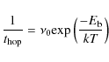
The surface chemistry mechanism used in the Gas/Surface model is taken from Hasegawa et al. (1992) and Hasegawa & Herbst (1993) with additional complex molecule formation reactions listed in the Appendix. Surface species are prefixed * to distinguish them from their gas phase counterparts. This scheme allows fourteen low molecular mass species (Table 2) to be mobile on the grain surface while all other surface species are stationary, held at sites on the surface. The adsorption energy ED (in K) is the energy needed to liberate the species from the grain surface back into the gas phase. Parameter values (and their references) are listed in Table 4.
The mobile species migrate around the grain surface
by hopping from site to site.
A mobile species arriving at an occupied site
can react with either a stationary species already there or another
mobile species which has also just arrived.
Mobile species are regarded as occupying any given site for a finite
period of time, generally about 10-12 s,
the exact time being determined
by species mass and prevailing temperature.
There is an energy potential barrier separating adjacent sites and
mobile species must possess sufficient energy to overcome it. For most
of the mobile species classical type motions only are permitted. The
species must have sufficient classical kinetic energy to cross
potential barriers.
For atomic and molecular hydrogen however quantum tunnelling through
barriers is permitted.
Which reactions take place is governed by a reaction set
(Sect. 2.4)
analogous to those used for gas phase reactions, each with an
accompanying rate coefficient.
The grain itself is assumed to be inert and all surface chemistry
involves the mantle only.
The classical mobile species migrate over the grain surface.
The time to move
between two adjacent surface sites (hopping time)
![]() is
given by:
is
given by:
|
(1) |
where T is the grain surface temperature and

|
(2) |
Table 2: Mobile surface species.
where ![]() is the surface density of sites (
is the surface density of sites (![]()
![]() m-2)
and m is the mass of the mobile species (in kg).
This gives values of
m-2)
and m is the mass of the mobile species (in kg).
This gives values of ![]() in the range 10
12-1013 s-1.
Hydrogen atoms and molecules are held to be quantum particles and their
hopping times are given by the time for them to quantum tunnel
through the potential barrier:
in the range 10
12-1013 s-1.
Hydrogen atoms and molecules are held to be quantum particles and their
hopping times are given by the time for them to quantum tunnel
through the potential barrier:
![\begin{displaymath}\frac{1}{t_{\rm hop}} = \nu_{0} {\rm exp}
\left[ \frac{-2a}{\hbar} \sqrt{2mE_{\rm b}}
\right]
\end{displaymath}](/articles/aa/full_html/2010/09/aa11159-08/img27.png)
|
(3) |
where a is the separation between two adjacent sites (

|
(4) |
where
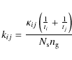
|
(5) |
where ti and tj are the hopping times for species i and j and
|
(6) |
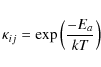
In the quantum case where at least one of the reactants is a hydrogen atom or molecule:
![\begin{displaymath}\kappa_{ij} = {\rm exp} \left[\frac{-2a}{\hbar} \sqrt{2\mu E_a}\right]
\end{displaymath}](/articles/aa/full_html/2010/09/aa11159-08/img38.png)
|
(7) |
where
2.3 Desorption mechanisms
Desorption mechanisms can be divided into two basic classes, continuously acting which remove a few atoms/molecules at any one time and irregular such as shocks, which occur at random intervals but return most or all of a grain mantle to the gas phase. In the scenarios modelled here there are no shocks or similar mechanisms of sufficient strength to desorb mantles and continous mechanisms dominate. Willacy (1993) provides an in-depth treatment of continuous mechanisms and four of them have been included in the models presented here:
- 1.
- Mantle Explosion;
- 2.
- Direct UV Photodesorption;
- 3.
- Cosmic Ray Induced Photodesorption;
- 4.
- Direct Heating by Cosmic Rays.
| (8) |
One of these four mechanisms, direct UV photodesorption, dominates when a cloud is in the early stages of collapse and still optically thin. Once collapse renders the bulk of the cloud opaque to external photons its effects are negligible and the other three mechanisms are more significant. However in the final stages of collapse direct thermal desorption of grain mantles takes place and this outstrips all four continuous desorption mechanisms. The rate of evaporation is given by (Hasegawa et al. 1992):
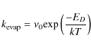
|
(9) |
For those species that are not mobile on the surface default values are
2.4 Reaction set
The basic gas phase reactions are chosen to give a representative model of an interstellar cloud. Beginning with the UMIST astrochemical reaction rates database, RATE95 (Millar et al. 1997), all reactions involving chlorine, phosphorus, iron, silicon, sodium and sulphur are removed along with those involving species with five or more carbon atoms. This yields a reaction set based on hydrogen, helium, carbon, oxygen and nitrogen. Magnesium reactions are included to ensure a token metal and source of electrons. Additional provision is made for species formed only on grain surfaces which can pass into the gas phase. An extra set of reactions allowing gas phase destruction of these species has been added to the gas phase reaction set, listed in the Appendix (Table 19).
The surface phase reaction set (Table 18) is constructed with reference to those reactions provided by Hasegawa et al. (1992) and Hasegawa & Herbst (1993). However it is very much optimized to allow the production of *CH3OH, *C2H5OH and *CH3OCH3. The reactions listed by Hasegawa et al. contain a number of laboratory measured potential energy barriers which slow down the rate of formation of particular species. Only a few such barriers are used here. Further, the reaction set includes almost entirely reactions orientated to the formation of complex molecules. More reactions to produce other species would reduce the complex molecule abundance by draining raw material. It is recognized that this orientation of the reaction set is a limitation of the Gas/Surface model. However, it is regarded as a valid test of the hypothesis of complex molecule formation on grain surfaces. If, given all these advantages, such molecules still could not be produced by grain surface catalysis then the original supposition of such a production method would have to come under deeper scrutiny.
A small number of surface reactions are included that are not
directly involved in complex molecule formation.
These are included because they are are believed to be significant to
overall surface chemistry.
The most basic of all is the grain formation of H2,
whose equation is:
| (10) |
It is considered that the H2 molecule produced passes directly into the gas phase without the need for any specific desorption process. This is consistent with quantum calculations which indicate the resultant molecule is formed with sufficient energy to eject it directly from the surface. Other reactions form small molecules which are frequently seen in high abundances in regions where grain mantles are thought to have recently evaporated. The basis of nitrogen chemistry is formation of *NH3 by the route:
| (11) |
Direct combination of atoms can also form *CN, *NO, *HNO, *HCN and *HNC. *O2 and *OH can also form directly and *OH can further react to form *H2O. Other combination reactions allow the formation of *CO and *CH4. *CO and *H can also react to form *HCO and *H2:
| (12) |
*H2CO can be formed and destroyed by the reactions :
| (13) |
| (14) |
There are two possible routes to *CO2, which is stable on the grain surface and does not react further:
Direct combination of *CO with *O has been omitted as it is believed that this reaction is extremely inefficient (Grim & d'Hendecourt 1986; Breukers 1991). Direct combination of carbon atoms to form *C2 has also been omitted to simplify the surface chemistry. If it occurred it would lead by hydrogenation to the presence of significant amounts of *C2H6, not currently detected. C2H6 is seen in the cometry coma of comets Hyakutake and Hale-Bopp (Mumma et al. 1996) and it is not known if this formed on the surface or in the gas phase. The bulk of surface reactions comprise routes to the complex molecules *CH3OH, *C2H5OH and *CH3OCH3. *CH3OH is formed by combining *CHn and *OH (n = 0-3):
| (17) |
The resultant is then hydrogenated as necessary to form *CH3OH. Alternative routes are provided by:
| (18) |
| (19) |
*COH can then hydrogenate. Reaction between *CO and *H can also produce *HCO and the ratio of the two reactions is controlled by activation energy barriers. Routes to *C2H5OH and *CH3OCH3 involve forming a spine of C-C-O or C-O-C and then hydrogenating until the molecule saturates. This is accomplished by the reactions:
Activation energy barriers can be included which slow down particular reactions. Some are from laboratory measurements. (See Hasegawa et al. 1992, and references therein.) Those for the production of
2.5 Species set and starting abundances
The species set is derived from the reaction set. (Full listing in the Appendix, Tables 16 and 17.) All species can exist in the gas phase while only neutral species exist on the grain surface. Any ion freezing out is assumed to be neutralized. For ions with no neutral equivalent it is assumed they break up in exactly the same way as by electron neutralization in the gas phase. The starting abundances (Table 3) are from Hasegawa et al. (1992). Originally used by Leung et al. (1984) they are believed to be a reasonably accurate representation of the abundances found in an interstellar cloud, particularly one liable to collapse into a hot core or hot corino. Earlier gas phase only models derived using them are consistent with observations within the known accuracy of the chemistry.
Table 3: Gas/Surface model - starting abundances.
3 Model parameters
3.1 Calculating parameters
Table 4: Gas/Surface model - fixed parameters.
As used here only four physical parameters are varied to model
cloud collapse : density, visual extinction, gas temperature and grain
temperature. All other parameters can be regarded as fixed and their
values are given in Table 4.
The definitive factor is density, which controls the speed of collapse.
In all cases here the cloud is assumed to be spherical and of uniform
density.
This is recognized as an approximation,
possible effects of non-uniform density in star forming clouds
are discussed by Shu et al. (1993).
For the cloud to begin to contract under its own self-gravity
its mass must exceed the Jeans mass (MJ)
for its density.
For the cloud densities modelled, the masses and corresponding Jeans
mass are shown in Table 5,
which also gives the relevant free-fall times (
![]() )
and radii.
)
and radii.
Table 5: Gas/Surface model - cloud parameters.
The cloud collapse is halted at a density of 108 cm-3,
observations of hot cores and hot corinos yield densities 10
6-109 cm-3.
As the data in the Appendix demonstrate,
by the end of the collapse all the hydrogen in the cloud has become
molecular.
(H2 abundance = 5.0
![]() with
respect to total hydrogen.)
with
respect to total hydrogen.)
![]() is
calculated from Brown (1988)
and its increase is stopped at 60 mag as further increases in
have negligible effect on the chemistry.
is
calculated from Brown (1988)
and its increase is stopped at 60 mag as further increases in
have negligible effect on the chemistry.
All cloud collapse models presented here assume that gas and
grain temperature are the same.
Since the gas and grains are closely coupled and the temperature mainly
varies as a smooth function it is unlikely
that they would be significantly different over the temperature region
where
the grains have mantles.
As a cloud collapses gravitational energy liberated can be efficiently
radiated in the infrared and submillimeter
bands (Dyson & Williams 1980).
However, at some point the temperature must rise
to begin nuclear processing. It is assumed that below a density of 106 cm-3the
cloud can efficiently radiate and temperature (T)
in this region is found from a curve fitting technique derived by
Tarafdar et al. (1985)
:
where n is number density and

From Tarafdar et al.
Recently a number of hot corinos (Ceccarelli et al. 2004;
Bottinelli et al. 2004)
have been investigated.
These are regions of low mass (![]() 1
1 ![]() )
star formation
embedded within and condensed from molecular clouds. They have typical
sizes of
)
star formation
embedded within and condensed from molecular clouds. They have typical
sizes of ![]() 200 AU,
temperatures of
200 AU,
temperatures of ![]() 100 K
and densities of
100 K
and densities of ![]() 107 cm-3.
(Cazaux et al. 2003;
Bottinelli et al. 2004,
and references within). Complex molecules have been detected in four
hot corino sources, listed in Table 1.
107 cm-3.
(Cazaux et al. 2003;
Bottinelli et al. 2004,
and references within). Complex molecules have been detected in four
hot corino sources, listed in Table 1.
3.2 Collapse scenarios
Table 6: Collapse scenario model parameters.
Table 7: Observed interstellar ices (See text for references).
Table 8: Mantle composition w.r.t H2O at maximum mantle thickness for each model.
In all, eight different cloud collapse scenarios are investigated, designated models 1-8. Models 1-3 are free-fall collapses with starting abundances of 100, 1000 and 10 000 cm-3, regarded as slow, medium and fast. The observed formation rate of new stars is too low for all stars in the galaxy to be formed by free-fall collapse. It is widely asserted that some mechanism supports clouds against collapse, the most commonly suggested being magnetic fields (Shu et al. 1993). For this reason models 4-6 are retarded collapses, again with starting abundances of 100, 1000 and 10 000 cm-3. No specific retardation mechanism is incorporated in the Gas/Surface model nor is one necessary. Retardation is accounted for by arbitrarily slowing down the decrease in radius by a factor of 5.0. This ensures that the cloud takes longer to collapse with corresponding further evolution in the chemistry. Apart from retardation the parameter change in density, gas and grain temperature and visual extinction follows exactly the same pattern as in models 1-3.For the purposes of direct comparison as many parameters as possible are kept constant for all collapses. At a density of 100 cm-3 the hydrogen is likely to be almost completely atomic. Observed clouds of this density are optically thin and exposure to background starlight ensures an ample supply of UV photons to break up H2. At 1000 cm-3 this is still approximately true though some H2 does form. However at the high density case of 10 000 cm-3 it is unphysical. The clouds are sufficiently dense that they will be predominantly H2. For this reason the final models, 7 and 8, replicate the free-fall and retarded collapses from 10 000 cm-3 with their initial hydrogen abundance molecular instead of atomic.
Essensially the chemistry during cloud collapse can be divided into three approximate segments:
- 1.
- Pre-freeze out. Gas phase chemistry dominates, similar to that in gas phase only models.
- 2.
- Freeze out. As the temperature falls and the visual
extinction (
 )
increases (curtailing photodesorption), freeze out occurs and surface
reactions dominate the chemistry. This occurs around the minimum
temperature,
)
increases (curtailing photodesorption), freeze out occurs and surface
reactions dominate the chemistry. This occurs around the minimum
temperature,  10.0
and 10.2 K.
10.0
and 10.2 K.
- 3.
- Post-freeze out. Once the temperature rises the entire grain mantle passes back into the gas phase. Grain surface products are suddenly released into a very dense, warm, dark cloud environment. This leads to a rapidly changing chemistry where a wide variety of different species interact.
4 Discussion
The Appendix contains output data from each of the eight models.
The most abundant gas phase species at both the
plateau point and ![]() years
later
are listed in Tables 19-27.
Variation in gas phase species abundance over time is shown in
Figs. 1-8.
The results are discussed in this section.
years
later
are listed in Tables 19-27.
Variation in gas phase species abundance over time is shown in
Figs. 1-8.
The results are discussed in this section.
4.1 Mantle composition
Table 9: Mantle layering.
Table 10: Gas phase abundances - freeze out.
The test of any theoretical model is to compare it to
observations. Table 7
presents observational data on interstellar ices towards a number of
sources. The abundances shown are relative
to *H2O and have been measured by Boogert
et al. (2008)
for *HCOOH & *CH3OH, Pontoppidan
et al. (2008)
for CO & CO2,
![]() berg
et al. (2008)
for CH4 and Gibb et al. (2000) for *NH3
& *H2CO.
For data taken from Boogert et al. (2008)
measured values have been taken, observations where a lower limit only
has been established have been ommitted. Further Boogert
et al. (2008)
data for *NH+4has been
ommitted as the authors themselves point out that the inclusion of
certain components in the abundance estimation is still a matter of
debate.
berg
et al. (2008)
for CH4 and Gibb et al. (2000) for *NH3
& *H2CO.
For data taken from Boogert et al. (2008)
measured values have been taken, observations where a lower limit only
has been established have been ommitted. Further Boogert
et al. (2008)
data for *NH+4has been
ommitted as the authors themselves point out that the inclusion of
certain components in the abundance estimation is still a matter of
debate.
It is assumed that ice measurements reflect the composition
of grain mantles along the measured lines of sight.
No measurements are available for mantles in hot cores or hot corinos
as within these regions the temperature is sufficiently high
that any grains have been fully thermally desorbed.
Observations made of other, cooler regions are therefore
the best available indicator of grain mantle composition.
All models produce mantles with a predominance of *H2O,
(absolute composition 40-64%), agreeing with observations.
Table ![]() presents mantle composition at greatest thickness as a percentage of *H2O
abundance for all mantle species with abundance
presents mantle composition at greatest thickness as a percentage of *H2O
abundance for all mantle species with abundance ![]() 1% *H2O and for the
complex molecules regardless of their contribution.
Table 9
shows the conditions during each model
when the mantle is at its greatest thickness.
The point of greatest thickness is defined as that timestep with the
largest number of surface layers. Where this is the same for two or
more timesteps the latest is taken.
1% *H2O and for the
complex molecules regardless of their contribution.
Table 9
shows the conditions during each model
when the mantle is at its greatest thickness.
The point of greatest thickness is defined as that timestep with the
largest number of surface layers. Where this is the same for two or
more timesteps the latest is taken.
*CO is well modelled in models 1-4 and 6 and overproduced in the other three. For models 7 and 8 this is a consequence of the molecular hydrogen starting abundance. In both cases atomic carbon and oxygen are able to preferentially combine with each other due to the absence of atomic hydrogen which would otherwise convert them to *H2O and *CH4. Model 5 appears to be an optimum case (with initial atomic hydrogen) for the production of *CO and also subsequently *C2H5OH and *CH3OCH3, hence the higher proportion of all three of these species. Table 10 bears this out, showing an order of magnitude lower carbon abundance at freeze out time in model 5 compared to the other models. Correspondingly both *CO and *CO2 are significantly more abundant in model 5. Both these are preferentially formed in the gas phase before freeze out. *CO2 is well modelled in models 4, 5, 7 and 8 and underproduced in all others. Again in models 7 and 8 the absence of initial atomic hydrogen is the major factor here, while in models 4 and 5 it seems that the longer time period before freeze out enhances *CO2 production, for the same reasons as it also enhances *CO production. Exactly the same factors result in *CH4 being well modelled in models 5, 7 and 8 and overproduced in all others. The faster collapses (models 1, 2, 3 and 6) freeze out atomic carbon before it can form molecules in the gas phase and once on the grain this rapidly hydrogenates into *CH4. Model 4 then appears as a transitory case. It has more *CH4 than model 5, about the same as the faster cases, with correspondingly more *CO and *CO2 than the faster cases and less than model 5. It appears that for model 4 the greater time before freeze out for CO and CO2 to form is partially offset by the lower starting density. The same effect can be seen when comparing models 1 and 2, though it is not as pronounced.
*NH3 is well modelled in
models 1, 2 and 3, above the 1% threshold in model 7
and underproduced in the other models. Here it seems that rapid
collapse alone is the major factor. Abundance in model 7 is
significantly lower than in models 1-3, entirely a consequence
of the molecular hydrogen starting abundance.
Models 4-8 all predict ![]() 1% *HNO.
Correspondingly these are the models with the least *NH3.
The highest *HNO abundance is in models 7 and 8,
again a consequence of the molecular hydrogen starting abundance.
Nitrogen cannot easily form NH3 in the gas or
surface phase due to the lack of atomic hydrogen.
Instead, atomic nitrogen freezes out and combines with *OH to form
*HNO. The lack of atomic hydrogen allows there to be proportionately
more *OH available, which otherwise would hydrogenate to form *H2O.
Models 4 and 5 seem to be intermediate cases, their longer
collapse times
allowing some but not all of the initial gas phase atomic hydrogen to
convert to molecular before freeze out.
1% *HNO.
Correspondingly these are the models with the least *NH3.
The highest *HNO abundance is in models 7 and 8,
again a consequence of the molecular hydrogen starting abundance.
Nitrogen cannot easily form NH3 in the gas or
surface phase due to the lack of atomic hydrogen.
Instead, atomic nitrogen freezes out and combines with *OH to form
*HNO. The lack of atomic hydrogen allows there to be proportionately
more *OH available, which otherwise would hydrogenate to form *H2O.
Models 4 and 5 seem to be intermediate cases, their longer
collapse times
allowing some but not all of the initial gas phase atomic hydrogen to
convert to molecular before freeze out.
*HNO is not currently observed in grain mantles and
is another model prediction to be searched for. However its greatest
abundance occurs in two collapses (models 7 and 8), both with high
starting density.
A dense cloud with ample molecular hydrogen could have evolved
chemically before collapse begins
reducing the *HNO abundance by enabling atomic nitrogen
to combine into other species in the early gas phase.
All models predict a significant mantle abundance of *N2
and most models *O2, at ![]() 10%.
In the absence of observational measurements these must be regarded as
model predictions. Ehrenfreund & van Dishoeck (1998) suggest
possible
ways of searching for *N2 and *O2while
Ehrenfreund & Schutte (2000)
describe the current state of observations.
10%.
In the absence of observational measurements these must be regarded as
model predictions. Ehrenfreund & van Dishoeck (1998) suggest
possible
ways of searching for *N2 and *O2while
Ehrenfreund & Schutte (2000)
describe the current state of observations.
Although mantle composition observations cannot be regarded as complete and definitive, approximate agreement for *H2O and *CO is seen in mantles produced by the Gas/Surface model. Mantle compositions in models 3 and 6 (10 000 cm-3 free fall and retarded) must be regarded as suspect as it is likely that the scenarios themselves are unphysical, starting as they do from atomic hydrogen. Models 4, 5, 7 and 8 produce compositions closest to observations, although models 7 and 8 predict *CH3OH abundance at the low end of its observed abundance range. The effects of collapse timescale on mantle composition are shown in Table 10 which lists relative abundances of gas phase C, CO, CO2, H, H2 and O with respect to total hydrogen at the beginning of freeze out. This is arbitrarily defined, for the purposes of this discussion, as the last timestep before at least five mantle layers form on the grain. Models 2, 4 and particularly 5 seem to have an optimum combination of collapse speed and density to allow significant CO to form in the gas phase. This partially depletes atomic carbon and enables freeze out to occur while there is still some atomic hydrogen available with corresponding consequences for the chemistry thereafter.
4.2 Complex molecules
Table 11: Complex molecule abundances - gas phase.
4.2.1 Complex molecules - surface phase
The prime function of the Gas/Surface model is to investigate the
formation of complex molecules by grain surface catalysis. Gas phase
abundances in the final stages of collapse are governed by surface
abundances prior to mantle desorption.
The mantle abundances with respect to *H2O of *CH3OH,
*C2H5OH and *CH3OCH3
at the greatest mantle thickness for each model are listed in
Table ![]() .
Models 1-6 all produce *CH3OH in the
5-15% range,
agreeing well with observations. Models 7 and 8
produce
.
Models 1-6 all produce *CH3OH in the
5-15% range,
agreeing well with observations. Models 7 and 8
produce ![]() 1%.
This is a consequence of the initial hydrogen being molecular.
*CH3OH requires atomic hydrogen for its
formation
(Sect. 2.4)
and with little available formation is significantly reduced.
1%.
This is a consequence of the initial hydrogen being molecular.
*CH3OH requires atomic hydrogen for its
formation
(Sect. 2.4)
and with little available formation is significantly reduced.
Models 1-6 all produce about the same amount of *C2H5OH
(![]() 0.001%)
while models 7 and 8 produce significantly more (
0.001%)
while models 7 and 8 produce significantly more (![]() 0.025%).
For *CH3OCH3
models 1-4 and 6 produce
0.025%).
For *CH3OCH3
models 1-4 and 6 produce ![]() 0.0000002%
while models 5, 7 and 8 production is higher at
0.0000002%
while models 5, 7 and 8 production is higher at ![]() 0.0001%.
Formation of complex molecules
requires atomic carbon and *CO on the grain, the *CO originating in the
gas phase (Sect. 2.4).
Maximum production takes place when the prior
gas phase has produced significant CO, while leaving sufficient
atomic carbon to form C-C-O and C-O-C structures on the surface after
freeze out. At the same time if there is considerable atomic hydrogen
present at freeze out then this will rapidly hydrogenate atomic carbon
on the grain surface leaving little available to form complex
molecules.
This is demonstrated by models 7 and 8 where the initial
hydrogen is entirely molecular. Absence of much atomic hydrogen leaves
CO to form preferentially in the gas phase. It then freezes out
alongside atomic carbon which cannot readily hydrogenate into *CH4
and so is available to form C-C-O and C-O-C.
Models 7 and 8 show low *CH4,
enhanced *CO and the largest proportions
of both *C2H5OH and *CH3OCH3.
0.0001%.
Formation of complex molecules
requires atomic carbon and *CO on the grain, the *CO originating in the
gas phase (Sect. 2.4).
Maximum production takes place when the prior
gas phase has produced significant CO, while leaving sufficient
atomic carbon to form C-C-O and C-O-C structures on the surface after
freeze out. At the same time if there is considerable atomic hydrogen
present at freeze out then this will rapidly hydrogenate atomic carbon
on the grain surface leaving little available to form complex
molecules.
This is demonstrated by models 7 and 8 where the initial
hydrogen is entirely molecular. Absence of much atomic hydrogen leaves
CO to form preferentially in the gas phase. It then freezes out
alongside atomic carbon which cannot readily hydrogenate into *CH4
and so is available to form C-C-O and C-O-C.
Models 7 and 8 show low *CH4,
enhanced *CO and the largest proportions
of both *C2H5OH and *CH3OCH3.
Table 12: Molecular abundance in a sample of four low-mass protostars (Bottinelli et al. 2007).
Models 1, 2, 3 and 6 with their faster collapse times and initial atomic hydrogen all have significantly lower *CO in the mantle and hence much lower complex molecule abundance. Models 4 and 5 have the longest collapse time of any of the models. This leads to significantly more *CO, in the case of model 5 approximately the same as in the molecular hydrogen starting abundance cases. Model 4 again appears as a transitory case. It has 15% *CO, formed in the gas phase and then frozen out. However its initial low density means that significant atomic hydrogen is present at freeze out and this can hydrogenate the remaining atomic carbon to *CH4 (28%) leaving very little for the production of complex molecules. Model 5 avoids this situation. Here substantial *CO is frozen out but very little atomic hydrogen remains, hence the paucity of *CH4. Much of the remaining carbon has contributed to the high *CO2 abundance (also seen in models 7 and 8) however some has led to the significantly increased *CH3OCH3.
Each model produces a higher mantle abundance for
*C2H5OH than *CH3OCH3.
For models 1-4 and 6 the difference is greater than
3 orders of magnitude
while for models 7 and 8 it is 2 and for model 5 only
1.
The abundance difference seems to be caused by reaction channel
differences.
*C2H5OH forms mainly by
hydrogenation on the grain of C-C-O.
However *CH3OCH3 seems to
form mainly by freeze out from the gas phase.
Its gas phase origin is a two stage process with C2H6OH+
(protonated dimethyl ether) as an intermediate:
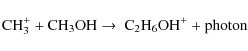
Gas phase C2H6OH+ can also be destroyed by:
Essentially C2H6OH+ is made from CH3OH. Once formed it is then destroyed in forming CH3OCH3(Eq. (25)) which can freeze out onto the grain surface where it is stable or it can form CH3OH (Eq. (26) which is then available to form more C2H6OH+ via Eq. (24). As long as the temperature is low enough to ensure that there is a net freeze out of molecules onto the grain surface this process results in a build up of *CH3OCH3. While workable this gas phase production of CH3OCH3which then freezes out is less efficient than the direct grain surface hydrogenation which produces *C2H5OH in significantly greater abundances. Although production of C2H6OH+ takes place in the gas phase grain surface catalysis is crucial to the process. At the time of freeze out most CH3OH is being produced by evaporation from the grain mantle. In turn the dominant production of *CH3OH is by a chain of direct hydrogenation reactions of *CO.
Comparison of reaction rates of complex molecule formation for the different models shows that model 5 seems to have an optimum combination of parameters to form *CH3OCH3, hence its significantly higher abundance in this model. Table 1 does not show any consistency in C2H5OH : CH3OCH3 ratio and it seems from the models here that the abundance ratio of these two is significantly sensitive to prevailing conditions.
4.2.2 Complex molecules - gas phase
Other than *CH3OH no observations are currently
available of complex molecules in grain mantles. However measurements
do exist of gas phase abundances (Table 12)
and these can be compared to the results of the models
shown in Table 11.
Comparisons are made at the plateau point
and at ![]() years
later,
the end point of time segment 2. Between these two points the model
most closely resembles a hot corino.
There are uncertainties in observations and even when these can be
minimized apparently similar sources yield significantly different
abundance values for the same species. There are further uncertainties
in the chemistry both in the processes of surface chemistry and the
accuracy of gas phase rate coefficients. For these reasons a
model-predicted gas phase abundance
is considered to be in
reasonable agreement with observations if it falls within half an order
of magnitude of the range of observed values
at any time between the plateau point and
years
later,
the end point of time segment 2. Between these two points the model
most closely resembles a hot corino.
There are uncertainties in observations and even when these can be
minimized apparently similar sources yield significantly different
abundance values for the same species. There are further uncertainties
in the chemistry both in the processes of surface chemistry and the
accuracy of gas phase rate coefficients. For these reasons a
model-predicted gas phase abundance
is considered to be in
reasonable agreement with observations if it falls within half an order
of magnitude of the range of observed values
at any time between the plateau point and
![]() years
later.
The acceptable ranges for complex molecules are given in Table 13,
(derived from Table 12).
years
later.
The acceptable ranges for complex molecules are given in Table 13,
(derived from Table 12).
Table 13: Acceptable gas phase fractional abundance ranges for complex molecules.
Table 14: Acceptable gas phase abundance ranges for other molecules.
CH3OH is well modelled in all
scenarios, though the abundance
varies significantly.
In all of models 1-6 (all models starting with atomic
hydrogen)
CH3OH is overproduced at the plateau point and
then for five of these cases falls to within the acceptable range by
![]() years
later.
The sole exception here is model 5 (retarded collapses from
1000 cm-3) where the abundance actually
drops to below the valid range
years
later.
The sole exception here is model 5 (retarded collapses from
1000 cm-3) where the abundance actually
drops to below the valid range
![]() years
later. Since the abundance has passed through the valid range
during the time period
in question this is held to indicate validity. Models 7
& 8 (with molecular hydrogen starting abundance)
are both within the valid range at the plateau point and fall below it
by
years
later. Since the abundance has passed through the valid range
during the time period
in question this is held to indicate validity. Models 7
& 8 (with molecular hydrogen starting abundance)
are both within the valid range at the plateau point and fall below it
by ![]() years
later. In all cases the CH3OH gas phase
abundance declines after the grain mantles are evaporated.
years
later. In all cases the CH3OH gas phase
abundance declines after the grain mantles are evaporated.
CH3OCH3 can also
be considered well modelled in all cases, though its behaviour is more
diverse.
Models 1, 2 and 3 are within acceptable range at the plateau point and
by ![]() years
later
abundance has actually increased, suggesting further production in the
gas phase.
At this time model 2 is still within the acceptable range while 1
& 3 overproduce.
Models 4, 5, and 6 all overproduce slightly at the plateau point while
years
later
abundance has actually increased, suggesting further production in the
gas phase.
At this time model 2 is still within the acceptable range while 1
& 3 overproduce.
Models 4, 5, and 6 all overproduce slightly at the plateau point while
![]() years
later
abundances have dropped to within acceptable range for models 4
& 6 and below acceptable range for model 5.
As with CH3OH model 5 CH3OCH3
abundance is considered to be validly modelled as it has passed through
the acceptable range during the relevant time period. In this case the
preciptious drop, 4 orders of magnitude, serves to illustrate how
volatile the chemistry becomes in the period after the grain mantles
evaporate. Models 7 and 8 show a similar behaviour being within
acceptable range at the
plateau point and also dropping by 4 orders of magnitude 2.0
years
later
abundances have dropped to within acceptable range for models 4
& 6 and below acceptable range for model 5.
As with CH3OH model 5 CH3OCH3
abundance is considered to be validly modelled as it has passed through
the acceptable range during the relevant time period. In this case the
preciptious drop, 4 orders of magnitude, serves to illustrate how
volatile the chemistry becomes in the period after the grain mantles
evaporate. Models 7 and 8 show a similar behaviour being within
acceptable range at the
plateau point and also dropping by 4 orders of magnitude 2.0 ![]() 105 years later.
105 years later.
Table 15: Other molecule abundances - gas phase.
Table 16: Gas/Surface model - surface phase species set.
Table 18: Solid phase reactions used for complex molecule formation.
As discussed in Sects. 4.1 and 4.2.1 the production of complex molecules is dependent on the gas phase abundances of atomic carbon and hydrogen at the point of freeze out. Gas phase processes are considerably better understood than surface processes, and in particular the potential barriers used could be different leading to changes in the relative proportions of species. With these caveats we conclude that complex molecules, seen in both hot cores and hot corinos, can be made in the observed abundances by grain surface catalysis processes. Ethanol (C2H5OH) production has been included in the models here as it is frequently seen in the same environments as dimethyl ether (CH3OCH3) (Table 1). Currently it has not been observed in hot corinos and the abundances modelled here must be regarded as predictions awaiting the test of observation. The only major distinction that can be draw between the different models is between those starting with molecular hydrogen (models 7 & 8) compared to the other six. As would be expected the lack of initial atomic hydrogen stifles the production of those molecular species which require it. Correspondingly this then allows higher abundances of other species whose raw material would otherwise have been removed by combination with atomic hydrogen. No correlation is noticable in the production of complex molecules in either gas or surface phase with the cloud starting mass and/or collapse time. This may be indicative of a volatile chemistry and/or of the limitations of our current understanding.
Table 12 lists observational measurements for a number of other molecules observed in hot corinos. These too can be compared to the models here as a validity check. HCOOH and C2H5CN are not in the Gas/Surface model reaction set as used here.
Both of these two species are obvious candidates for inclusion
in future modelling.
HCOOH may be particularly significant as both gas (Table 12)
and solid phase (Table 7)
data are now available for it.
Both Bottinelli et al. (2007) and
Fuente et al. (2005)
point out that HCOOH shows significantly different abundance behaviour
between
corino type objects, as modelled here, and higher temperature hot
cores,
unlike a majority of other observed species. The reasons for this are
not known
but present an interesting issue for prospective future models.
H2CO, HCOOCH3 and CH3CN
are included and their abundances are listed in Table 15.
The same criteria for acceptable range is used as above, namely a gas
phase abundance is considered to be in reasonable agreement with
observations if it falls within half an order of magnitude of the range
of observed values
at any time between the plateau point and
![]() years
later.
Relevant values are shown in Table 14.
years
later.
Relevant values are shown in Table 14.
H2CO is well modelled in all collapse
scenarios. Table 12
lists only abundance data for HCOOCH3-A.
Bottinelli et al. (2007),
from where this data is taken,
state that the abundance of the E form of HCOOCH3is
usually very close to that of the A form
and that they regard the HCOOCH3 total abundance
to be twice that of HCOOCH3-A.
For this reason the acceptable range of HCOOCH3
is given in Table 14
as ![]() -
-
![]() ,
i.e., half an order of magnitude above and below double the HCOOCH3-A
abundance. Modelled HCOOCH3 is underabundant at
the plateau point in all cases. By
,
i.e., half an order of magnitude above and below double the HCOOCH3-A
abundance. Modelled HCOOCH3 is underabundant at
the plateau point in all cases. By
![]() years
later it remains underabundant in seven of the eight cases. Only in
model 2 does it rise above the acceptable lower limit. CH3CN
is well modelled in most of the cases.
In models 1-4 & 6 it is within the acceptable range
both at the plateau point
and
years
later it remains underabundant in seven of the eight cases. Only in
model 2 does it rise above the acceptable lower limit. CH3CN
is well modelled in most of the cases.
In models 1-4 & 6 it is within the acceptable range
both at the plateau point
and ![]() years
later. In models 5 & 8 it is always underabundant. In model 7
it is within acceptable range at the plateau point and has fallen to
below it by
years
later. In models 5 & 8 it is always underabundant. In model 7
it is within acceptable range at the plateau point and has fallen to
below it by ![]() years later. For all three of these molecules there is no descernible
correlation between abundance produced and cloud starting mass and/or
collapse time.
years later. For all three of these molecules there is no descernible
correlation between abundance produced and cloud starting mass and/or
collapse time.
5 Conclusion
Overall the Gas/Surface model as used here reproduces to a reasonable degree the observed complex molecule abundances seen in hot corinos. In particular abundance values produced for methanol and dimethyl ether are comparable to those observed in both gas and surface phases.
The surface phase molecular abundances produced by the model reflect the starting conditions, particularly the nature of the initial hydrogen - atomic or molecular. This determines the degree of processing in the initial gas phase and hence the abundance of species frozen on to the dust and available for surface chemistry. This in turn allows an understanding of the differences in grain mantle composition observed in different regions. The model results clearly indicate that both the starting conditions and particularly the timescale of collapse are major contributors to the overall chemistry.
A number of other workers in the area have reached similar conclusions. Garrod & Herbst (2006) specifically investigated methyl formate (HCOOCH3). They concluded that its formation required the grain surface production of precursor molecules which were then released into the gas phase to produce methyl formate itself. This tallies with the similar behaviour seen here although Garrod & Herbst were able to produce abundances closer to observed values. They suggest a similar pattern for dimethyl ether, exactly as the Gas/Surface model shows. Later applications of the same model produced comparable results. Aikawa et al. (2008) consider a collapse case where again large organic species (or their immediate precursors) are formed on grain mantles before evaporation into the gas phase. Observed abundances can be both well modelled or over and under produced depending on starting conditions and timescale. Garrod et al. (2008) apply their model to more general star formation cases and note specifically that the longer the time available for grain surface chemistry to progress the more complex the eventual gas phase chemistry becomes. In this case agreement with observations is seen for abundances of ethanol and dimethyl ether though not for some other complex molecules. Hassel et al. (2008) specifically model L1529, a lukewarm corino, which may be the prototype of a new class of such objects. Their analysis demonstrates that, at least in the case of L1529, there is some difficulty in establishing definitvely how a particular chemical state came to evolve and a number of scenarios are possible depending on the length of time the corino spent in each particular phase.
In conclusion then grain surface processing, combined with the variation of physical conditions modelled here, can be regarded as a viable method for the formation of complex molecules, particularly ethanol and dimethyl ether, in the environment found in the vicinity of a hot corino and produce abundances comparable to those actually observed.
AcknowledgementsAstrophysics at Queens University Belfast is supported by a grant from STFC. P. Hall wishes to thank Professor H. Fleischmann of Cornell University Department of Applied and Engineering Physics for helpful conversations about optical absorbtion. We both wish to thank an anonymous referee whose comments improved an earlier version of this paper.
References
- Aikawa, Y., Wakelam, V., Garrod, R. T., & Herbst, E. 2008, ApJ, 674, 984 [NASA ADS] [CrossRef] [Google Scholar]
- Allen, M., & Robinson, G. W. 1977, ApJ, 212, 396 [NASA ADS] [CrossRef] [Google Scholar]
- Ball, J. A. 1970, ApJ, 162, L203 [NASA ADS] [CrossRef] [Google Scholar]
- Boogert, A. C. A., Schutte, W. A., Tielens, A. G. G. M., et al. 1996, A&A, 315, L377 [NASA ADS] [Google Scholar]
- Boogert, A. C. A., Pontoppidan, K. M., Knez, C., et al. 2008, ApJ, 678, 985 [NASA ADS] [CrossRef] [Google Scholar]
- Bottinelli, S., Ceccarelli, C., Lefloch, B., et al. 2004, ApJ, 615, 354 [NASA ADS] [CrossRef] [Google Scholar]
- Bottinelli, S., Ceccarelli, C., Williams, J. P., et al. 2007, A&A, 463, 601 [NASA ADS] [CrossRef] [EDP Sciences] [Google Scholar]
- Breukers, R. J. L. H. 1991, Ph.D. Thesis University of Leiden [Google Scholar]
- Brown, P. D. 1988, Ph.D. Thesis University of Manchester [Google Scholar]
- Carral, P., & Welch, W. J. 1992, ApJ, 385, 244 [NASA ADS] [CrossRef] [Google Scholar]
- Caselli, P., Hasegawa, T. I., & Herbst, E. 1993, ApJ, 408, 548 [NASA ADS] [CrossRef] [Google Scholar]
- Cazaux, S., Tielens, A. G. G. M., Ceccarelli, C., et al. 2003, ApJ, 593, L51 [NASA ADS] [CrossRef] [Google Scholar]
- Ceccarelli, C. 2004, in Star Formation in the Interstellar Medium, 195, ed. D. Johnstone, F. C. Adams, F. N. C Lin, D. A. Neufeld, & E. C. Ostriker, ASP Conf. Ser. 323 [Google Scholar]
- Ceccarelli, C., Loinard, L., Castets, A., Tielens, A. G. G. M., & Caux, E. 2000, A&A, 357, L9 [NASA ADS] [Google Scholar]
- Charnley, S. B., Tielens, A. G. G. M., & Millar, T. J. 1992, ApJ, 399, L71 [NASA ADS] [CrossRef] [Google Scholar]
- Charnley, S. B., Kress, M. E., Tielens, A. G. G. M., et al. 1995, ApJ, 448, 232 [NASA ADS] [CrossRef] [Google Scholar]
- De Pree, C. G., Rodriguez, L. F., Dickel, H. R., et al. 1995, ApJ, 447, 220 [NASA ADS] [CrossRef] [Google Scholar]
- Draine, B. T. 1978, ApJS, 36, 595 [NASA ADS] [CrossRef] [Google Scholar]
- Duley, W. W., & Williams, D. A. 1984, Interstellar Chemistry (Academic Press) [Google Scholar]
- Dyson, J. E., & Williams, D. A. 1980, Physics of the Interstellar Medium, (Manchester University Press) [Google Scholar]
- Ehrenfreund, P., & van Dishoeck, E. F. 1998, Adv. Space Res., 21, 15 [Google Scholar]
- Ehrenfreund, P., & Schutte, W. A. 2000, Advances in Space Research, 25, 2177 [Google Scholar]
- Fuente, A., Neri, R., & Caselli, P. 2005, A&A, 444, 481 [NASA ADS] [CrossRef] [EDP Sciences] [Google Scholar]
- Garrod, R. T., & Herbst, E. 2006, A&A, 457, 927 [NASA ADS] [CrossRef] [EDP Sciences] [Google Scholar]
- Garrod, R. T., Wakelam, V., & Herbst, E. 2007, A&A, 467, 1103 [NASA ADS] [CrossRef] [EDP Sciences] [Google Scholar]
- Garrod, R. T., Widicus Weaver, S. L., & Herbst, E. 2008, ApJ, 682, 283 [NASA ADS] [CrossRef] [Google Scholar]
- Garrod, R. T., Vasyunin, A. I., Semenov, D. A., Wiebe, D. S., Henning, Th. 2009, ApJ, 700, L43 [Google Scholar]
- Gibb, E. L., Whittet, D. C. B., Schutte, W. A., et al. 2000, ApJ, 536, 347 [NASA ADS] [CrossRef] [Google Scholar]
- Grim, R. J. A., & d'Hendecourt, L. B. 1986, A&A, 167, 161 [NASA ADS] [Google Scholar]
- Hall, P. 1997, in Dust and Molecules in Evolved Stars, 203, ed. I. Cherchneff, & T. J. Millar (Kluwer Academic Publishers) [Google Scholar]
- Hasegawa, T. I., & Herbst, E. 1993, MNRAS, 261, 83 [NASA ADS] [CrossRef] [Google Scholar]
- Hasegawa, T. I., Herbst, E. & Leung, C. M. 1992, ApJS, 82, 167 [NASA ADS] [CrossRef] [Google Scholar]
- Hassel, G. E., Herbst, E., & Garrod, R. T. 2008, ApJ, 681, 1385 [NASA ADS] [CrossRef] [Google Scholar]
- Herbst, E., & Leung, C. M. 1989, ApJS, 69, 271 [NASA ADS] [CrossRef] [EDP Sciences] [Google Scholar]
- Hindmarsh, A. C. 1974, Lawrence Livermore Laboratory Rept. ucrl-30001 Rev.3 [Google Scholar]
- Hindmarsh, A. C. 1983, In Scientific Computing, 55, ed. R. S. Stepleman, et al. North-Holland Amsterdam [Google Scholar]
- Hollenbach, D. J., & Salpeter, E. E. 1971, ApJ, 163, 155 [NASA ADS] [CrossRef] [Google Scholar]
- Ikeda, M., Ohishi, M., Nummelin, A., et al. 2001, ApJ, 560, 792 [NASA ADS] [CrossRef] [Google Scholar]
- Ikeda, M., Ohishi, M., Nummelin, A., et al. 2002, ApJ, 571, 560 [NASA ADS] [CrossRef] [Google Scholar]
- Jørgensen, J. K., Bourke, T. L., Myers, P. C., et al. 2005, ApJ, 632, 973 [NASA ADS] [CrossRef] [Google Scholar]
- Lacy, J. H., Faraji, H., Sandford, S. A., et al. 1998, ApJ, 501, L105 [NASA ADS] [CrossRef] [PubMed] [Google Scholar]
- Leung, C. M., Herbst, E., & Huebner, W. F. 1984, ApJS, 56, 231 [NASA ADS] [CrossRef] [Google Scholar]
- Maret, S., Ceccarelli, C., Caux, E., et al. 2004, A&A, 416, 577 [NASA ADS] [CrossRef] [EDP Sciences] [Google Scholar]
- Maret, S., Ceccarelli, C., Tielens, A. G. G. M., et al. 2005, A&A, 442, 527 [NASA ADS] [CrossRef] [EDP Sciences] [Google Scholar]
- Millar, T. J. 1990, in Molecular Astrophysics, 115, ed. T. W. Hartquist (University of Cambridge Press) [Google Scholar]
- Millar, T. J., Bennett, A., Rawlings, J. M. C., et al. 1991, A&AS, 87, 585 [NASA ADS] [Google Scholar]
- Millar, T. J., Herbst, E., & Charnley, S. B. 1991, ApJ, 369, 147 [NASA ADS] [CrossRef] [Google Scholar]
- Millar, T. J., Farquhar, P. R. A., & Willacy, K. 1997, A&AS, 121, 139 [NASA ADS] [CrossRef] [EDP Sciences] [Google Scholar]
- Mumma, M. J., Disanti, M. A., dello Russo, N., et al. 1996, Science, 272, 1310 [NASA ADS] [CrossRef] [PubMed] [Google Scholar]
- Öberg, K. I., Boogert, A. C. A., Pontoppidan, K. M., et al. 2008, ApJ, 678, 1032 [NASA ADS] [CrossRef] [Google Scholar]
- Pontoppidan, K. M., Boogert, A. C. A., Fraser, H. J., et al. 2008, ApJ, 678, 1005 [NASA ADS] [CrossRef] [Google Scholar]
- Remijan, A., Snyder, L. E., Friedel, D. N., et al. 2003, ApJ, 590, 314 [NASA ADS] [CrossRef] [Google Scholar]
- Schutte, W. A., & Greenberg, J. M. 1988, in Dust in the Universe, 403, ed. M. E. Bailey, & D. A. Williams (Cambridge University Press) [Google Scholar]
- Shalabiea, O. M. 1995, Ph.D. Thesis University of Leiden [Google Scholar]
- Shalabiea, O. M., & Greenberg, J. M. 1995, A&A, 303, 233 [NASA ADS] [Google Scholar]
- Shu, F., et al. 1993, In Protostars and Planets III, 3, ed. E. H. Levy, & J. I. Lunine (University of Arizona Press) [Google Scholar]
- Snyder, L. E., Buhl, D., Schwartz, P. R., et al. 1974, ApJ, 191, L79 [NASA ADS] [CrossRef] [Google Scholar]
- Spitzer, L. J. 1978, Physical Processes in the Interstellar Medium (Wiley International) [Google Scholar]
- Spitzer, L. J., & Cochran, W. D. 1973, ApJ, 186, L23 [NASA ADS] [CrossRef] [Google Scholar]
- Tapia, M., Persi, P., & Roth, M. 1996, A&A, 316, 102 [NASA ADS] [Google Scholar]
- Tarafdar, S. P., Prasad, S. S., Huntress, W. T., Jr., et al. 1985, ApJ, 289, 220 [NASA ADS] [CrossRef] [Google Scholar]
- Tielens, A. G. G. M., & Hagen, W. 1982, A&A, 114, 245 [NASA ADS] [Google Scholar]
- Tielens, A. G. G. M., & Allamandola, L. J. 1987, In Interstellar Processes, 397, ed. D. J. Hollenbach, & H. A. Thronson (Dordrecht: Kluwer) [Google Scholar]
- Tielens, A. G. G. M., & Charnley, S. B. 1997, Origins of Life and Evoloution of the Biosphere, 27, 34 [Google Scholar]
- van Dishoeck, E. F., & Black, J.C. 1986, ApJS, 62, 109 [NASA ADS] [CrossRef] [Google Scholar]
- Völk, H. J., Jones, F. C., Morfill, G. E., et al. 1980, A&A, 85, 316 [NASA ADS] [Google Scholar]
- Wagenblast, R. 1992, MNRAS, 259, 155 [NASA ADS] [Google Scholar]
- Whittet, D. C. B. 1992, Dust in the Galatic Environment (Institute of Physics Publishing) [Google Scholar]
- Willacy, K. 1993, Ph.D. Thesis University of Manchester [Google Scholar]
- Willacy, K., & Millar, T. J. 1998, MNRAS, 298, 562 [NASA ADS] [CrossRef] [Google Scholar]
- Zuckerman, B., Turner, B. E., Johnson, D. R., et al. 1975, ApJ, 196, L99 [NASA ADS] [CrossRef] [Google Scholar]
Online Material
Table 19: Gas phase reactions used for complex molecule destruction.
Table 20: Model 1 - Free fall collapse from 100 cm-3 - most abundant gas phase species.
Table 21: Model 2 - Free fall collapse from 1000 cm-3 - most abundant gas phase species.
Table 22: Model 3 - Free fall collapse from 10 000 cm-3 - most abundant gas phase species.
Table 23: Model 4 - Retarded collapse from 100 cm-3 - most abundant gas phase species.
Table 24: Model 5 - Retarded collapse from 1000 cm-3 - most abundant gas phase species.
Table 25: Model 6 - Retarded collapse from 10 000 cm-3 - most abundant gas phase species.
Table 26: Model 7 - Free fall collapse from 10 000 cm-3 - H2 starting abundance - most abundant gas phase species.
Table 27: Model 8 - Retarded collapse from 10 000 cm-3 - H2 starting abundance - most abundant gas phase species.
![\begin{figure}
\par\includegraphics[width=15cm,clip]{f1.eps}
\end{figure}](/articles/aa/full_html/2010/09/aa11159-08/img261.png)
|
Figure 1: Model 1 - Free fall collapse from 100 cm-3 - gas phase data. |
| Open with DEXTER | |
![\begin{figure}
\par\includegraphics[width=15cm,clip]{f2.eps}
\end{figure}](/articles/aa/full_html/2010/09/aa11159-08/img262.png)
|
Figure 2: Model 2 - Free fall collapse from 1000 cm-3 - gas phase data. |
| Open with DEXTER | |
![\begin{figure}
\par\includegraphics[width=15cm,clip]{f3.eps}
\end{figure}](/articles/aa/full_html/2010/09/aa11159-08/img263.png)
|
Figure 3: Model 3 - Free fall collapse from 10 000 cm-3 - gas phase data. |
| Open with DEXTER | |
![\begin{figure}
\par\includegraphics[width=15cm,clip]{f4.eps}
\end{figure}](/articles/aa/full_html/2010/09/aa11159-08/img264.png)
|
Figure 4: Model 4 - Retarded collapse from 100 cm-3 - gas phase data. |
| Open with DEXTER | |
![\begin{figure}
\par\includegraphics[width=15cm,clip]{f5.eps}
\end{figure}](/articles/aa/full_html/2010/09/aa11159-08/img265.png)
|
Figure 5: Model 5 - Retarded collapse from 1000 cm-3 - gas phase data. |
| Open with DEXTER | |
![\begin{figure}
\par\includegraphics[width=15cm,clip]{f6.eps}
\end{figure}](/articles/aa/full_html/2010/09/aa11159-08/img266.png)
|
Figure 6: Model 6 - Retarded collapse from 10 000 cm-3 - gas phase data. |
| Open with DEXTER | |
![\begin{figure}
\par\includegraphics[width=15cm,clip]{f7.eps}
\end{figure}](/articles/aa/full_html/2010/09/aa11159-08/img267.png)
|
Figure 7: Model 7 - Free fall collapse from 10 000 cm-3 - H2 starting abundance - gas phase data |
| Open with DEXTER | |
![\begin{figure}
\par\includegraphics[width=15cm,clip]{f8.eps}
\end{figure}](/articles/aa/full_html/2010/09/aa11159-08/img268.png)
|
Figure 8: Model 8 - Retarded collapse from 10 000 cm-3 - H2 starting abundance - gas phase data. |
| Open with DEXTER | |
Footnotes
- ... mantles
- Tables 19-27 and Figures 1-8 are only available in electronic form at http://www.aanda.org
All Tables
Table 1: Observed fractional abundances of complex molecules.
Table 2: Mobile surface species.
Table 3: Gas/Surface model - starting abundances.
Table 4: Gas/Surface model - fixed parameters.
Table 5: Gas/Surface model - cloud parameters.
Table 6: Collapse scenario model parameters.
Table 7: Observed interstellar ices (See text for references).
Table 8: Mantle composition w.r.t H2O at maximum mantle thickness for each model.
Table 9: Mantle layering.
Table 10: Gas phase abundances - freeze out.
Table 11: Complex molecule abundances - gas phase.
Table 12: Molecular abundance in a sample of four low-mass protostars (Bottinelli et al. 2007).
Table 13: Acceptable gas phase fractional abundance ranges for complex molecules.
Table 14: Acceptable gas phase abundance ranges for other molecules.
Table 15: Other molecule abundances - gas phase.
Table 16: Gas/Surface model - surface phase species set.
Table 18: Solid phase reactions used for complex molecule formation.
Table 19: Gas phase reactions used for complex molecule destruction.
Table 20: Model 1 - Free fall collapse from 100 cm-3 - most abundant gas phase species.
Table 21: Model 2 - Free fall collapse from 1000 cm-3 - most abundant gas phase species.
Table 22: Model 3 - Free fall collapse from 10 000 cm-3 - most abundant gas phase species.
Table 23: Model 4 - Retarded collapse from 100 cm-3 - most abundant gas phase species.
Table 24: Model 5 - Retarded collapse from 1000 cm-3 - most abundant gas phase species.
Table 25: Model 6 - Retarded collapse from 10 000 cm-3 - most abundant gas phase species.
Table 26: Model 7 - Free fall collapse from 10 000 cm-3 - H2 starting abundance - most abundant gas phase species.
Table 27: Model 8 - Retarded collapse from 10 000 cm-3 - H2 starting abundance - most abundant gas phase species.
All Figures
|
|
Figure 1: Model 1 - Free fall collapse from 100 cm-3 - gas phase data. |
| Open with DEXTER | |
| In the text | |
|
|
Figure 2: Model 2 - Free fall collapse from 1000 cm-3 - gas phase data. |
| Open with DEXTER | |
| In the text | |
|
|
Figure 3: Model 3 - Free fall collapse from 10 000 cm-3 - gas phase data. |
| Open with DEXTER | |
| In the text | |
|
|
Figure 4: Model 4 - Retarded collapse from 100 cm-3 - gas phase data. |
| Open with DEXTER | |
| In the text | |
|
|
Figure 5: Model 5 - Retarded collapse from 1000 cm-3 - gas phase data. |
| Open with DEXTER | |
| In the text | |
|
|
Figure 6: Model 6 - Retarded collapse from 10 000 cm-3 - gas phase data. |
| Open with DEXTER | |
| In the text | |
|
|
Figure 7: Model 7 - Free fall collapse from 10 000 cm-3 - H2 starting abundance - gas phase data |
| Open with DEXTER | |
| In the text | |
|
|
Figure 8: Model 8 - Retarded collapse from 10 000 cm-3 - H2 starting abundance - gas phase data. |
| Open with DEXTER | |
| In the text | |
Copyright ESO 2010
Current usage metrics show cumulative count of Article Views (full-text article views including HTML views, PDF and ePub downloads, according to the available data) and Abstracts Views on Vision4Press platform.
Data correspond to usage on the plateform after 2015. The current usage metrics is available 48-96 hours after online publication and is updated daily on week days.
Initial download of the metrics may take a while.