| Issue |
A&A
Volume 516, June-July 2010
|
|
|---|---|---|
| Article Number | A72 | |
| Number of page(s) | 12 | |
| Section | Planets and planetary systems | |
| DOI | https://doi.org/10.1051/0004-6361/201014275 | |
| Published online | 02 July 2010 | |
Oort cloud formation at various Galactic distances
R. Brasser1 - A. Higuchi2 - N. Kaib3
1 - Dept. Cassiopée, University of Nice - Sophia Antipolis, CNRS, Observatoire de la Côte d'Azur, Nice, France
2 -
Dept. of Earth and Planetary Science, Tokyo Institute of Technology,
Ookayama, Meguru-ku, Tokyo, Japan
3 -
Astronomy Department, University of Washington, Seattle, WA, USA
Received 17 February 2010 / Accepted 17 March 2010
Abstract
In this study we present the results from numerical simulations of
the formation of the Oort comet cloud where we positioned the Sun in
various parts of the disc of the Galaxy, starting at 2 kpc up to
20 kpc from the Galactic centre. All simulations were run for
4 Gyr. We report that the final trapping efficiency of comets in
the Oort cloud is approximately 4% and is almost independent of the
solar distance from the Galactic centre. This efficiency is not enough
to explain the flux of long-period comets and be consistent with the
mass of the protoplanetary disc. In addition, the population ratio
between the Oort clouds and their corresponding scattered discs is at
least two orders of magnitude lower than observed today. Solar
migration from the inner regions of the Galaxy - where the initial
trapping efficiency is higher - to farther regions - where the
retention is higher - does not add enough of an effect to increase the
efficiency to the necessary value of approximately 20%, so that other
mechanisms for forming the Oort cloud need to be investigated.
Key words: comets: general ; Oort cloud
1 Introduction
Ever since Oort (1950)
published his results on the orbital energy distribution of long-period
and new comets nearly sixty years ago,
astronomers have studied the formation and evolution of this
quasi-spherical cloud of comets surrounding the Sun. Most studies to
date have
concentrated on its formation and evolution in our current Solar System
and with the Sun at its current distance from the Galactic centre on
a circular, coplanar orbit. One such study was performed by Dones
et al. (2004) - based on the model of Levison et al. (2001)
- to
simulate the formation of the Oort cloud in the current Galactic
environment, starting with test particles on nearly circular, nearly
planar
orbits with the giant planets on their current orbits. After 4![]() Gyr their results have shown that only 2.5% of comets ended up in the
outer
cloud (semi-major axis a >20 000 AU; Hills 1981), down from about 5% around 1
Gyr their results have shown that only 2.5% of comets ended up in the
outer
cloud (semi-major axis a >20 000 AU; Hills 1981), down from about 5% around 1![]() Gyr, while the overall efficiency of depositing
material in the cloud after 4
Gyr, while the overall efficiency of depositing
material in the cloud after 4![]() Gyr is about 5% (down from 7.5% at 1
Gyr is about 5% (down from 7.5% at 1![]() Gyr). The inner and outer clouds contain roughly equal mass.
Kaib
& Quinn (2008) have performed similar simulations to those of Dones et al. (2004)
and report only 1% of their comets winding up in the
outer Oort cloud after 4.5 Gyr. These low efficiencies are
difficult to reconcile with the estimated mass in solids in the
primordial
solar nebula and planet migration.
Gyr). The inner and outer clouds contain roughly equal mass.
Kaib
& Quinn (2008) have performed similar simulations to those of Dones et al. (2004)
and report only 1% of their comets winding up in the
outer Oort cloud after 4.5 Gyr. These low efficiencies are
difficult to reconcile with the estimated mass in solids in the
primordial
solar nebula and planet migration.
The problems associated with the above studies were highlighted by the results of Kaib & Quinn (2009), who conclude that most long-period comets (LPCs) could originate in the inner Oort cloud rather than the outer Oort cloud because of a newly-discovered dynamical path connecting the two. In the most extreme case, their results indicate that the outer Oort cloud could be devoid of comets and that all the LPCs originate in the inner cloud. This result requires a new approach to Oort cloud formation and evolution because the aim has shifted from depositing most objects in the outer Oort cloud to building a more substantial inner Oort cloud.
Depositing these comets is a problem in itself. Kaib & Quinn (2009) claim that the Oort cloud contains approximately
![]() kilometre-sized comets, although this number is fairly uncertain because it is based on the observed LPC flux (Francis 2005); the number of
comets in the cloud probably varies between
kilometre-sized comets, although this number is fairly uncertain because it is based on the observed LPC flux (Francis 2005); the number of
comets in the cloud probably varies between
![]() .
Since it is likely that the Oort
cloud formed in two stages (Brasser 2008) and that there were approximately
1012 kilometre-sized bodies available to deposit in the cloud during the second stage (Morbidelli et al. 2009),
the efficiency of
depositing material in the cloud in the current environment of the Sun
is almost an order of magnitude too low if the cloud was generated
solely during the second stage.
.
Since it is likely that the Oort
cloud formed in two stages (Brasser 2008) and that there were approximately
1012 kilometre-sized bodies available to deposit in the cloud during the second stage (Morbidelli et al. 2009),
the efficiency of
depositing material in the cloud in the current environment of the Sun
is almost an order of magnitude too low if the cloud was generated
solely during the second stage.
Star clusters are able to increase the trapping efficiency of comets in the inner Oort cloud during the
first stage (Brasser et al. 2006; Kaib & Quin 2008) but then aerodynamic gas drag prevents kilometre-sized bodies from entering the cloud
(Brasser et al. 2007)
so that in the most extreme case the first stage did not make any
contribution to the cloud. Even if gas drag is not
a problem, the star clusters that are able to produce 90 377 Sedna
have an Oort cloud that is devoid of comets farther than 5000 AU
from
the Sun, and the mechanism of Kaib & Quinn (2009) does not work at shorter distances.
The transfer of comets with a<5000 AU to
orbits with
a>5000 AU is not efficient enough to supply the number of comets of Kaib & Quinn (2009) unless the mass of the disc between 5
and 15 AU during the first stage exceeded 150
![]() (Brasser 2008).
In summary, the dilemma of reconciling the low trapping
efficiency with the flux of LPCs and the existence of Sedna still needs to be solved.
(Brasser 2008).
In summary, the dilemma of reconciling the low trapping
efficiency with the flux of LPCs and the existence of Sedna still needs to be solved.
Here we make an attempt to resolve some of these issues by changing one parameter that has been kept constant in the previously mentioned studies: the strength of the Galactic tides. This is accomplished by varying the location of the Sun in the Galaxy, and thus corresponds to a change in the local density. This variation in distance is justified by evidence that the Sun migrated because of encounters with spiral arms, and it could have been scattered in and out many times yet remained on a nearly circular orbit (Sellwood & Binney 2002). The same study shows that the current orbit of the Sun is consistent with an origin between 4 kpc and 12 kpc from the centre of the Galaxy. In all likelihood the Sun's birthplace cannot be traced because of its chaotic dynamics within the Galactic disc, but perhaps some information can be gained from the Oort cloud. In addition, we can investigate whether the problem of trapping efficiency and LPC flux can be solved if the Sun had resided in different parts of the Galaxy.
One question that demands an answer up front is how this study is different from those in Brasser et al. (2006) and Kaib & Quinn (2008), who studied the formation of the Oort cloud while the Sun was in a star cluster, because the latter studies were able to deposit a much higher percentage of comets in the Oort cloud than the standard model of Dones et al. (2004). The problem with both of these studies was highlighted by Brasser et al. (2007), who showed that aerodynamic gas drag from the solar nebula prevented small comets from reaching the Oort cloud, so that it is possible that all the comets must have arrived later. This second phase of Oort cloud formation happened approximately 600 Myr after the cluster stage during what is called the late heavy bombardment - a global instability in the outer solar system that triggered an intense bombardment of the terrestrial planets (Tsiganis et al. 2005; Gomes et al. 2005) - and if the Sun was in its current Galactic location, we are back to square one. However, if the Sun was in a different part of the Galaxy, preferably closer to the Galactic centre than it is today, then the possibility exists of trapping more comets in the cloud. This scenario is what we aim to investigate here.
The outline for this paper is as follows. In Sect. 2 theoretical considerations are discussed and some predictions are made regarding the inner edge and extent of Oort clouds surrounding solar type stars in other parts of the Galaxy; trapping efficiencies and erosion timescales are also discussed. In Sect. 3 we describe our numerical methods. Section 4 shows the results of the numerical simulations. In Sect. 5 we discuss some of the results, and in the final section conclusions are drawn.
2 Theoretical considerations
The most widely used model for computing the force on a comet caused
by the Galactic tidal field is the one proposed by Heisler &
Tremaine
(1986). In a rotating co-ordinate system where the
![]() -axis points away from the Galactic centre, the
-axis points away from the Galactic centre, the
![]() -axis
is towards the south Galactic pole, and the
-axis
is towards the south Galactic pole, and the
![]() -axis is perpendicular to these according to the right-hand rule (Levison
et al.
2001), the force is given by
-axis is perpendicular to these according to the right-hand rule (Levison
et al.
2001), the force is given by
![\begin{displaymath}\vec{F}_{\rm G} =
(A-B)(3A+B)\tilde{x}\hat{\tilde{x}}-(A-B)^2...
...{y}}-
[4\pi G\rho_{\rm G}-2(B^2-A^2)]\tilde{z}\hat{\tilde{z}},
\end{displaymath}](/articles/aa/full_html/2010/08/aa14275-10/img14.png)
where A and B are the Oort constants, G is the gravitational constant, and
![\begin{displaymath}\vec{F}_{\rm G} =
\Omega_{\rm G}^2[(1-2\delta)\tilde{x}\hat{\...
...rho_{\rm G} -2\delta\Omega_{\rm G}^2]\tilde{z}\hat{\tilde{z}},
\end{displaymath}](/articles/aa/full_html/2010/08/aa14275-10/img16.png)
|
(2) |
where
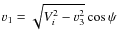
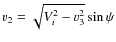
In the inertial frame centred on the star, (x,y,z), the acceleration a comet experiences from Galactic tides becomes
![$\displaystyle \Omega_{\rm G}^2 [(1-\delta)\cos(2\Omega_{\rm G} t)-\delta]x + \Omega_{\rm G}^2
(1-\delta)\sin(2\Omega_{\rm G} t)y$](/articles/aa/full_html/2010/08/aa14275-10/img23.png)
![$\displaystyle \Omega_{\rm G}^2 (1-\delta)\sin(2\Omega_{\rm G} t)x -\Omega_{\rm G}^2
[(1-\delta)\cos(2\Omega_{\rm G} t)+\delta]y,$](/articles/aa/full_html/2010/08/aa14275-10/img25.png)
![$\displaystyle [4\pi G \rho_{\rm G} - 2\Omega_{\rm G}^2 \delta]z.$](/articles/aa/full_html/2010/08/aa14275-10/img27.png)
At the solar orbit, R = 8 kpc,
2.1 Galactic potential and tidal field
To study the influence of the Galactic tides on the Oort cloud at various locations in the Galaxy, a model is needed for the potential of the Galaxy from which one can derive the Oort constants A and B and the matter densityThe potential consists of a component due to the bulge/stellar halo and inner core
![]() ,
the disc
,
the disc
![]() ,
and the dark halo
,
and the dark halo
![]() .
The core potential consists of two Plummer spheres, the disc is made up
of of three Miyamoto-Nagai components (Miyamoto & Nagai
1975), and the dark halo has a spherical, logarithmic form. From Flynn et al. (1996),
.
The core potential consists of two Plummer spheres, the disc is made up
of of three Miyamoto-Nagai components (Miyamoto & Nagai
1975), and the dark halo has a spherical, logarithmic form. From Flynn et al. (1996),
![$\displaystyle -\sum_{i=1}^3\frac{GM_{{\rm D}i}}{(R^2+[a_i+\sqrt{z^2+b^2}]^2)^{1/2}},$](/articles/aa/full_html/2010/08/aa14275-10/img38.png)

where
Table 1: Parameters used in the potential of the Galaxy.
![\begin{figure}
\par\includegraphics[angle=-90,width=9cm,clip]{14275fg01.eps}
\end{figure}](/articles/aa/full_html/2010/08/aa14275-10/img60.png)
|
Figure 1: Rotational velocity of our model Galaxy as a function of distance from the Galactic centre. The various components are indicated, and the thick solid line depicts the total value. |
| Open with DEXTER | |
![\begin{figure}
\par\includegraphics[angle=-90,width=9cm,clip]{14275fg02.eps}
\end{figure}](/articles/aa/full_html/2010/08/aa14275-10/img61.png)
|
Figure 2: Matter density in the midplane of our model Galaxy as a function of distance from the Galactic centre. The various components are indicated, and the thick solid line depicts the total value. |
| Open with DEXTER | |
From the relation
![]() between the potential and matter density, we find for the above potentials (Binney &
Tremaine 1987)
between the potential and matter density, we find for the above potentials (Binney &
Tremaine 1987)
|
|
= | 
|
|
| = | ![$\displaystyle \sum_{i=1}^3
\Bigl(\frac{b^2M_{{\rm D}i}}{4\pi}\Bigr)\frac{a_iR^2...
...})(a_i+\sqrt{
z^2+b^2})^2}
{[R^2+(a_i+\sqrt{z^2+b^2})^2]^{5/2}(z^2+b^2)^{3/2}},$](/articles/aa/full_html/2010/08/aa14275-10/img66.png)
|
(5) | |
| = | 
|
The density in the midplane is obtained by evaluating the above equations with z=0. At R=8 kpc,
The Oort constants A and B are related to the potential through (Binney & Tremaine 1987)
| A | = | 
|
|
| B | = | 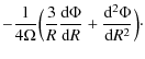
|
(6) |
The Oort constants, as well as
From all these relations, one can compute the strength of the vertical tide compared to the planar tides, TZ, i.e. the ratio of
![]() vs.
vs.
![]() and
and
![]() ,
which are obtained from Eq. (3). The value of TZ is calculated by averaging
the x and y tides over one Galactic rotation and making an approximation that x, y, and z have comparable magnitudes. We have
,
which are obtained from Eq. (3). The value of TZ is calculated by averaging
the x and y tides over one Galactic rotation and making an approximation that x, y, and z have comparable magnitudes. We have
| TZ | = | ![$\displaystyle \sqrt{2}\ddot{z}_{\rm G}\Bigl[\frac{1}{2\pi}\int
\limits_0^{2\pi/\Omega_{\rm G}}\ddot{x}_{\rm G}^2+\ddot{y}_{\rm G}^2~{\rm d}t\Bigr]^{-1/2}$](/articles/aa/full_html/2010/08/aa14275-10/img79.png)
|
|
|
(7) |
At 8 kpc, TZ=11.28. If
Now that we have a model for computing the tidal forces, we now turn to the passing Galactic field stars in the next section.
![\begin{figure}
\par\includegraphics[angle=-90,width=9cm,clip]{14275fg03.eps}\vspace*{2mm}
\end{figure}](/articles/aa/full_html/2010/08/aa14275-10/img84.png)
|
Figure 3:
Values of Oort constants A and |B| (top panel), the angular speed
|
| Open with DEXTER | |
![\begin{figure}
\par\includegraphics[angle=-90,width=9cm,clip]{14275fg04.eps}
\end{figure}](/articles/aa/full_html/2010/08/aa14275-10/img85.png)
|
Figure 4: Strength of z-tides versus radial tides for a symmetric (solid line) and asymmetric rotation curve (dashed line). |
| Open with DEXTER | |
![\begin{figure}
\par\includegraphics[angle=-90,width=9cm,clip]{14275fg05.eps}
\end{figure}](/articles/aa/full_html/2010/08/aa14275-10/img86.png)
|
Figure 5:
Radial and tangential velocity dispersions |
| Open with DEXTER | |
2.2 Passing stars
The issue of computing the action of passing stars on the Oort cloud contains several complexities, such as the correlation between age and velocity dispersion and the abundance of each spectral type as a function of Galactic distance. The latter is difficult to determine, while some attempts have been made to determine the first.
Lewis & Freeman (1989) have observed the velocity dispersion of the old disc as a function of the distance in the plane from the Galactic
centre. They were able to fit an exponential curve through their data for the radial and tangential velocity dispersions
(![]() and
and
![]() ,
respectively) with two different kinematic scale lengths. The best fit through their data is
,
respectively) with two different kinematic scale lengths. The best fit through their data is
While this gives a 1D velocity dispersion at R=8 kpc of 24.6 km s-1, similar to what is used by Heisler et al. (1987) and found by Garcia-Sanchez et al. (2001) for late spectral types, the 1D dispersion at 20 kpc is only
However, as argued by Evans & Collett (1993), the ratio of
![]() for the fit Lewis & Freeman (1989) used
is incorrect. Instead, Evans & Collett (1993) suggest a fit
for the fit Lewis & Freeman (1989) used
is incorrect. Instead, Evans & Collett (1993) suggest a fit
![]() ,
with b = 4.5 kpc and
,
with b = 4.5 kpc and
![]() km s-1. Unfortunately, Evans
& Collett (1993) do not give a fit for
km s-1. Unfortunately, Evans
& Collett (1993) do not give a fit for
![]() .
Attempting a similar fit to the data by Lewis & Freeman (1989) for
.
Attempting a similar fit to the data by Lewis & Freeman (1989) for
![]() yields poor results. The best fit we could find was a simple power law
with index -1.11 for a broad range of Galactic distance.
Bienaymé
& Séchaud (1997) obtain a very long kinematic scale length in the
solar neighbourhood, usually longer than 20 kpc, which they
attribute
to them having used more blue stars, whose kinematics are similar to
that of gas, implying that the scale length in these regions is
not well known. As a result, a power-law fit is probably okay. In the
top two panels of Fig. 5 we plot
yields poor results. The best fit we could find was a simple power law
with index -1.11 for a broad range of Galactic distance.
Bienaymé
& Séchaud (1997) obtain a very long kinematic scale length in the
solar neighbourhood, usually longer than 20 kpc, which they
attribute
to them having used more blue stars, whose kinematics are similar to
that of gas, implying that the scale length in these regions is
not well known. As a result, a power-law fit is probably okay. In the
top two panels of Fig. 5 we plot ![]() and
and
![]() of
Lewis & Freeman (1989) with the best fits mentioned earlier.
of
Lewis & Freeman (1989) with the best fits mentioned earlier.
If we assume that the above fits are representative of the reality in the range
![]() kpc, we can compute the 1D isotropic velocity
dispersion as
kpc, we can compute the 1D isotropic velocity
dispersion as
![]() .
Taking
.
Taking
![]() ,
which
is a reasonable assumption, and calculating the resulting values of
,
which
is a reasonable assumption, and calculating the resulting values of ![]() in the range we are interested in yields a best fit of
in the range we are interested in yields a best fit of
![]() km s-1. The value of
km s-1. The value of ![]() obtained this way from the data of Lewis & Freeman
(1989) and its best fit are depicted in the
bottom panel of Fig. 5, and yields
obtained this way from the data of Lewis & Freeman
(1989) and its best fit are depicted in the
bottom panel of Fig. 5, and yields
![]() km s-1 at 20 kpc, in reasonable agreement with the results of Rodionov
& Orlov (2008).
km s-1 at 20 kpc, in reasonable agreement with the results of Rodionov
& Orlov (2008).
The way the passing stars are implemented in our simulations follows.
We assume that the above change in velocity dispersion as a
function of Galactic distance is the same for all spectral types. In
other words, we assume that the relative increase or decrease in
velocity dispersion with Galactic distance is the same across all
spectral types. For example, the local 1D velocity dispersion
is about 25 km s-1 for M-dwarfs (Garcia-Sanchez et al. 2001). At 14 kpc this would be
![]() km s-1. For B-stars the velocity dispersion is about
8.5 km s-1 at 8 kpc, which becomes about 5 km s-1 at 14 kpc by this method.
km s-1. For B-stars the velocity dispersion is about
8.5 km s-1 at 8 kpc, which becomes about 5 km s-1 at 14 kpc by this method.
Now that we have an idea of how to model the passing Galactic field stars, in the next section we look at some relevant time scales that naturally enter into the problem.
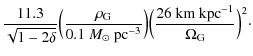
2.3 Time scales and relevant quantities
The tidal torquing time of the comet's pericentre due to the Galactic tide is given in Duncan et al. (1987) as
![]() .
Since the planar tides are not always small compared to the vertical tide, we cannot compute
.
Since the planar tides are not always small compared to the vertical tide, we cannot compute ![]() using only the
vertical tide. From Fouchard et al. (2005), who adds the contribution of the radial tides, we compute tq, in Myr, as
using only the
vertical tide. From Fouchard et al. (2005), who adds the contribution of the radial tides, we compute tq, in Myr, as
|
(9) |
where we used
|
(10) |
Here
For heavy planets the typical energy change a comet receives per
pericentre passage is much greater than the binding energy of a comet
in
the
cloud, so that only a low percentage of comets scattered by such
planets will land in the cloud. The semi-major axis at which this
becomes possible is computed from setting the tidal torquing time equal
to the orbital period (Duncan et al. 1987). The corresponding
minimum energy to which comets will be launched based on this time scale, using
![]() AU and
q=(9/8)ap (Brasser & Duncan
2008), is
AU and
q=(9/8)ap (Brasser & Duncan
2008), is
![$\displaystyle u_{\rm Cl} = 3.97 \times 10^{-5}
\Bigl[\zeta(\rho_{\rm G},\Omega_...
...r]^{2/7}\!\!
\Bigl(\frac{a_p}{5~{{\rm {AU}}}}\Bigr)^{1/7}\!\!{{\rm {AU}}}^{-1}.$](/articles/aa/full_html/2010/08/aa14275-10/img116.png)
For the potential that we used, a best fit through
where R is measured in kpc and the fit has errors less than 3%. Using ap = 5 AU at 2 kpc, the result is
For light planets, the comets diffuse towards the Oort cloud rather than being launched and are lifted at a semi-major axis
corresponding to where the diffusion time equals the tidal torquing time i.e. tq=td (Duncan
et al. 1987). Here the
diffusion time td is given by Duncan et al. (1987) as
|
(12) |
where
| |
= | ![$\displaystyle 0.011~\beta^{-4/3}
\Bigl[\zeta(\rho_{\rm G},\Omega_{\rm G})\Bigl(\frac{\rho_{\rm G}}{0.1~M_{\odot}~{{\rm {pc}}}^{-3}}\Bigr)\Bigr]^{2/3}$](/articles/aa/full_html/2010/08/aa14275-10/img128.png)
|
|
|
(13) |
Repeating the same exercise as before, the best fit to the factor
Using Neptune with
At R=20 kpc,
Taking t* = 5 Gyr, ap = 30 AU, and
Now that we know the time scales involved for massive and light planets to scatter the comets and in which part of the cloud these comets are most likely to end up, we inspect a few other time scales that naturally enter the problem. The first one is the half life for a comet in the cloud subjected to stellar perturbations, which is a measure of how long the comets can survive in the cloud, of how much the cloud wears down over time, and by proxy the total trapping efficiency of comets in the cloud. The second is the Kozai cycle time, which is a measure of how long the comet can stay in the cloud, before its pericentre reaches the planets again.
Bailey (1986), following Hut & Tremaine (1985), computes the half life for a comet in the Sun's Oort cloud subjected to perturbations
of
passing stars, which is given by (Brasser et al. 2008)
From Garcia-Sanchez et al. (2001), we have
|
(18) |
Using previous fitting relations and Bailey's (1986) formula, we get
|
(19) |
which, as one can see, increases exponentially with R for fixed a. The above result is a bit misleading since the behaviour of a with R is not taken into account.
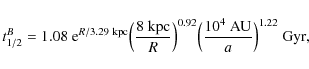
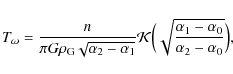
There is another times cale in this problem: the Kozai period of the comets, induced by the perturbations of the Galactic tide. The Kozai time measures how long it takes for the argument of pericentre of the comet to revolve one cycle (or, if the latter is librating, to perform one oscillation), and because the oscillations of the eccentricity and inclination of the comet are coupled to the evolution of the argument of pericentre (Kozai 1962), it is also the time it takes for the pericentre of the comet to perform one cycle and re-enter the planetary region. This time scale is a measure of how long a comet can be trapped in the cloud before it reaches the planetary region once again, provided it has not been stripped or has its trajectory reset by a passing star (Weissman 1980), and the stripping occurs on a time scale t1/2B. Once the pericentre of the comet re-enters the planetary region, it can be ejected by the planets.
Formally the Kozai period only exists when the radial tides do not,
because then the problem is integrable. However, if the strength
of radial tides is smaller than the vertical tide, then the Kozai
period can be computed approximately if the semi-major axis of the
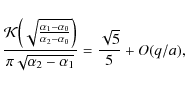
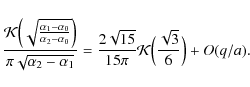
comet's orbit is not too large. Following Higuchi et al. (2007), the Kozai period becomes
|
(20) |
where n is the mean motion of the comet,
|
(21) |
while for
|
(22) |
Averaging between both these extremes, the period over the range
|
(23) |
Now that we have an understanding of the time scales involved and the parts of the cloud the comets end up as a function of the position and mass of the planet, we are ready to discuss the numerical simulations.
3 Method
We used a new code to perform the numerical simulations called SCATR (Symplectically-Corrected Adaptive Timestepping Routine) (Kaib et al. 2010), which is based on SWIFT's RMVS3 (Levison & Duncan 1994). SCATR is a modified RMVS3 to include passing stars and the influence of the Galactic tide (Levison et al. 2001; Dones et al. 2004). The major advantage of SCATR over RMVS3 is that it is able to use much longer time steps at large distances from the Sun.
For our simulations we used initial conditions similar to Dones et al. (2004) and Kaib & Quinn (2008). The giant planets are on their current orbits, after their instability at the time of the late heavy bombardment (Tsiganis et al. 2005; Gomes et al. 2005), and we used 2500 test particles to represent the comets, originally situated between 4 and 32 AU. We placed the Sun on orbits at 2, 4, 6, 8, 14 and 20 kpc from the Galactic centre, and the simulations were run for 4 Gyr. The criteria for removing comets were as follows: either they were hyperbolic or, if bound, farther than a certain distance from the Sun, which is computed below. A comet is deemed to be in the Oort cloud when its pericentre distance q>40 AU, its semi-major axis a>1000 AU, and its eccentricity e<1. All simulations for this study were run on the CRIMSON Beowulf cluster at OCA.
Table 2: Stellar data from Garcia-Sanchez et al. (2001).
The method of generating passing stars is based on a mixture of methods by Heisler et al. (1987) and by Rickman et al. (2008). Table 2,
which is taken from Garcia-Sanchez et al. (2001), shows the values of the mass mi, number density ni, and velocity dispersion
![]() for a large class of main-sequence stars in the solar neighbourhood. The velocity dispersion is taken to be the 1-dimensional
isotropic value and is obtained by dividing the values in Garcia-Sanchez et al. (2001) by
for a large class of main-sequence stars in the solar neighbourhood. The velocity dispersion is taken to be the 1-dimensional
isotropic value and is obtained by dividing the values in Garcia-Sanchez et al. (2001) by ![]() .
The outline follows.
.
The outline follows.
- Calculate the time of the mth stellar encounter tm, according to the method of Heisler et al. (1987). The
probability that the the next encounter happens at time t is given by
 ,
where f is the mean
encounter frequency of stars with impact parameters relative to the Sun shorter than some chosen maximum impact parameter
,
where f is the mean
encounter frequency of stars with impact parameters relative to the Sun shorter than some chosen maximum impact parameter
 .
From Heisler et al. (1987) we have
.
From Heisler et al. (1987) we have
(24)
where the sum is taken over stellar spectral types. Since both and ni change with Galactic distance, R, the value
of
needs to be adjusted to ensure that the passing stars are entered much farther away than the typical maximum apocentre
of a
comet's orbit (2 pc at the Sun's current location).
and ni change with Galactic distance, R, the value
of
needs to be adjusted to ensure that the passing stars are entered much farther away than the typical maximum apocentre
of a
comet's orbit (2 pc at the Sun's current location).
- Next we need to know the spectral type of the star. Again we use the method outlined in Heisler et al. (1987). Define
 and
and
 for any
  .
We then choose a uniform
random number between 0 and 1,
.
We then choose a uniform
random number between 0 and 1,  .
The star then has type i if
.
The star then has type i if
 .
Rickman et al. (2008) base the star's
type
on the encounter frequency of Garcia-Sanchez et al. (2001). While this method is as good as that of Heisler et al. (1987) we do not
know
the encounter frequencies at other Galactic distances, while we are able to compute estimates of ni and
.
Rickman et al. (2008) base the star's
type
on the encounter frequency of Garcia-Sanchez et al. (2001). While this method is as good as that of Heisler et al. (1987) we do not
know
the encounter frequencies at other Galactic distances, while we are able to compute estimates of ni and  (and
therefore
)
as outlined earlier.
(and
therefore
)
as outlined earlier.
- Next we choose the star's entry point on a sphere of radius
.
The position vector is generated as
 =
= 
(25)
where and
and  are chosen randomly with uniform distribution in the intervals
![$\cos \theta \in [-1,1]$](/articles/aa/full_html/2010/08/aa14275-10/img189.png) and
and
![$\phi \in
[0,2\pi]$](/articles/aa/full_html/2010/08/aa14275-10/img190.png) .
.
- The next step is to choose the magnitude of the velocity. For this we follow the outline of Rickman et al. (2008). The peculiar
velocity (
 )
of a star with respect to its local standard of rest is calculated from a spherical Maxwellian distribution as follows.
We compute three random numbers
)
of a star with respect to its local standard of rest is calculated from a spherical Maxwellian distribution as follows.
We compute three random numbers
 that have a Gaussian probability distribution with a mean of 0 and standard
deviation of 1. We use the formula
that have a Gaussian probability distribution with a mean of 0 and standard
deviation of 1. We use the formula
(26)
with l=5 where are random numbers between 0 and 1. The peculiar velocity of the star is then
 .
The magnitude of the star's heliocentric velocity is subsequently calculated by combining the vector
with the Sun's apex velocity
.
The magnitude of the star's heliocentric velocity is subsequently calculated by combining the vector
with the Sun's apex velocity  .
It should be noted that values for
only exist for the solar neighbourhood
(Table 2). We return to this issue shortly. We assume the two vectors are randomly oriented so that we have
.
It should be noted that values for
only exist for the solar neighbourhood
(Table 2). We return to this issue shortly. We assume the two vectors are randomly oriented so that we have
(27)
where is uniformly chosen between -1 and 1. Since the flux is dependent on velocity, the latter velocity needs to be modified.
Compute a high velocity for each spectral type, called V0i. Generate a random number
is uniformly chosen between -1 and 1. Since the flux is dependent on velocity, the latter velocity needs to be modified.
Compute a high velocity for each spectral type, called V0i. Generate a random number  .
Then, if
.
Then, if
 ,
keep the
value of Vi, otherwise recompute it according to the above until the condition for
is fulfilled. We chose
,
keep the
value of Vi, otherwise recompute it according to the above until the condition for
is fulfilled. We chose
 .
.
- Last, we need to know the components of the velocity vector of the star. Define v3 as the component anti-parallel to the radius
vector and v1 and v2 as the components orthogonal to it. Then we have
 where
is a random number between 0
and 1, and
where
is a random number between 0
and 1, and
 and
and
 ,
where
,
where
 .
The components of the
velocity are then
.
The components of the
velocity are then
where the same and
that were used for the radius vector need to be inserted.
and
that were used for the radius vector need to be inserted.
To estimate the value of
![]() ,
we proceed along the lines of Antonov & Latyshev (1972) by studying the zero-velocity
curves around the Sun. According to Antonov & Latyshev (1972), the Jacobi constant for the system consisting of a comet orbiting the Sun in
the co-ordinate system erected in Sect. 2 is
,
we proceed along the lines of Antonov & Latyshev (1972) by studying the zero-velocity
curves around the Sun. According to Antonov & Latyshev (1972), the Jacobi constant for the system consisting of a comet orbiting the Sun in
the co-ordinate system erected in Sect. 2 is
|
(28) |
where C is the ``third Oort constant'', given by

|
(29) |
and is a measure of the vertical frequency of the Sun's motion. After computing it, a best fit for
| xc | = | 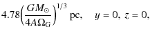
|
|
| yc | = | (30) | |
| zc | = | ![$\displaystyle 4.78\frac{(GM_{\odot})^{1/3}}{C}\Bigl[\Psi(A,C,\Omega_{\rm G})-\frac{(4A\Omega_{\rm G})^{
1/3}}{\Psi(A,C,\Omega_{\rm G})}\Bigr] ~ {{\rm {pc}}},$](/articles/aa/full_html/2010/08/aa14275-10/img225.png)
|
|
where
![\begin{figure}
\par\includegraphics[angle=-90,width=9cm,clip]{14275fg06.eps}
\end{figure}](/articles/aa/full_html/2010/08/aa14275-10/img230.png)
|
Figure 6: Values of xc (solid line), yc (long dash), and zc (short dash) as a function of distance to the Galactic centre. |
| Open with DEXTER | |
![\begin{figure}
\par\includegraphics[angle=-90,width=9cm,clip]{14275fg07.eps}
\end{figure}](/articles/aa/full_html/2010/08/aa14275-10/img231.png)
|
Figure 7: Inner edge of the Oort cloud as a function of Galactic distance. Bullets are the 5% mark, error bars depict 1% and 10% levels. |
| Open with DEXTER | |
4 Results of numerical simulations
In this section the results of our numerical simulations are described. We are interested in the following issues: the internal structure of the cloud, the formation efficiency, the formation duration, and the extent and size of the cloud.
We first focus on the size and extent of the cloud. In Fig. 7 we plot the semi-major axis of the inner edge of the clouds as a
function of Galactic distance. The line denotes the analytical result of Eq. (15) where we used ap=25 AU,
![]()
![]() ,
and
,
and ![]() .
The bullets denote the value of semi-major axis inside of which 5% of
the comets reside. The upper
and lower marks of the error bars denote the same for 1% and 10%. As
one can see, the analytical result follows the bullets rather
well. This leads us to conclude that, generally, the analytic result
can be
used. The next figure, Fig. 8,
plots the cumulative distribution in semi-major axis of Oort clouds at
2 (leftmost line), 8,
14,
and 20 kpc (rightmost line). These distributions show the size and
extent of the clouds. The distributions shift towards higher values
of
semi-major axis with increasing Galactic distance, as expected.
Additionally, the extent of the cloud decreases with increasing
distance.
At 2 kpc the ratio between the inner and outer edges is
approximately 30, while at 20 kpc this ratio is close to 8. Thus,
closer to the
Galactic centre, the comets are spread over a winder range of binding
energies.
.
The bullets denote the value of semi-major axis inside of which 5% of
the comets reside. The upper
and lower marks of the error bars denote the same for 1% and 10%. As
one can see, the analytical result follows the bullets rather
well. This leads us to conclude that, generally, the analytic result
can be
used. The next figure, Fig. 8,
plots the cumulative distribution in semi-major axis of Oort clouds at
2 (leftmost line), 8,
14,
and 20 kpc (rightmost line). These distributions show the size and
extent of the clouds. The distributions shift towards higher values
of
semi-major axis with increasing Galactic distance, as expected.
Additionally, the extent of the cloud decreases with increasing
distance.
At 2 kpc the ratio between the inner and outer edges is
approximately 30, while at 20 kpc this ratio is close to 8. Thus,
closer to the
Galactic centre, the comets are spread over a winder range of binding
energies.
We now turn to the matter of the formation efficiency of the cloud. We depict this efficiency at various Galactic distances in
Fig. 9.
The top panel depicts the efficiency of depositing the comets in the
Oort cloud after 4 Gyr, while the bottom panel shows
the efficiency of depositing comets assuming that no subsequent decay
takes place; i.e., all the comets that make it to the cloud are
deposited there at the same time, and there is no subsequent erosion
caused by the passing stars and the Galactic tide. The bottom panel
should only be used as an indicator of a theoretical upper limit to the
efficiency. It is surprising that the top panel shows small
deviations in the overall efficiency as a function of Galactic
distance. The difference is more pronounced in the lower panel but this
is to
be expected: the density
![]() is higher closer to the Galactic centre so that comets are trapped
closer to the
Sun and thus, in principle, have a higher efficiency. That the
efficiency after 4 Gyr is more or less independent of Galactic
distance implies that there is more wearing down of the cloud in the
inner parts of the Galaxy, even though the comets are
closer to the Sun. The low trapping efficiencies at short Galactic
distance do not bode well for explaining the LPC flux. We return to
this in the next section.
is higher closer to the Galactic centre so that comets are trapped
closer to the
Sun and thus, in principle, have a higher efficiency. That the
efficiency after 4 Gyr is more or less independent of Galactic
distance implies that there is more wearing down of the cloud in the
inner parts of the Galaxy, even though the comets are
closer to the Sun. The low trapping efficiencies at short Galactic
distance do not bode well for explaining the LPC flux. We return to
this in the next section.
A good measure of the internal structure and distribution of the cloud is to calculate its density profile, n(a), which measures
the volume density of comets with semi-major axis between a and
![]() ,
i.e.,
,
i.e.,
![]() .
For most clouds n(a)is a power law, i.e.,
.
For most clouds n(a)is a power law, i.e.,
![]() .
Figure 10
depicts a few such density profiles for clouds at various Galactic
distances: the
top-left panel is for the cloud at 2 kpc, the top-right panel is
at 8 kpc, the bottom-left panel refers to 14 kpc, and the
last
panel refers to the cloud at 20 kpc. The line shows the best fit,
all of which are power laws. The index
.
Figure 10
depicts a few such density profiles for clouds at various Galactic
distances: the
top-left panel is for the cloud at 2 kpc, the top-right panel is
at 8 kpc, the bottom-left panel refers to 14 kpc, and the
last
panel refers to the cloud at 20 kpc. The line shows the best fit,
all of which are power laws. The index ![]() ranges from -2.7 at 14 kpc
to -3.3 for the outer parts of the cloud at 20 kpc. The inner part at 20 kpc can be fit by
ranges from -2.7 at 14 kpc
to -3.3 for the outer parts of the cloud at 20 kpc. The inner part at 20 kpc can be fit by
![]() .
Dones et al. (2004) has already reported that the inner parts of the Oort cloud have a flat density distribution, which is clearly visible
in
the last panel.
.
Dones et al. (2004) has already reported that the inner parts of the Oort cloud have a flat density distribution, which is clearly visible
in
the last panel.
![\begin{figure}
\par\includegraphics[angle=-90,width=9cm,clip]{14275fg08.eps}
\end{figure}](/articles/aa/full_html/2010/08/aa14275-10/img238.png)
|
Figure 8: Cumulative distribution in semi-major axis for clouds at 2, 8, 14, and 20 kpc. |
| Open with DEXTER | |
![\begin{figure}
\par\includegraphics[angle=-90,width=9cm,clip]{14275fg09.eps}
\end{figure}](/articles/aa/full_html/2010/08/aa14275-10/img239.png)
|
Figure 9: Top: Percentage of comets after 4 Gyr in Oort clouds generated by using the giant planets of our Solar System on their current orbits. Bottom: Efficiency the Oort clouds would have if assuming no subsequent erosion. |
| Open with DEXTER | |
![\begin{figure}
\par\includegraphics[angle=-90,width=9cm,clip]{14275fg10.eps}
\end{figure}](/articles/aa/full_html/2010/08/aa14275-10/img240.png)
|
Figure 10: Density profiles of some Oort clouds as a function of a. Top-left panel is at 2 kpc, top-right at 8 kpc, bottom-left at 14 kpc, and bottom-right at 20 kpc. |
| Open with DEXTER | |
It is interesting to compare this result with earlier simulations. Dones et al. (2004) finds
![]() for the whole Oort cloud,
though they also employ a two-stage power law that gives a steeper slope in the outer parts (-3.7). For the cloud at 8 kpc,
we have
for the whole Oort cloud,
though they also employ a two-stage power law that gives a steeper slope in the outer parts (-3.7). For the cloud at 8 kpc,
we have
![]() ,
similar to what Dones et al. (2004) find. This is to be expected since the simulations presented here are
identical to those of Dones et al. (2004), so it is encouraging that we get the same result, and it proves that the slightly
different values of the Oort constants A and B, as well as the increased stellar encounter speeds, make little difference for the final
result.
,
similar to what Dones et al. (2004) find. This is to be expected since the simulations presented here are
identical to those of Dones et al. (2004), so it is encouraging that we get the same result, and it proves that the slightly
different values of the Oort constants A and B, as well as the increased stellar encounter speeds, make little difference for the final
result.
Another measure to identify the inner structure of the cloud is to plot the mean eccentricity
![]() and ecliptic
inclination
and ecliptic
inclination
![]() ,
of objects in certain parts of the cloud. These quantities have been depicted in Fig. 11, which
shows the values of
,
of objects in certain parts of the cloud. These quantities have been depicted in Fig. 11, which
shows the values of
![]() and
and
![]() at the 10th (bullets), 50th (open circles) and 90th (triangles)
percentiles in a as a function of Galactic distance. The straight lines at
at the 10th (bullets), 50th (open circles) and 90th (triangles)
percentiles in a as a function of Galactic distance. The straight lines at
![]() and
and
![]() are values for a system that is isotropic and in virial equilibrium. The data was gathered as follows: comets that are
in the cloud were sorted according to semi-major axis, which yields the cumulative distribution, F(a). For the data points corresponding
to the 10th percentile, we averaged the eccentricity or inclination of comets with semi-major axes between F(0.05) and
F(0.15).
We performed similar methods for the other data points. The inner
regions and around the median distance the clouds are always more
eccentric than the virial value, while the comets are more circular
when farther than the median distance. Regarding the
inclinations, the inner
parts are always prograde, similar to what Dones et al. (2004) and Kaib & Quinn (2008) find. Around the median, the clouds are as good as
isotropic, but at large distances from the Sun the clouds are predominantly prograde yet again.
are values for a system that is isotropic and in virial equilibrium. The data was gathered as follows: comets that are
in the cloud were sorted according to semi-major axis, which yields the cumulative distribution, F(a). For the data points corresponding
to the 10th percentile, we averaged the eccentricity or inclination of comets with semi-major axes between F(0.05) and
F(0.15).
We performed similar methods for the other data points. The inner
regions and around the median distance the clouds are always more
eccentric than the virial value, while the comets are more circular
when farther than the median distance. Regarding the
inclinations, the inner
parts are always prograde, similar to what Dones et al. (2004) and Kaib & Quinn (2008) find. Around the median, the clouds are as good as
isotropic, but at large distances from the Sun the clouds are predominantly prograde yet again.
Some of the effects depicted in Fig. 11 are also visible when plotting the comets in a-q space at the end of the simulations. Figure 12 shows a sample of Oort clouds at the end of the simulations. The top-left panel depicts the cloud located at 2 kpc from the Galactic centre, the top-right panel is at 8 kpc, the bottom-left panel refers to 14 kpc, and the bottom-right panel refers to 20 kpc. The structures are different at various distances. Two effects are clearly visible. The first is that in each panel where the distance to the Galactic centre is farther than the previous one, the distance of the cloud to the Sun increases, as we showed earlier. The second effect pertains to the distribution in q: these values are systematically higher in proportion to the semi-major axis at the outer edges of the cloud, while the values of q span a much wider range around the median. Of course, near the inner edge, the range in q is limited because of lower values of the semi-major axis and because the comets have not had the time to complete one Kozai cycle.
One last question one could ask is the formation time of the cloud, especially when comparing the formation time with the orbital period of the Sun around the Galactic centre. One could envision that, if the formation time is comparable to the orbital period of the Sun, the cloud could have encountered several spiral arms, depending on how close the Sun orbits the co-rotation radius, and these encounters might have caused the Sun to migrate (Sellwood & Binney 2002). In Fig. 13 we plot the cumulative time for comets the reach the cloud, for clouds at 2, 8, 14, and 20 kpc (left to right, respectively). As one can see, the formation time increases with increasing Galactic distance, which is caused by the planets having to scatter the comets onto larger orbits before the tides can lift them into the cloud. The fraction of comets deposited into the cloud scales approximately logarithmic with time. The median formation time of the cloud ranges from 50 Myr at 2 kpc to 150 Myr at 20 kpc, which is shorter than or comparable to the orbital period of the Sun at most Galactic distances. At 8 kpc, over 70% of the comets that survive after 4 Gyr in the cloud are already in the cloud after one Galactic orbit so that during the formation process the Sun can probably be considered to be on a fixed orbit. It is only during the subsequent evolution of the cloud after the formation process that the migration of the Sun becomes important. We discuss this in the next section.
![\begin{figure}
\par\includegraphics[angle=-90,width=9cm,clip]{14275fg11.eps}
\end{figure}](/articles/aa/full_html/2010/08/aa14275-10/img248.png)
|
Figure 11:
Values of
|
| Open with DEXTER | |
![\begin{figure}
\par\includegraphics[angle=-90,width=9cm,clip]{14275fg12.eps}
\end{figure}](/articles/aa/full_html/2010/08/aa14275-10/img249.png)
|
Figure 12: Some sample Oort clouds in a-q space at the end of the simulations. Top left: 2 kpc. Top right: 8 kpc. Bottom left: 14 kpc. Bottom right: 20 kpc. |
| Open with DEXTER | |
![\begin{figure}
\par\includegraphics[angle=-90,width=9cm,clip]{14275fg13.eps}
\end{figure}](/articles/aa/full_html/2010/08/aa14275-10/img250.png)
|
Figure 13: Cumulative time of depositing comets in the cloud for Galactic distances of 2, 8, 14, and 20 kpc (left to right). |
| Open with DEXTER | |
5 Discussion and implications
The results presented in the previous section are to be expected based on earlier work of Dones et al. (2004) and Kaib & Quinn (2008), as well as the theory presented in section 2. Nontheless, it contains a few surprises that we believe should be discussed. However, first there are a few other points that we want to clarify.
The first issue is that the formation efficiency is more or less the same for most Galactic distances: 3% ![]() 1%. The second issue
deals
with solar migration within the Galaxy, and needs further discussion. Sellwood & Binney (2002)
have demonstrated that solar
encounters with spiral arms can force the Sun to migrate significantly
while keeping its orbit nearly circular. The current position of the
Sun is
consistent with a formation between 4 and 12 kpc. In the
simulations presented here we kept the Sun at the same distance from
the Galactic
centre for 4 Gyr. Since it is likely that the Sun has migrated
during that time, the results of these simulations should be viewed as
a
proof of concept rather than as indicative of the current Oort cloud
and as representative of its population. A way that migration will
affect the structure of the Oort cloud can be understood from the
following example in which we assume that the Oort cloud formed in two
stages as outlined in Brasser (2008).
Suppose that during the time of the late heavy bombardment - a phase of
intense bombardment of
the terrestrial planets, most likely caused by a dynamical instability
of the outer planets approximately 600 Myr after the formation of the
giant planets (Tsiganis et al. 2005; Gomes et al. 2005)
- the Sun was closer to
the Galactic centre than it is today, at 4 kpc or so. During the
time of the late heavy bombardment, a lot of material very
quickly becomes available for the giant planets to scatter (Gomes
et al. 2005).
From the results presented in the previous
section, it appears that most comets are in the Oort cloud after nearly
a hundred million years and that there is subsequently an
exponentially-decreasing flux of comets reaching the cloud until the
end of the simulations. This can be understood from Fig. 13:
the cumulative distribution is more or less linear as a function of
1%. The second issue
deals
with solar migration within the Galaxy, and needs further discussion. Sellwood & Binney (2002)
have demonstrated that solar
encounters with spiral arms can force the Sun to migrate significantly
while keeping its orbit nearly circular. The current position of the
Sun is
consistent with a formation between 4 and 12 kpc. In the
simulations presented here we kept the Sun at the same distance from
the Galactic
centre for 4 Gyr. Since it is likely that the Sun has migrated
during that time, the results of these simulations should be viewed as
a
proof of concept rather than as indicative of the current Oort cloud
and as representative of its population. A way that migration will
affect the structure of the Oort cloud can be understood from the
following example in which we assume that the Oort cloud formed in two
stages as outlined in Brasser (2008).
Suppose that during the time of the late heavy bombardment - a phase of
intense bombardment of
the terrestrial planets, most likely caused by a dynamical instability
of the outer planets approximately 600 Myr after the formation of the
giant planets (Tsiganis et al. 2005; Gomes et al. 2005)
- the Sun was closer to
the Galactic centre than it is today, at 4 kpc or so. During the
time of the late heavy bombardment, a lot of material very
quickly becomes available for the giant planets to scatter (Gomes
et al. 2005).
From the results presented in the previous
section, it appears that most comets are in the Oort cloud after nearly
a hundred million years and that there is subsequently an
exponentially-decreasing flux of comets reaching the cloud until the
end of the simulations. This can be understood from Fig. 13:
the cumulative distribution is more or less linear as a function of ![]() ,
so that a histogram of number of comets deposited vs
,
so that a histogram of number of comets deposited vs ![]() is
more or less flat, thus indicating a logarithmic increase in the
number of comets being deposited in the cloud. In the inner parts of
the Galaxy the flux of stellar encounters and short Kozai cycle time
cause the Oort cloud to erode very quickly. However, the majority of
comets can be saved if the Sun were to migrate outwards shortly after
the late heavy bombardment so that the retention of comets will be
higher than closer to the Galactic centre. This would help the scenario
of Kaib & Quinn (2009),
because when the Sun is at 4 kpc
most of the comets get deposited in the inner cloud, where they argue
most of the LPCs could originate from. In other words, the potential
exists for creating a more massive inner Oort cloud than in the
scenario of Dones et al. (2004) and Kaib & Quinn (2008)
if the
circumstances are just lucky enough. Alternatively, if the Sun formed
much farther out, all of the comets would have been deposited in the
outer cloud and the problem of the flux of LPCs need not bother with a
possible inner Oort cloud population. Of course, in that case the low
formation efficiency makes it difficult to reconcile the LPC flux with
the remaining mass of the primordial solar nebula, which became fully
destabilised during the late heavy bombardment.
is
more or less flat, thus indicating a logarithmic increase in the
number of comets being deposited in the cloud. In the inner parts of
the Galaxy the flux of stellar encounters and short Kozai cycle time
cause the Oort cloud to erode very quickly. However, the majority of
comets can be saved if the Sun were to migrate outwards shortly after
the late heavy bombardment so that the retention of comets will be
higher than closer to the Galactic centre. This would help the scenario
of Kaib & Quinn (2009),
because when the Sun is at 4 kpc
most of the comets get deposited in the inner cloud, where they argue
most of the LPCs could originate from. In other words, the potential
exists for creating a more massive inner Oort cloud than in the
scenario of Dones et al. (2004) and Kaib & Quinn (2008)
if the
circumstances are just lucky enough. Alternatively, if the Sun formed
much farther out, all of the comets would have been deposited in the
outer cloud and the problem of the flux of LPCs need not bother with a
possible inner Oort cloud population. Of course, in that case the low
formation efficiency makes it difficult to reconcile the LPC flux with
the remaining mass of the primordial solar nebula, which became fully
destabilised during the late heavy bombardment.
Unfortunately, it is very unlikely that solar migration will save the day if the following is correct. Kaib & Quinn (2009) argue that
there are approximately
![]() km-sized comets in the whole Oort cloud. Morbidelli
et al. (2009) state that there are
approximately 1012 km-sized
bodies in the trans-Neptunian disc before the late heavy bombardment.
To get the required Oort
cloud population, we need a trapping efficiency of approximately 20%
after 4 Gyr, which is much higher than attained in any of the
simulations presented in this work. One could argue that the first Oort
cloud, which was formed when the Sun was still in its birth cluster,
could supply the necessary flux of LPCs in the manner explained by Kaib
& Quinn (2009). The formation efficiency of that first Oort cloud
is approximately 10% (Brasser et al. 2006; Kaib & Quinn 2008), which might be just enough to explain the LPC flux. However, if
90377 Sedna formed by the same mechanism, then most
of the comets in this first cloud are inside 5000 AU, where the Kaib & Quinn (2009)
mechanism cannot operate. Additionally, the gas
drag from the solar nebula prevents km-sized comets from being
scattered in the early age of the Solar System (Brasser et al. 2007),
so
that the fist Oort cloud would only consist of large bodies or would be
altogether empty. Indeed, no Sedna analogues have been found thus
far
(Schwamb et al. 2009), which begs the question of whether or not it is a fluke, i.e., a 2
km-sized comets in the whole Oort cloud. Morbidelli
et al. (2009) state that there are
approximately 1012 km-sized
bodies in the trans-Neptunian disc before the late heavy bombardment.
To get the required Oort
cloud population, we need a trapping efficiency of approximately 20%
after 4 Gyr, which is much higher than attained in any of the
simulations presented in this work. One could argue that the first Oort
cloud, which was formed when the Sun was still in its birth cluster,
could supply the necessary flux of LPCs in the manner explained by Kaib
& Quinn (2009). The formation efficiency of that first Oort cloud
is approximately 10% (Brasser et al. 2006; Kaib & Quinn 2008), which might be just enough to explain the LPC flux. However, if
90377 Sedna formed by the same mechanism, then most
of the comets in this first cloud are inside 5000 AU, where the Kaib & Quinn (2009)
mechanism cannot operate. Additionally, the gas
drag from the solar nebula prevents km-sized comets from being
scattered in the early age of the Solar System (Brasser et al. 2007),
so
that the fist Oort cloud would only consist of large bodies or would be
altogether empty. Indeed, no Sedna analogues have been found thus
far
(Schwamb et al. 2009), which begs the question of whether or not it is a fluke, i.e., a 2![]() - or 3
- or 3![]() event where an
unlikely close stellar passage with the Sun occurred while it was still
in its birth cluster. Last, the observed population ratio
between the Oort cloud and the scattered disc
(defined as comets having
event where an
unlikely close stellar passage with the Sun occurred while it was still
in its birth cluster. Last, the observed population ratio
between the Oort cloud and the scattered disc
(defined as comets having
![]() AU and a > 40 AU) is approximately 1000:1 (Duncan & Levison 1997; Levison & Duncan 1997;
Levison et al 2008), while simulations tend to yield a 5:1 ratio (Kaib & Quinn 2008) to 20:1 (Dones et al. 2004).
We find a population
ratio between 15-25:1 for our simulations presented here, with no clear
correlation between this ratio and Galactic distance. Unfortunately
it is much less than the observed value and is a severe shortcoming of
these simulations (Dones et al. 2004; Kaib & Quinn 2008).
Apparently changing the strength of the tides does not alter this ratio.
AU and a > 40 AU) is approximately 1000:1 (Duncan & Levison 1997; Levison & Duncan 1997;
Levison et al 2008), while simulations tend to yield a 5:1 ratio (Kaib & Quinn 2008) to 20:1 (Dones et al. 2004).
We find a population
ratio between 15-25:1 for our simulations presented here, with no clear
correlation between this ratio and Galactic distance. Unfortunately
it is much less than the observed value and is a severe shortcoming of
these simulations (Dones et al. 2004; Kaib & Quinn 2008).
Apparently changing the strength of the tides does not alter this ratio.
We should emphasise, though, that the above numbers are fraught with large uncertainties. The number of comets in the cloud is
inferred from
the LPC flux, which currently stands at
approximately 2-3 comets per year with q<4 AU
(Francis 2005).
An error of 1 comet per year on
either side increases the number of comets in the cloud appropriately,
hence the necessary formation efficiency, with a lower LPC flux
better supporting our models. Another uncertain parameter is the number
of objects in the scattered disc. Even though dynamical models
based on the flux of Jupiter-family comets yield approximately
![]() km-sized bodies, the precise number depends on the size
distribution. For the Kuiper belt, the best fit is a two-stage power law (Bernstein et al. 2004, Fraser & Kavelaars 2009; Fuentes &
Holman 2008; Fuentes et al. 2009) with a differential size distribution
km-sized bodies, the precise number depends on the size
distribution. For the Kuiper belt, the best fit is a two-stage power law (Bernstein et al. 2004, Fraser & Kavelaars 2009; Fuentes &
Holman 2008; Fuentes et al. 2009) with a differential size distribution
![]() where
where
![]() for objects
with diameters
for objects
with diameters
![]() km, and
km, and
![]() for smaller objects. Taking
for smaller objects. Taking
![]() and using the fact that there are
approximately 105 objects in the scattered disc with D > 50 km
(Levison et al. 2008) gives us approximately
and using the fact that there are
approximately 105 objects in the scattered disc with D > 50 km
(Levison et al. 2008) gives us approximately
![]() km-sized
bodies in the scattered disc; this can be pushed to
km-sized
bodies in the scattered disc; this can be pushed to
![]() objects when using
objects when using
![]() .
The latter number is still two
orders of magnitude lower than the inferred population of the Oort
cloud. However, the parameter with the largest uncertainty is the
conversion from absolute magnitude to diameter. For scattered disc
objects, this involves the albedo but for comets the conversion is much
poorer because the coma hides the nucleus. Therefore, we may be mislead
thinking that the flux of LPCs of 2-3 comets per year is for
km-sized objects while these bodies might, in fact, be a lot smaller.
Only if we underestimate the sizes of Oort cloud comets by at least
an order of magnitude do the two population ratios begin to agree, but
this seems unlikely. Therefore, in light of the above problems, we
tend to rule out the formation of the Oort cloud by this mechanism. The
only alternative mechanism that can explain the high population
ratios we can think of is the trapping of comets while the Sun was in
its birth cluster, provided the other stars could scatter the comets
out and not be hindered by gas drag. The trapping scenario is being
explored (Levison et al. 2010).
.
The latter number is still two
orders of magnitude lower than the inferred population of the Oort
cloud. However, the parameter with the largest uncertainty is the
conversion from absolute magnitude to diameter. For scattered disc
objects, this involves the albedo but for comets the conversion is much
poorer because the coma hides the nucleus. Therefore, we may be mislead
thinking that the flux of LPCs of 2-3 comets per year is for
km-sized objects while these bodies might, in fact, be a lot smaller.
Only if we underestimate the sizes of Oort cloud comets by at least
an order of magnitude do the two population ratios begin to agree, but
this seems unlikely. Therefore, in light of the above problems, we
tend to rule out the formation of the Oort cloud by this mechanism. The
only alternative mechanism that can explain the high population
ratios we can think of is the trapping of comets while the Sun was in
its birth cluster, provided the other stars could scatter the comets
out and not be hindered by gas drag. The trapping scenario is being
explored (Levison et al. 2010).
6 Summary and conclusions
We performed numerical simulations of the formation and evolution of the Oort cloud with the Sun orbiting the Galactic centre at a distance ranging from 2 kpc to 20 kpc. We used an up-to-date model for the Galactic potential and computed the solar orbit, matter density and other parameters from it that are needed to calculate the Galactic perturbations on the comets in the cloud. We used the observational results of Lewis & Freeman (1989) to compute the 1D velocity dispersion of stars at various Galactic distances, from which we constructed a method of computing the action of these passing stars on the Oort cloud in our integrator called SCATR (Kaib et al. 2010) based on methods by Heisler et al. (1987) and Rickman et al. (2008).
We have demonstrated that the Oort cloud can readily form in the other parts of the Galaxy. For the clouds that were
generated,
we established that the inner edge of the cloud - defined as the 5% mark in the cumulative semi-major axis distribution -
fits approximately with the theory of Eq. (15).
The clouds tend to have a flattened, very eccentric inner part, which
is
caused by the tides and stars torquing the comets very slowly, and a
mostly isotropic middle and outer part, with mean eccentricity fairly
close to the virial value of 2-1/2 and mean ecliptic inclination close to 90![]() .
However, the eccentricities close to the outer
edge of the cloud tend to be below the virial value, and the ecliptic inclinations favour prograde motion.
.
However, the eccentricities close to the outer
edge of the cloud tend to be below the virial value, and the ecliptic inclinations favour prograde motion.
The efficiency of trapping comets in the cloud after 4 Gyr ranges from 2% at 2 kpc to 4.5% at 8 kpc and is more or less independent of the distance to the Galactic centre. The difference in efficiency between a cloud at 2 kpc and one at 8 kpc is caused by the stronger erosion of the cloud closer to the Galactic centre, owing to the higher density of stars in these regions and the shorter Kozai cycle. Therefore, the efficiency cannot be used to trace a possible migration of the Sun in the Galaxy. We conclude that this efficiency is not high enough to explain the current flux of LPCs, even if the Sun was originally closer to the Galactic centre and subsequently migrated outwards. In addition, the population ratio between the Oort cloud and the scattered disc is lower than the observed value by approximately two orders of magnitude. Therefore, assuming that gas drag prevents the formation of an Oort cloud during the cluster stage, the only viable alternative to explaining the number of comets in the Oort cloud is through the trapping of interstellar comets while the Sun was in its putative birth cluster.
AcknowledgementsWe wish to thank Chris Flynn for very helpful discussions of the Galactic potential and the stellar velocity dispersion during the early stages of this study. We also thank Alessandro Morbidelli and an anonymous reviewer for helpful comments. R.B. thanks Germany's Helmholtz Alliance for financial support through their `Planetary evolution and Life' programme. A.H. thanks the Japan Society for the Promotion of Science for supporting this work. N.A.K. is financed by a NASA Earth and Space Science Fellowship.
References
- Antonov, V. A., & Latyshev, I. N. 1972, IAUS, 45, 341 [NASA ADS] [Google Scholar]
- Bailey, M. E.1986, MNRAS, 218, 1 [NASA ADS] [Google Scholar]
- Bernstein, G. M., Trilling, D. E., Allen, R. L., et al. 2004, AJ, 128, 1364 [NASA ADS] [CrossRef] [Google Scholar]
- Binney, J., & Tremaine, S. 1987, Galactic Dynamics (Princeton, NJ, USA: Princeton University Press) [Google Scholar]
- Brasser, R. 2008, A&A, 492, 251 [NASA ADS] [CrossRef] [EDP Sciences] [Google Scholar]
- Brasser, R., & Duncan, M. J. 2008, CeMDA, 100, 1 [NASA ADS] [CrossRef] [Google Scholar]
- Brasser, R., Duncan, M. J., & Levison, H. F. 2006, Icarus, 184, 59. [NASA ADS] [CrossRef] [Google Scholar]
- Brasser, R., Duncan, M. J., & Levison, H. F. 2007, Icarus, 191, 413 [NASA ADS] [CrossRef] [Google Scholar]
- Brasser, R., Duncan, M. J., & Levison, H. F. 2008, Icarus, 196, 274 [NASA ADS] [CrossRef] [Google Scholar]
- Demers, S., & Battinelli, P. 2007, A&A, 473, 143 [NASA ADS] [CrossRef] [EDP Sciences] [Google Scholar]
- Dones, L., Weissman, P. R., Levison, H .F., & Duncan, M. J. 2004, Oort cloud formation and dynamics. In: Star Formation in the Interstellar Medium, ed. Johnstone, D., Adams, F. C., Lin, D. N. C. Neufeld, D. A., & Ostriker, E. C. (San Francisco), ASPC, 324, 371 [Google Scholar]
- Duncan, M. J., & Levison, H. F. 1997, Science, 276, 1670 [NASA ADS] [CrossRef] [PubMed] [Google Scholar]
- Duncan, M., Quinn, T., & Tremaine, S. 1987, AJ, 94, 1330 [NASA ADS] [CrossRef] [Google Scholar]
- Evans, N. W., & Collet, J. L. 1993, MNRAS, 264, 353 [NASA ADS] [Google Scholar]
- Everhart, E. 1968, AJ, 73, 1039 [NASA ADS] [CrossRef] [Google Scholar]
- Fernández, J. A. 2002, ESASP, 500, 303 [Google Scholar]
- Flynn, C., Sommer-Larsen, J., & Christensen, P. R. 1996, MNRAS, 281, 1027 [NASA ADS] [CrossRef] [Google Scholar]
- Francis, P. J. 2005, ApJ, 635, 1348 [NASA ADS] [CrossRef] [Google Scholar]
- Fouchard, M., Froeschlé, Ch., Matese, J. J., & Valsecchi, G. 2005. CeMDA, 93, 229 [Google Scholar]
- Fraser, W. C., & Kavelaars, J. J. 2009, AJ, 137, 72 [NASA ADS] [CrossRef] [Google Scholar]
- Fuentes, C. I., & Holman, M. J. 2008. AJ, 136, 83 [Google Scholar]
- Fuentes, C. I., George, M. R., & Holman, M. J. 2009, ApJ, 696, 91 [NASA ADS] [CrossRef] [Google Scholar]
- García-Sánchez, J., Weissman, P. R., Preston, R. A., et al. 2001. A&A, 379, 634 [Google Scholar]
- Gomes, R., Levison, H., Tsiganis, K., & Morbidelli, A. 2005, Nature, 435, 466 [NASA ADS] [CrossRef] [PubMed] [Google Scholar]
- Heisler, J., & Tremaine, S. 1986, Icarus, 65, 13 [NASA ADS] [CrossRef] [Google Scholar]
- Heisler, J., Tremaine, S., & Alcock, C. 1987, Icarus, 70, 269 [NASA ADS] [CrossRef] [Google Scholar]
- Hernquist, L. 1993, ApJS, 86, 389 [NASA ADS] [CrossRef] [Google Scholar]
- Higuchi, A., Kokubo, E., Kinohista, H., & Mukai, T. 2007, AJ, 134, 1693 [NASA ADS] [CrossRef] [MathSciNet] [Google Scholar]
- Hills, J. G. 1981, AJ, 86, 1730 [NASA ADS] [CrossRef] [Google Scholar]
- Holmberg, J., & Flynn, C. 2000, MNRAS, 313, 209 [NASA ADS] [CrossRef] [Google Scholar]
- Hut, P., & Tremaine, S. 1985, AJ, 90, 1548 [NASA ADS] [CrossRef] [Google Scholar]
- Kaib, N. A., & Quinn, T. 2008, Icarus, 197, 221 [NASA ADS] [CrossRef] [Google Scholar]
- Kaib, N. A., & Quinn, T. 2009, Science, 325, 1234 [NASA ADS] [CrossRef] [PubMed] [Google Scholar]
- Kaib, N. A., Quinn, T., & Brasser, R., 2010, AJ, submitted [Google Scholar]
- Kozai, Y. 1962, AJ, 67, 591 [Google Scholar]
- Levison, H. F., Duncan, M. J. 1994, Icarus, 108, 18 [NASA ADS] [CrossRef] [Google Scholar]
- Levison, H. F., Duncan, M. J. 1997, Icarus, 127, 13 [Google Scholar]
- Levison, H. F., Dones, L., & Duncan, M. J. 2001, AJ, 121, 2253 [NASA ADS] [CrossRef] [Google Scholar]
- Levison, H. F., Duncan, M. J., Dones, L., & Gladman, B. J. 2006, Icarus, 184, 619 [NASA ADS] [CrossRef] [Google Scholar]
- Levison, H. F., Morbidelli, A., Vokrouhlicky, D., & Bottke, W. F. 2008, AJ 136, 1079 [NASA ADS] [CrossRef] [Google Scholar]
- Levison, H. F., Duncan, M. J., Brasser, R., & Kauffman, D. E. 2010, Science, submitted [Google Scholar]
- Lewis, J. R., & Freeman, K. C. 1989, AJ, 97, 139 [NASA ADS] [CrossRef] [Google Scholar]
- Lightman, A. P., & Shapiro, S. L. 1978, RvMP, 50, 437 [Google Scholar]
- Matese, J., & Whitmire, D. 1996, ApJ, 472, 41 [Google Scholar]
- Miyamoto, M., & Nagai, R. 1975, PASJ, 27, 533 [NASA ADS] [Google Scholar]
- Morbidelli, A., Levison, H. F., Bottke, W. F., Dones, L., & Nesvorný, D. 2009, Icarus, 202, 310 [NASA ADS] [CrossRef] [Google Scholar]
- Oort, J. H. 1950, Bull. Astron. Inst. Neth. 11, 91 [Google Scholar]
- Rickman, H., Fouchard, M., Froeschlé, Ch., & Valsecchi, G. B. 2008, CeMDA, 102, 111 [NASA ADS] [CrossRef] [Google Scholar]
- Rodionov, S. A., & Orlov, V. V. 2008, MNRAS, 385, 200 [NASA ADS] [CrossRef] [Google Scholar]
- Schwamb, M. E., Brown, M. E., & Rabinowitz, D. L. 2009, ApJ, 694, 45. [NASA ADS] [CrossRef] [Google Scholar]
- Sellwood, J. A., & Binney, J. J. 2002, MNRAS, 336, 785 [NASA ADS] [CrossRef] [Google Scholar]
- Tremaine, S. 1993, ASPC, 36, 225 [Google Scholar]
- Tsiganis, K., Gomes, R., Morbidelli, A., & Levison, H. 2005, Nature, 435, 459 [NASA ADS] [CrossRef] [PubMed] [Google Scholar]
- Weissman, P. R. 1980, Nature, 288, 242 [NASA ADS] [CrossRef] [Google Scholar]
- Wielen, R., Fuchs, B., & Dettbarn, C. 1996, A&A, 314, 438 [NASA ADS] [Google Scholar]
All Tables
Table 1: Parameters used in the potential of the Galaxy.
Table 2: Stellar data from Garcia-Sanchez et al. (2001).
All Figures
|
|
Figure 1: Rotational velocity of our model Galaxy as a function of distance from the Galactic centre. The various components are indicated, and the thick solid line depicts the total value. |
| Open with DEXTER | |
| In the text | |
|
|
Figure 2: Matter density in the midplane of our model Galaxy as a function of distance from the Galactic centre. The various components are indicated, and the thick solid line depicts the total value. |
| Open with DEXTER | |
| In the text | |
|
|
Figure 3:
Values of Oort constants A and |B| (top panel), the angular speed
|
| Open with DEXTER | |
| In the text | |
|
|
Figure 4: Strength of z-tides versus radial tides for a symmetric (solid line) and asymmetric rotation curve (dashed line). |
| Open with DEXTER | |
| In the text | |
|
|
Figure 5:
Radial and tangential velocity dispersions |
| Open with DEXTER | |
| In the text | |
|
|
Figure 6: Values of xc (solid line), yc (long dash), and zc (short dash) as a function of distance to the Galactic centre. |
| Open with DEXTER | |
| In the text | |
|
|
Figure 7: Inner edge of the Oort cloud as a function of Galactic distance. Bullets are the 5% mark, error bars depict 1% and 10% levels. |
| Open with DEXTER | |
| In the text | |
|
|
Figure 8: Cumulative distribution in semi-major axis for clouds at 2, 8, 14, and 20 kpc. |
| Open with DEXTER | |
| In the text | |
|
|
Figure 9: Top: Percentage of comets after 4 Gyr in Oort clouds generated by using the giant planets of our Solar System on their current orbits. Bottom: Efficiency the Oort clouds would have if assuming no subsequent erosion. |
| Open with DEXTER | |
| In the text | |
|
|
Figure 10: Density profiles of some Oort clouds as a function of a. Top-left panel is at 2 kpc, top-right at 8 kpc, bottom-left at 14 kpc, and bottom-right at 20 kpc. |
| Open with DEXTER | |
| In the text | |
|
|
Figure 11:
Values of
|
| Open with DEXTER | |
| In the text | |
|
|
Figure 12: Some sample Oort clouds in a-q space at the end of the simulations. Top left: 2 kpc. Top right: 8 kpc. Bottom left: 14 kpc. Bottom right: 20 kpc. |
| Open with DEXTER | |
| In the text | |
|
|
Figure 13: Cumulative time of depositing comets in the cloud for Galactic distances of 2, 8, 14, and 20 kpc (left to right). |
| Open with DEXTER | |
| In the text | |
Copyright ESO 2010
Current usage metrics show cumulative count of Article Views (full-text article views including HTML views, PDF and ePub downloads, according to the available data) and Abstracts Views on Vision4Press platform.
Data correspond to usage on the plateform after 2015. The current usage metrics is available 48-96 hours after online publication and is updated daily on week days.
Initial download of the metrics may take a while.