| Issue |
A&A
Volume 516, June-July 2010
|
|
|---|---|---|
| Article Number | A10 | |
| Number of page(s) | 15 | |
| Section | Extragalactic astronomy | |
| DOI | https://doi.org/10.1051/0004-6361/201014267 | |
| Published online | 16 June 2010 | |
The star cluster-field star connection in nearby spiral galaxies
I. Data analysis techniques and application to NGC 4395
E. Silva-Villa - S. S. Larsen
Astronomy Institute, University of Utrecht, Princetonplein 5, 3584 CC, Utrecht, The Netherlands
Received 16 February 2010 / Accepted 1 March 2010
Abstract
Context. It is generally assumed that a large
fraction of
stars are initially born in clusters. However, a large fraction of
these disrupt on short timescales and the stars end up belonging to the
field. Understanding this process is of paramount importance if we wish
to constrain the star formation histories of external galaxies using
star clusters.
Aims. We attempt to understand the relation between
field stars
and star clusters by simultaneously studying both in a number of nearby
galaxies.
Methods. As a pilot study, we present results for
the late-type
spiral NGC 4395 using HST/ACS and HST/WFPC2 images. Different
detection criteria were used to distinguish point sources (star
candidates) and extended objects (star cluster candidates). Using a
synthetic CMD method, we estimated the star formation history. Using
simple stellar population model fitting, we calculated the mass and age
of the cluster candidates.
Results. The field star formation rate appears to
have been
roughly constant, or to have possibly increased by up to about a factor
of two, for ages younger than ![]() 300 Myr
within the fields covered by our data. Our data do not allow us to
constrain the star formation histories at older ages. We identify a
small number of clusters in both fields. Neither massive (>
300 Myr
within the fields covered by our data. Our data do not allow us to
constrain the star formation histories at older ages. We identify a
small number of clusters in both fields. Neither massive (>
![]() )
clusters nor clusters with ages
)
clusters nor clusters with ages ![]() 1 Gyr were found in the galaxy and we
found few clusters older than 100 Myr.
1 Gyr were found in the galaxy and we
found few clusters older than 100 Myr.
Conclusions. Based on our direct comparison of field
stars and
clusters in NGC 4395, we estimate the ratio of star formation
rate
in clusters that survive for 107 to 108 years
to the total star formation to be
![]() .
We suggest that this relatively low
.
We suggest that this relatively low ![]() value is caused by the low star formation rate of NGC 4395.
value is caused by the low star formation rate of NGC 4395.
Key words: galaxies: individual: NGC 4395 - galaxies: star clusters: general - galaxies: star formation - galaxies: photometry
1 Introduction
It is commonly assumed that most (if not all) stars are formed in clusters. Clusters, due to dynamical and stellar evolution, dissolve (Spitzer 1987) and the stars that belong to them become part of the field stellar population of the galaxy. To use clusters as effective tools to constrain the formation and evolution of galaxies, it is necessary to improve our understanding of what fraction of stars end up as members of bound clusters and in the field, respectively.
Both field stars and star clusters have been studied extensively in the Milky Way and nearby galaxies. In principle, field stars hold information about star formation histories over the entire Hubble time and can therefore provide important information about galaxy formation and evolution, e.g., Edvardsson et al. (1993). Main sequence stars are present at all ages, and observations of the main sequence turn-off can constrain epochs of stellar formation especially in dwarf galaxies where relatively distinct bursts are often observed (Mateo 1998). Other features of the color-magnitude diagram (CMD), such as the sub-giant and horizontal branches, giant and asymptotic branches, red clump stars, and red and blue supergiants can provide information about specific epochs of star formation. However, it is necessary to apply a more sophisticated modeling of the CMD to reconstruct star formation histories, taking into account different effects, e.g., incompleteness, resolution, depth of the observations, extinction and chemical composition. Tosi et al. (1991) developed a method that takes these effects into account and attempts to use all the information available in a CMD to reconstruct the field star formation history of a galaxy. The synthetic CMD method creates a synthetic population that is compared to the observed CMD to constrain the star formation history (SFH) of the field stars in a galaxy. Many subsequent studies have refined this method (Dolphin 1997; Harris & Zaritsky 2001; Skillman & Gallart 2002). The SFHs of many galaxies in the Local Group and nearby have been studied using the synthetic CMD method: Brown et al. (2008) for M 31, Harris & Zaritsky (2009) for the LMC, Harris & Zaritsky (2004) for the SMC, Barker et al. (2007) for the M33, Cole et al. (2007) for Leo A, Young et al. (2007) for Phoenix, Annibali et al. (2009) for NGC 1705, Williams et al. (2009) for M 81, Larsen et al. (2007) for NGC1313 and Rejkuba et al. (2004) for NGC 5128, among many others.
On the other hand, the study of cluster systems and disruption processes can provide important insight into the origin of field stars in a galaxy. Clusters disrupt by means of a variety of mechanisms, including ``infant mortality'', stellar evolution, two-body relaxation, and tidal shocks that have been extensively studied by Boutloukos & Lamers (2003), Lada & Lada (2003), Lamers et al. (2005), Baumgardt (2009), Fall (2006), Elmegreen (2008), Whitmore (2007), and Bastian & Gieles (2008) among others. The analysis of star clusters is often based on a comparison between the observed spectral energy distribution and theoretical models, which provides information about the ages and masses of the studied clusters and, in turn, their dissolution. However, the comparison of models with observations also remains affected by many uncertainties, e.g., binarity, completeness effects.
Some studies have started to address the relation between
field
stars and
clusters more explicitly. The number of stars that were formed in
clusters has been estimated to be 70%-90% in the solar neighbourhood,
while 50%-95% of these embedded clusters dissolve in a few Myr (Lamers
& Gieles 2008; Lada & Lada 2003). Gieles & Bastian (2008)
estimated
that only 2-4% of the global star formation rate in the SMC
happened in bound star clusters. It is currently unknown what fraction
of stars are initially born in clusters in SMC, but if this fraction
were as large as in the Solar neighbourhood this would imply that there
is also a large infant mortality rate in the SMC.
Bastian (2008) studied the
relation between the cluster formation rate and the star formation rate
(
![]() )
using archival Hubble images for high star formation rate galaxies and
additional galaxies/clusters from literature. He found this fraction to
be
)
using archival Hubble images for high star formation rate galaxies and
additional galaxies/clusters from literature. He found this fraction to
be ![]() 0.08 and thus concluded that
the fraction of stars
formed in (bound) clusters represents 8% of the total star
formation. On the other hand, Gieles
(2009) found that
0.08 and thus concluded that
the fraction of stars
formed in (bound) clusters represents 8% of the total star
formation. On the other hand, Gieles
(2009) found that ![]() is given by
is given by ![]() in the galaxies M 74, M 101, and M 51.
In most of these cases, however, it is difficult to tell whether there
is a genuine ``field'' mode of cluster formation, or whether all
stars form initially in clusters of which a large fraction dissolves
rapidly.
in the galaxies M 74, M 101, and M 51.
In most of these cases, however, it is difficult to tell whether there
is a genuine ``field'' mode of cluster formation, or whether all
stars form initially in clusters of which a large fraction dissolves
rapidly.
We aim to analyze the relation between field stars and star
clusters
in different environments and address the question of whether or not
there is a
constant cluster formation ``efficiency''. To this end, we use Hubble
Space Telescope
(HST) images of a set of five galaxies (NGC 4395,
NGC 1313,
NGC 45, NGC 5236, and NGC 7793), which are nearby,
face-on,
spirals that differ in their morphologies, star, and cluster formation
histories.
The cluster systems of these galaxies were studied by Mora et al. (2009)
using the same Hubble images analyzed in this work. Mora
et al.
observed significant variations in the cluster age distributions of
these galaxies. The galaxies are sufficiently nearby (![]() 4 Mpc)
for the brighter field stars to be well resolved in HST images, so that
(recent) field star formation histories can be constrained by means of
the synthetic CMD method. We can therefore take advantage of the superb
spatial resolution of HST images to study field stars and clusters
simultaneously within specific regions of these galaxies.
4 Mpc)
for the brighter field stars to be well resolved in HST images, so that
(recent) field star formation histories can be constrained by means of
the synthetic CMD method. We can therefore take advantage of the superb
spatial resolution of HST images to study field stars and clusters
simultaneously within specific regions of these galaxies.
As a pilot work, this paper is devoted to presenting and testing all the analysis procedures, such as detection of stars and cluster candidates, completeness tests and photometry, and derivation of field star and cluster age distributions. We discuss our implementation of the synthetic CMD method as an IDL program and carry out tests of this program. To test our procedures we use the galaxy NGC 4395. The methods described in this paper will be used in our study of the rest of the galaxy sample (Silva-Villa et al. 2010, in prep.).
This article has the following structure. In Sect. 2, we provide general information about NGC 4395. We present the observations, data reduction, and photometry, where we differentiate the point sources (star candidates) from the extended objects (cluster candidates) in Sects. 3 and 4. Section 5 is devoted to the analysis of the star and cluster properties. Finally, in Sect. 6 we present the discussion and conclusions.
2 NGC 4395
According to the NASA/IPAC Extragalactic Database (NED),
NGC 4395 is a late-type spiral classified as
type SA(s)m. It
harbours the closest and least luminous known example of a
Seyfert 1 nucleus (Filippenko
& Sargent 1989). Following Larsen
& Richtler (1999), we adopt a distance modulus of
![]() Mpc)
and an absolute magnitude MB
= -17.47, intermediate between the Small
and Large Magellanic Cloud. We assume a Galactic foreground extinction
for NGC 4395 of AB=0.074
(Schlegel et al. 1998).
Mpc)
and an absolute magnitude MB
= -17.47, intermediate between the Small
and Large Magellanic Cloud. We assume a Galactic foreground extinction
for NGC 4395 of AB=0.074
(Schlegel et al. 1998).
The cluster system of NGC 4395 was first studied by Larsen & Richtler (1999),
using
ground-based imaging. Using multiband (
![]() )
photometry, Larsen & Richtler identified 2 young
clusters in
this galaxy, although their observations were limited to objects with
)
photometry, Larsen & Richtler identified 2 young
clusters in
this galaxy, although their observations were limited to objects with
![]() .
In their work, NGC 4395 is part of a sample of
21 galaxies.
Compared to the remaining sample, NGC 4395 exhibits an
exceptionally small number of star clusters and a low specific
luminosity (ratio of cluster- to total galaxy light; Larsen
& Richtler 2000).
Using HST images, Mora et al.
(2009) could detect clusters based on their sizes and found a
total of
44 clusters in NGC 4395 to a magnitude limit of
MB
= -3.3. Compared to the other
4 galaxies in their sample, Mora et al. reached the
same
conclusions as Larsen & Richtler, i.e., NGC 4395 has a
small number of star clusters. Mora et al. estimated the ages and
masses of the clusters detected,
showing that the star cluster system contains no objects with ages
older than 109 yr and includes clusters
with masses ranging from 200 to
.
In their work, NGC 4395 is part of a sample of
21 galaxies.
Compared to the remaining sample, NGC 4395 exhibits an
exceptionally small number of star clusters and a low specific
luminosity (ratio of cluster- to total galaxy light; Larsen
& Richtler 2000).
Using HST images, Mora et al.
(2009) could detect clusters based on their sizes and found a
total of
44 clusters in NGC 4395 to a magnitude limit of
MB
= -3.3. Compared to the other
4 galaxies in their sample, Mora et al. reached the
same
conclusions as Larsen & Richtler, i.e., NGC 4395 has a
small number of star clusters. Mora et al. estimated the ages and
masses of the clusters detected,
showing that the star cluster system contains no objects with ages
older than 109 yr and includes clusters
with masses ranging from 200 to ![]()
![]() .
.
Until now, no study of resolved field stars has been performed in this galaxy. However, Larsen & Richtler (2000) found that NGC 4395 has one of the lowest area-normalised star formation rates of all objects in their sample.
3 Observation and data reduction
Images of NGC 4395 were taken using the Wide Field Channel on
the Advanced Camera for
Surveys (ACS/WFC) and the Wide Field
Planetary Camera 2 (WFPC2), both on board the Hubble
Space Telescope. The resolution of the
detectors are
![]() ,
,
![]() ,
and
,
and ![]() per pixel for ACS/WFC, WFPC2/PC, and WFPC2/WF, respectively. At the
distance of NGC 4395,
per pixel for ACS/WFC, WFPC2/PC, and WFPC2/WF, respectively. At the
distance of NGC 4395,
![]() corresponds to a linear scale of
corresponds to a linear scale of ![]() 1 pc.
1 pc.
Two different fields of the galaxy were observed, covering
the two spiral arms (see Fig. 1). The
images were taken using the filters F336W
(![]() U) using WFPC2 and
F435W (
U) using WFPC2 and
F435W (![]() ), F555W
(
), F555W
(![]() )
and
)
and ![]() )
using ACS,
for each field. Each exposure was divided into two sub-exposures to
eliminate cosmic-ray hits. For the ACS images, these sub-exposures were
also dithered to allow removal of cosmetic defects.
Table 1
summarizes the observations.
)
using ACS,
for each field. Each exposure was divided into two sub-exposures to
eliminate cosmic-ray hits. For the ACS images, these sub-exposures were
also dithered to allow removal of cosmetic defects.
Table 1
summarizes the observations.
The data were processed with the standard STScI pipeline. The
raw
ACS images were drizzled using the multidrizzle
task (Koekemoer et al. 2002)
in the STSDAS package of IRAF![]() .
The default parameters were used, but automatic
sky subtraction was disabled. The WFPC2 images were combined and
corrected for cosmic rays using the crrej task with
the default
parameters.
.
The default parameters were used, but automatic
sky subtraction was disabled. The WFPC2 images were combined and
corrected for cosmic rays using the crrej task with
the default
parameters.
3.1 Object detection
At the distance of NGC 4395, the spatial resolution of the HST
images allows
us to distinguish field stars (point sources with typical
![]() pixels) and star clusters (extended sources
with typically
pixels) and star clusters (extended sources
with typically ![]() pixels or greater) in the images. We analyzed the two separately and
applied different detection criteria optimised for each type of object:
pixels or greater) in the images. We analyzed the two separately and
applied different detection criteria optimised for each type of object:
- Field star candidates (point sources)
To detect field stars, we created an averaged image (using the bands B, V, and I) for each field. We ran the daofind task in IRAF for the detection of stars using a 4 detection threshold and a background standard deviation of
  0.02 in
units of counts per second.
0.02 in
units of counts per second.
![\begin{figure}
\par\includegraphics[width=9cm,clip]{14267fg1.eps}
\end{figure}](/articles/aa/full_html/2010/08/aa14267-10/Timg37.png)
Figure 1: Second Palomar Sky Survey images of NGC 4395 combined using Aladin software. HST/ACS (white lines) and HST/WFPC2 (yellow lines) fields covered by our observations are indicated.
Open with DEXTER - Star cluster candidates (extended sources)
Cluster detection was also performed on the averaged image. The object detection was performed using SExtractor V2.5.0 (Bertin & Arnouts 1996). The parameters used as input for this program were 6 connected pixels, all of them with 10
over the background,
to remove point- and spurious sources as much as
possible. From the output file of SExtractor, we kept the coordinates
of the objects detected and the FWHM calculated by
this program. The
coordinates found with SExtractor were then passed to ishape
in
BAOLab (Larsen 1999). Ishape
models star clusters as analytical King
(1962) profiles (with concentration parameter
 )
and takes the instrument's PSF, created over the average image during
the photometry, into account (see Sect. 4 for details on the
creation of the PSF).
By minimization of a
)
and takes the instrument's PSF, created over the average image during
the photometry, into account (see Sect. 4 for details on the
creation of the PSF).
By minimization of a  -like
function, ishape calculates the best-fit cluster
coordinates, size, i.e., FWHM,
signal-to-noise ratio, and the
of the best fit. From the output of ishape we saved
the coordinate of the objects, the FWHM, the
of the fit, and the signal-to-noise ratio (calculated within the
fitting radius of 4 pixels).
-like
function, ishape calculates the best-fit cluster
coordinates, size, i.e., FWHM,
signal-to-noise ratio, and the
of the best fit. From the output of ishape we saved
the coordinate of the objects, the FWHM, the
of the fit, and the signal-to-noise ratio (calculated within the
fitting radius of 4 pixels).
Table 1: Journal of HST/ACS and HST/WFPC2 observations for both fields (F1 and F2) in NGC 4395.
For each WFPC2 chip, between five and seven common stars were visually selected and used to convert the coordinate list from ACS to WFPC2 frames using the task geomap in IRAF. The transformations had an rms of
0.15 pixels.
4 Photometry
The photometry of NGC 4395 was performed following standard aperture and PSF fitting photometry procedures as described in the following.
4.1 Field stars
Because of the crowding in our fields, we performed PSF
fitting photometry to study the field stars. A set of bona fide stars
were selected by eye to construct the PSF (for each band a different
group of stars were used because the same stars might have different
brightnesses in different bands). The PSF photometry was performed with
DAOPHOT in IRAF.
We selected the PSF stars by measuring the FWHM
(using imexamine)
and selecting point sources smaller than
![]() pixels.
As
far as possible, we tried to include isolated stars distributed over
the whole image.
pixels.
As
far as possible, we tried to include isolated stars distributed over
the whole image.
The raw magnitudes were converted to the Vega magnitude system
using the HST zero-points taken from HST webpages![]() after applying aperture corrections to a nominal
after applying aperture corrections to a nominal
![]() aperture
(see Sect. 4.4 for a more detailed description of how aperture
corrections were determined). The zero-points used were
ZPB
= 25.767, ZPV
= 25.727, and ZPI
= 25.520 mag.
aperture
(see Sect. 4.4 for a more detailed description of how aperture
corrections were determined). The zero-points used were
ZPB
= 25.767, ZPV
= 25.727, and ZPI
= 25.520 mag.
Figure 2
shows the errors in our PSF photometry (1![]() error) versus magnitude. The errors increase strongly below magnitudes
of
error) versus magnitude. The errors increase strongly below magnitudes
of ![]() 26 in each
band, corresponding to absolute limits of
26 in each
band, corresponding to absolute limits of ![]() -2 mag at the
distance of NGC 4395.
-2 mag at the
distance of NGC 4395.
A total of ![]() 30 000 stars
were found in each field. A combined Hess diagram for both fields is
shown in Fig. 3
(a Hess diagram plots the relative frequency of stars at different
color-magnitude positions). Various phases of stellar evolution can be
recognised in the Hess diagram:
30 000 stars
were found in each field. A combined Hess diagram for both fields is
shown in Fig. 3
(a Hess diagram plots the relative frequency of stars at different
color-magnitude positions). Various phases of stellar evolution can be
recognised in the Hess diagram:
- 1.
- Main sequence and possible blue He-core burning stars at
 and
and  ;
;
- 2.
- Red He core burning stars at
 and
and  ;
;
- 3.
- RGB/AGB stars at
 and
and  .
.
4.2 Star clusters
Our detection criteria is met by 16 463 objects,
i.e., 6 connected pixels with 10![]() above the local background level. For the clusters, we carried out
aperture photometry. An aperture radius of 6 pixels was used
for
the ACS images. At the distance of NGC 4395, 1 ACS/WFC pixel
corresponds to
above the local background level. For the clusters, we carried out
aperture photometry. An aperture radius of 6 pixels was used
for
the ACS images. At the distance of NGC 4395, 1 ACS/WFC pixel
corresponds to ![]() 1 pc,
hence the chosen source aperture contains about 2 half-light
radii
for a typical star cluster. Our sky annulus had an inner radius of 8
pixels and a width of 5 pixels. For the WFPC2 images, apertures
covering the same area were used (source aperture = 3
pixel
radius, sky annulus = 4 pixel inner radius and
2.5 pixels width).
1 pc,
hence the chosen source aperture contains about 2 half-light
radii
for a typical star cluster. Our sky annulus had an inner radius of 8
pixels and a width of 5 pixels. For the WFPC2 images, apertures
covering the same area were used (source aperture = 3
pixel
radius, sky annulus = 4 pixel inner radius and
2.5 pixels width).
Of the 16 463 objects detected with SExtractor/ishape, a total of 4 472 candidates have measured four band photometry.
ACS magnitudes were converted to vega magnitude system using
the
same tables as for the field stars. WFPC2 magnitudes were converted to
the Vega magnitude system using
the zero-points taken from the webpages![]() of HST. Charge transfer efficiency (CTE) corrections were applied
following
the equations from Dolphin (2000)
of HST. Charge transfer efficiency (CTE) corrections were applied
following
the equations from Dolphin (2000)![]() .
.
![\begin{figure}
\par\includegraphics[width=9cm,height=80mm,clip]{14267fg2.eps}
\end{figure}](/articles/aa/full_html/2010/08/aa14267-10/img59.png)
|
Figure 2: Magnitude errors for the stars detected using PSF fitting photometry over the two fields for the bands B, V, and I. |
| Open with DEXTER | |
![\begin{figure}
\par\includegraphics[width=9cm,clip]{14267fg3.ps}
\end{figure}](/articles/aa/full_html/2010/08/aa14267-10/img60.png)
|
Figure 3: Hess diagram for the field stars in both fields. The dashed white line represents the 50% completeness for the first field. Red lines are Padova 2008 theoretical isochrones for the ages 107, 107.5, 108, 108.5, and 109 yr using LMC metallicity. |
| Open with DEXTER | |
To select star cluster candidates, we used 3 criteria:
- Size:
We measured the sizes of the objects. Figure 4 shows the FWHM distributions for SExtractor and ishape. The SExtractor histogram peaks at2.2 pixels,
corresponding to the stellar PSF. The ishape
histogram peaks at 0 pixels, as ishape
takes the PSF directly into account. Based on the FWHM
distributions, we decided to use a criteria of
 pixels
and
pixels
and  pixels
as a first selection of extended sources. These two limits correspond
to a physical cluster
half-light radius of 1 pc
or greater at the distance of NGC 4395.
Many of the candidate clusters we detect are low-mass and have
irregular profiles often dominated by a few stars, so we chose to rely
on both SExtractor and Ishape size measurements to achieve a more
robust rejection of unresolved sources.
pixels
as a first selection of extended sources. These two limits correspond
to a physical cluster
half-light radius of 1 pc
or greater at the distance of NGC 4395.
Many of the candidate clusters we detect are low-mass and have
irregular profiles often dominated by a few stars, so we chose to rely
on both SExtractor and Ishape size measurements to achieve a more
robust rejection of unresolved sources.
![\begin{figure}
\par\includegraphics[width=9cm,clip]{14267fg4.ps}
\end{figure}](/articles/aa/full_html/2010/08/aa14267-10/Timg61.png)
Figure 4: Histograms of the FWHM of the objects detected with SExtractor ( top panel) and ishape ( bottom panel). The vertical dotted lines represent the limits used to select the extended objects (
and
pixels)
Open with DEXTER - Magnitude:
Mora et al. (2009) ran a completeness analysis of artificial star clusters of different FWHMs in five nearby galaxies, including NGC 4395. The results presented in their work establish a 50% limit between mag
for objects with FWHM=[0.1 (point sources) ,1.8]
(see Mora
et al. (2009,2007) and Sect. 4.3 for
more details).
mag
for objects with FWHM=[0.1 (point sources) ,1.8]
(see Mora
et al. (2009,2007) and Sect. 4.3 for
more details).
By performing four band photometry, we set a magnitude cut-off at
 ,
which represents objects brighter than
,
which represents objects brighter than  at the
distance of the galaxy. This limit is brighter than that
found by Mora et al. (2007)
by 2 mag.
at the
distance of the galaxy. This limit is brighter than that
found by Mora et al. (2007)
by 2 mag.
The main difference between the selection criteria of Mora et al. (2007) and this work is in the size limits of ishape, of half of a pixel (Mora et al. used
 ),
hence we expect our data not
to be significantly affected by incompleteness to our magnitude cutoff.
However, even at our limit of MV=-5,
there is a risk that a few stars may dominate
the light originating in a cluster, making it difficult to
differentiate a real cluster from a couple of stars that, by chance,
could be in the same line of sight.
),
hence we expect our data not
to be significantly affected by incompleteness to our magnitude cutoff.
However, even at our limit of MV=-5,
there is a risk that a few stars may dominate
the light originating in a cluster, making it difficult to
differentiate a real cluster from a couple of stars that, by chance,
could be in the same line of sight.
- Color:
Without taking into account any significant reddening, all clusters, including globulars, will have colors bluer than ,
e.g., Forbes et al. (1997),
Larsen et al. (2001).
We therefore make a color cut at V-I=1.5.
,
e.g., Forbes et al. (1997),
Larsen et al. (2001).
We therefore make a color cut at V-I=1.5.
We wish to emphasise that there is probably no unique
combination of
criteria that will lead
to the detection of all bona-fide clusters in the image and at the same
time produce no false detections. At low masses and young ages in
particular, the light profiles may be dominated by individual bright
stars. Out of 4472 candidate objects, a total of
22 objects
fulfill the three criteria stated above and will be considerate in the
remain of this study to be star clusters. These 22 clusters were
visually inspected in our images to determine whether they resemble a
cluster. An example of the clusters detected is presented in
Fig. 5.
We investigated the large number of rejected objects and found that
they were rejected for many reasons:
(1.) the area covered by the two detectors differs by a factor
of ![]() 2;
(2.) many of the objects are too faint in the U band;
(3.) the magnitude cut-off removes many objects, e.g., from a
total of 4475 detected objects, only 1351 satisfy the
magnitude
limit, leading to the loss of
2;
(2.) many of the objects are too faint in the U band;
(3.) the magnitude cut-off removes many objects, e.g., from a
total of 4475 detected objects, only 1351 satisfy the
magnitude
limit, leading to the loss of ![]() 70% detections; and
(4.) a large fraction of the objects have FWHMs
smaller than our limits.
70% detections; and
(4.) a large fraction of the objects have FWHMs
smaller than our limits.
For the extended objects, a two-color diagram, based on the
photometry in all of the available 4 passbands, is presented
in Fig. 6.
Clusters in both fields are depicted with their respective
photometric errors and corrected for foreground extinction (AB=0.074).
Using GALEV models (Anders
& Fritze-v. Alvensleben 2003),
Padova isochrones (Bertelli
et al. 1994), a Salpeter's IMF (Salpeter 1955),
and LMC (dashed line) or solar (dash-dotted line) metallicities, we
overplotted the track that a cluster follows from ages between
![]() (each
(each
![]() dex
age in log units being indicated). We observe considerable scatter in
the two-color diagram. For these relatively low-mass
clusters, the discreteness of the initial mass function will be
important and might contribute significantly to the scatter
(Girardi
et al. 1995; Maíz Apellániz 2009; Cerviño
& Luridiana 2006). A more detailed study of
stochastic effects will be presented in a forthcoming paper
(Silva-Villa et al. 2010, in prep.)
This scatter was previously observed by Mora
et al. (2009) (see their Fig. 6).
Considering this scatter, it is clear that ages derived by a comparing
observed and model colors should be treated with some caution.
dex
age in log units being indicated). We observe considerable scatter in
the two-color diagram. For these relatively low-mass
clusters, the discreteness of the initial mass function will be
important and might contribute significantly to the scatter
(Girardi
et al. 1995; Maíz Apellániz 2009; Cerviño
& Luridiana 2006). A more detailed study of
stochastic effects will be presented in a forthcoming paper
(Silva-Villa et al. 2010, in prep.)
This scatter was previously observed by Mora
et al. (2009) (see their Fig. 6).
Considering this scatter, it is clear that ages derived by a comparing
observed and model colors should be treated with some caution.
![\begin{figure}
\par\includegraphics[width=9cm,clip]{14267fg5.eps}
\end{figure}](/articles/aa/full_html/2010/08/aa14267-10/img69.png)
|
Figure 5:
Example stamps of the clusters that satisfy the criteria stated in this
work. Each cluster image has a dimension of
|
| Open with DEXTER | |
![\begin{figure}
\par\includegraphics[width=9cm,clip]{14267fg6.ps}
\end{figure}](/articles/aa/full_html/2010/08/aa14267-10/img71.png)
|
Figure 6:
Two-color diagram for the star clusters detected in both fields, |
| Open with DEXTER | |
4.3 Completeness test
To determine the completeness limits of our field-star photometry, we generated synthetic images with artificial stars. From 20 to 28 mag, in steps of 0.5 mag, five images per step were created and analyzed with exactly the same parameters used in the original photometry. For each combination of color and magnitude, 528 artificial stars were added using 4 different regions over the image to cover crowded and uncrowded areas. These test images were created using the task mksynth in BAOLab (Larsen 1999) and using the original PSF images created during the photometry procedures (see Sect. 4.1). The separation between two consecutive stars was 100 pixels (without any sub-pixel variations), avoiding possible overlaping among the stars. The resulting test images were added to the science images using the task imarith in IRAF. As an example, a subsection of an image, both test and science, is presented in Fig. 7, where the fake stars have magnitudes mV=21.
| Figure 7: Subsection of the original image ( right) and completeness image ( left). |
|
| Open with DEXTER | |
To performe a realistic completeness analysis it is in principle necessary to sample the three-dimensional (B,V,I) color space. However, since different colors are tightly correlated with each other, the problem can be reduced to a two-dimensional one. Figure 8 was generated using Padova 2008 isochrones (Marigo et al. 2008), assuming solar metallicity, in the color range from -1 to 2, for B-V and V-Iand shows that there is a nearly 1:1 relation between these two colors (the red line in Fig. 8 represents a 1:1 relation, but not an accurate fit to the data). We created the images for the completeness test described above using this approximation between the three bands, i.e., if a B image has stars with mB=21 and B-V=1, then the V and I images will have stars of mV=20 and mI=19, respectively, allowing us to perform a study of magnitudes and color variations over the images.
Based on these tests, we found an average of 50% completeness limits for the whole color range at mB = 26.69, mV = 26.55, and mI = 26.42 for the first field and mB = 26.71, mV = 26.49, and mI = 26.39 for the second field. Figure 9 shows the completeness diagram obtained from this analysis for the first field (for the second field, the figure is similar) and each magnitude.
The color-dependent 50% completeness limit is shown as a white dashed line in the Hess diagram (see Fig. 3). Since the completeness functions are very similar for the two fields, we can combine the photometry for both fields and use just one set of completeness tests in the following analysis.
![\begin{figure}
\par\includegraphics[width=9cm,clip]{14267fg8.ps}
\end{figure}](/articles/aa/full_html/2010/08/aa14267-10/img73.png)
|
Figure 8: Two color diagram for theoretical values of B, V and I bands from Padova 2008 isochrones adopting LMC metallicity for ages between 106.6 to 1010 yr. The red line represents a 1:1 relation between the colors B-V and V-I. |
| Open with DEXTER | |
We did not performe a completeness test for star clusters but refer to
the tests
performed by Mora
et al. (2009,2007), who used the same data and
very similar
cluster detection procedures. These authors created artificial star
clusters using different FWHMs from
0.1 pixels (stars) to 1.8 pixels and a range of
magnitudes from 16 to 26 for three square grids in different
positions over the image, trying to cover crowded and non-crowded
areas. To create the fake clusters, they assumed a King
(1962) profile
with ![]() .
Using the mkcmppsf task on BAOLab, fake extended
objects were added to an empty image and then added
to the science image to performe measurements. The selection criteria
in Mora
et al. (2009,2007) is a
.
Using the mkcmppsf task on BAOLab, fake extended
objects were added to an empty image and then added
to the science image to performe measurements. The selection criteria
in Mora
et al. (2009,2007) is a
![]() pixels
for SExtractor and ishape,
respectively. For high background levels, Mora et al. found a
shallower detection limit; nevertheless, all the limits correspond a
50% completeness limit between
pixels
for SExtractor and ishape,
respectively. For high background levels, Mora et al. found a
shallower detection limit; nevertheless, all the limits correspond a
50% completeness limit between
![]() and
and
![]() ,
2-3 magnitudes fainter than the cut at V = 23 that
we apply for the selection of cluster candidates.
,
2-3 magnitudes fainter than the cut at V = 23 that
we apply for the selection of cluster candidates.
![\begin{figure}
\par\includegraphics[width=9cm,clip]{14267fg9.ps}
\end{figure}](/articles/aa/full_html/2010/08/aa14267-10/img78.png)
|
Figure 9:
Completeness diagrams for the bands B, V,
and I studied over the first field. Vertical lines
represent the |
| Open with DEXTER | |
4.4 Aperture corrections
The aperture corrections were determined separately for field stars and star clusters. The aperture corrections for the field stars were derived following standard procedures, while for extended objects we adopted the relations found by Mora et al. (2009).
- Field stars:
By ``aperture corrections'', we here mean corrections from the PSF-fitted instrumental magnitudes to aperture photometry for nominal radii of .
These were measured using a set of isolated visually selected stars
across the images. From
to infinity, we applied the Sirianni
et al. (2005) values. The corrections obtained are
of the order 0.1 mag
(see Table 2).
.
These were measured using a set of isolated visually selected stars
across the images. From
to infinity, we applied the Sirianni
et al. (2005) values. The corrections obtained are
of the order 0.1 mag
(see Table 2).
- Star clusters:
Mora et al. (2009) estimated a relation between the aperture corrections and the sizes (FWHM) of star clusters using the same data set used in this paper. Photometric parameters in both Mora et al. (2009, and ours) work are the same, allowing us to assume the relations found in their work and apply these aperture corrections (size-dependent) to our data, following Eq. (1) in Mora et al. (2009). This set of equations is also band-dependent, although we used the sizes of the objects measured on an average image.The aperture corrections by Mora et al. (2009) correspond to a nominal aperture of
 .
From this nominal aperture
to infinity, we adopted the values presented by Sirianni et al. (2005),
although these corrections are 0.03 mag for the
bands B, V, and I
(within
.
From this nominal aperture
to infinity, we adopted the values presented by Sirianni et al. (2005),
although these corrections are 0.03 mag for the
bands B, V, and I
(within  about 97% of the total energy is encircled).
Table 2:
For point source. B, V, and I
aperture corrections to a nominal aperture of
![]() ,
estimated in this study.
,
estimated in this study.
5 Star formation histories, ages, and masses
Our main goal in this paper is to compare the field stars with the star cluster populations in NGC 4395. In the following section, we describe how we derive the star formation histories (SFHs) of the field stars and the ages and masses of the clusters. We then proceed to compare the two.
5.1 Deriving star formation histories: approach and its testing
To estimate the SFH of the field stars, we have used the synthetic CMD method. The synthetic CMD method consists of creating an artificial photometric distribution of stars taking into account photometric errors, distance modulus, IMF, binarity, and interstellar extinction. The relative weights of the stellar isochrones used in generating the synthetic CMD are adjusted until the closest possible match of the synthetic CMD to the observed one is obtained. These weights can then be translated to a SFH.
Following the work of Tosi et al. (1991), Dolphin (1997), and Aparicio et al. (1997), many authors have implemented this technique. Some examples are STARFISH by Harris & Zaritsky (2002), IAC-Star by Aparicio & Gallart (2004), IAC-pop by Aparicio & Hidalgo (2009), among others. Skillman & Gallart (2002) presented the results of a workshop (The Coimbra Experiment) devoted to comparing different methods and interpretations of the results from various groups using a homogeneous data set and physical inputs. The results showed a large scatter at young ages, but good agreement at old ages.
We implemented the synthetic CMD technique ourselves as
an IDL program. We chose to develop our own code to include any
features that we might wish (or need), and there is no clear preference
in the literature for any of the other codes. The IDL code used in this
work was based on our previous experience with the synthetic CMD
technique (Larsen et al. 2002).
The program searches for the best-fit synthetic Hess
diagram using a maximum-likelihood technique. We assume that
the likelihood of observing ki
stars in the ith pixel of the Hess diagram is given
by
the Poisson distribution
![]() ,
where
,
where ![]() is the number of stars expected in this pixel according to a given
model Hess diagram. The program then searches for the linear
combination
of input isochrones that maximises the total likelihood
is the number of stars expected in this pixel according to a given
model Hess diagram. The program then searches for the linear
combination
of input isochrones that maximises the total likelihood
![]() over
the entire Hess diagram
over
the entire Hess diagram
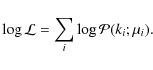
|
(1) |
In practice, we assign a low (non-zero) probability of having a star even in pixels where
To create the synthetic CMD, the program uses theoretical
isochrones either
from Padova (Marigo et al.
2008) or Geneva (Lejeune
& Schaerer 2001) or any other set of isochrones, as
long as they tabulate the relevant color versus mass. If the weight of
each isochrone were fitted independently, this would lead to a very
large
number of free parameters, due to the small difference in age between
individual isochrones, e.g.,
![]() for the Padova isochrones. We therefore group the isochrones together
in age bins that can be defined
by the user, typically using a bin size of
for the Padova isochrones. We therefore group the isochrones together
in age bins that can be defined
by the user, typically using a bin size of
![]() dex.
dex.
The program allows us to assign different weights to different rectangular regions of the CMD, selected by the user. This is useful because some phases of stellar evolution are more uncertain than others, e.g., the blue loop stars, and thus should carry less weight in the overall determination of the SFH. The use of completeness limits (if known) can be applied before the creation of the synthetic models, interpolating the completeness limits over the whole area of the CMD. The option of applying the completeness correction after the creation of the synthetic model is simply a multiplication of each pixel in the synthetic CMD with a number between 0 and 1. We also include a simplified treatment of binaries, in which binary evolution is ignored but the effect of unresolved binaries on the CMD are modeled. The program currently allows three different assumptions about the mass ratios in binary systems, namely a delta function, an IMF sampling and a flat distribution. The metallicity, (a range of) extinction values, and distance modulus must also be specified. We allow the extinction to be age-dependent, by providing a list of ages and a range of extinction values for each age. The program then interpolates in this list for each isochrone.
![\begin{figure}
\par\includegraphics[width=150mm,clip]{14267fg10.ps}
\end{figure}](/articles/aa/full_html/2010/08/aa14267-10/img89.png)
|
Figure 10:
SFH test using the bands B, V,
and I.
Artificial populations were created using Padova and Geneva isochrones
and then passed to the program. The procedure was performed
10 times and the mean SFH (dashed line) and the respective
standard deviation is shown, relative to the input assumed SFH of
|
| Open with DEXTER | |
Isochrones are populated by assuming a Salpeter
(1955) IMF with SFHs normalised to a mass range specify by
the user (
![]() is
the default range). Since we use Hess diagrams, each point in the
CMD is a density function. To construct them, different kernels, namely
square, Gaussian, disc, or delta function,
can be used. The kernels are of adjustable resolution and dimension. In
the test presented below, we adopted a resolution for the Hess diagrams
of
is
the default range). Since we use Hess diagrams, each point in the
CMD is a density function. To construct them, different kernels, namely
square, Gaussian, disc, or delta function,
can be used. The kernels are of adjustable resolution and dimension. In
the test presented below, we adopted a resolution for the Hess diagrams
of
![]() pixels
and used a delta function kernel. Each isochrone is broadened by the
assumed photometric errors and binarity, and shifted and broadened by
the (range of) specified extinction values.
To ensure a smooth coverage of the CMD, the program interpolates the
isochrones by
a factor of 10. After creating of the Hess diagram for each individual
isochrone, the program
linearly combines them and a synthetic CMD Hess diagram is obtained.
pixels
and used a delta function kernel. Each isochrone is broadened by the
assumed photometric errors and binarity, and shifted and broadened by
the (range of) specified extinction values.
To ensure a smooth coverage of the CMD, the program interpolates the
isochrones by
a factor of 10. After creating of the Hess diagram for each individual
isochrone, the program
linearly combines them and a synthetic CMD Hess diagram is obtained.
We performed a number of tests to check the internal consistency of the program, as well as the sensitivity of the derived SFHs to the various parameters involved.
5.2 Internal consistency check of the code
We created artificial stellar populations, passed them to the program,
and then checked how the output compared to the input. The populations
were constructed assuming a constant SFR of
![]() yr-1,
Padova or Geneva theoretical isochrones,
a Salpeter's IMF, and solar metallicity. The mass of each star was
randomly chosen using Salpeter's prescription for masses
between 1
and 100
yr-1,
Padova or Geneva theoretical isochrones,
a Salpeter's IMF, and solar metallicity. The mass of each star was
randomly chosen using Salpeter's prescription for masses
between 1
and 100 ![]() (low-mass stars (
(low-mass stars (![]() 1
1 ![]() )
are too faint to appear in the Hess diagram,
especially after applying a completeness limit). Because we restricted
the mass range
in our analysis, we then extrapolated to the default mass range used by
the code (
)
are too faint to appear in the Hess diagram,
especially after applying a completeness limit). Because we restricted
the mass range
in our analysis, we then extrapolated to the default mass range used by
the code (
![]() ).
The age of each star was assigned randomly (from a uniform
distribution) for ages between 4 Myr to 1 Gyr.
Having the mass and the age of each star, magnitudes were obtained by
interpolating the
theoretical isochrones. The magnitude limit used in these tests was MV
= 0.
We did not include binaries or extinction in this initial internal
consistency check of the code.
).
The age of each star was assigned randomly (from a uniform
distribution) for ages between 4 Myr to 1 Gyr.
Having the mass and the age of each star, magnitudes were obtained by
interpolating the
theoretical isochrones. The magnitude limit used in these tests was MV
= 0.
We did not include binaries or extinction in this initial internal
consistency check of the code.
Figure 10 presents the results of this analysis. In all the panels, the input SFH is shown as a horizontal straight line and the average reconstructed SFH of the output after 10 different runs as dashed lines. Each run had a new population, i.e., different random realization, for the bands B, V, and I. The error bars illustrate the standard deviation in the reconstructed SFHs. We studied the variations in these results based on the different assumptions of binning. Three different bins were used in this test corresponding to each row of Fig. 10.
We see that the reconstructed star formation histories
generally agree
fairly
well with the input values regardless of the binning, color, or
isochrones used. It is observed that the error bars are larger for
smaller bins, although good agreement with the input SFH is
maintained. The maximum difference is
![]() dex,
and generally far less.
dex,
and generally far less.
We performed a test to see how completeness affects our SFH estimation. Figure 11 shows the Hess diagram of a stellar population with ages between 106 to 109 yr using the mass range from above. Overplotted are 3 Padova 2008 isochrones for ages 107, 108, and 109 yr and four completeness limits at MV = -0.5,0.0,0.5, and 1.0 mag. Figure 12 shows that the SFHs can be recovered reliably to progressively older ages as the completeness limit becomes fainter. In particular, the ``burst'' at 108.8 years disappears when fainter stars are included in the fit.
Cignoni & Tosi (2010) created artificial CMDs to simulate a stellar population with a constant SFR between 0-13 Gyr and used four different completeness limits. They concluded that to safely reconstruct a SFH over a full Hubble time from a CMD, we need to resolve all stars down to MV=4.5. However, this completeness limit can only be reached for galaxies in the Local Group.
We conclude that our program produces consistent results at the level of 0.05 dex, the age range over which this holds being restricted mainly by the completeness limits. This internal consistency of the code does not, however, imply that real SFHs can be recovered with similar accuracy.
5.3 Tests of sensitivity to assumptions about parameters
We now concentrate on testing the effects of four parameters:
metallicity, extinction, binarity, and the fitting area used
(rectangular boxes). To perform this test, we executed the code using
the scientific data described in Sect. 4, using different
assumptions
about these parameters and a mass range
![]() (which is the same mass range used in Sect. 5.4). The results
are shown in
Fig. 13.
Each panel represents one of the tested variables.
(which is the same mass range used in Sect. 5.4). The results
are shown in
Fig. 13.
Each panel represents one of the tested variables.
In panel a), we show the SFHs derived for
three assumptions about
metallicity: solar (Z=0.02), LMC (Z=0.008),
and SMC (Z=0.004).
In this panel, we ignore binaries, include no additional extinction and
used the fitting area called ``boxes2'' described below. We observed
that the SFH
does not change very much from LMC to solar, but at SMC metallicity
there is a much stronger increase from ![]() 100 Myr
ago to the present. By comparing the observed and model Hess diagrams,
it is clear that the solar metallicity isochrones
generally provide a poor fit, especially for the red and blue
supergiants that
appear much too cool compared to the observations, while LMC and SMC
metallicities are very similar (see Fig. 14).
100 Myr
ago to the present. By comparing the observed and model Hess diagrams,
it is clear that the solar metallicity isochrones
generally provide a poor fit, especially for the red and blue
supergiants that
appear much too cool compared to the observations, while LMC and SMC
metallicities are very similar (see Fig. 14).
Panel b) presents the behavior of the SFHs for three different assumptions about the total extinction (foreground plus internal): Ab=[0.1,0.15,0.2]. We fixed the metallicity at Z=0.008 (LMC), again ignoring binaries, used Padova isochrones and used the fitting area ``boxes2''. In general, the SFHs obtained using different extinctions do not vary strongly for these relatively modest variations in the extinction. Greater extinction variations would produce larger shifts towards the red in the model Hess diagrams and are inconsistent with the data.
Panel c) shows the dependence on the
assumptions for binary fraction (f) and mass ratio (q)
of values (1.) f=0, q=0; (2.) f=0.5,
q=[0.1,0.9];
(3.) f=1, q=1. The panel also
indicates how this dependence affects the estimation of the SFHs. We
used Padova isochrones, fixed the metallicity at Z=0.008,
ignored
the effects of additional extinction, and used the fitting area named
"boxes2" described below. Binarity can have an effect on the derived
SFHs with minor effects for ![]() Myr
and a shift towards somewhat lower overall SFR for the extreme case f
and q equal 1.
However, the binarity assumptions made here are not completely
realistic. The first and third assumptions are extreme cases with no
binaries at all and a galaxy where
all the stars have a companion of exactly the same mass, respectively.
The second assumption is an intermediate case where there is a
continuous (flat) range of q values and a
star has
Myr
and a shift towards somewhat lower overall SFR for the extreme case f
and q equal 1.
However, the binarity assumptions made here are not completely
realistic. The first and third assumptions are extreme cases with no
binaries at all and a galaxy where
all the stars have a companion of exactly the same mass, respectively.
The second assumption is an intermediate case where there is a
continuous (flat) range of q values and a
star has ![]() 50%
probability of being in a binary system. However, in a more
realistic case binary evolution should be taken
into account as well. This is however beyond the scope of the present
work.
50%
probability of being in a binary system. However, in a more
realistic case binary evolution should be taken
into account as well. This is however beyond the scope of the present
work.
![\begin{figure}
\par\includegraphics[width=9cm,clip]{14267fg11.ps}
\end{figure}](/articles/aa/full_html/2010/08/aa14267-10/img96.png)
|
Figure 11: Hess diagram for the 4 possible completeness limit studied in Fig. 12. |
| Open with DEXTER | |
![\begin{figure}
\par\includegraphics[width=9cm,clip]{14267fg12.ps}
\end{figure}](/articles/aa/full_html/2010/08/aa14267-10/img97.png)
|
Figure 12: Test of the SFH using different completeness limits. |
| Open with DEXTER | |
In the last panel, panel d), we show the SFH
estimates obtained using two different sets of boxes in the fitting.
As overplotted in Fig. 17, where
we plot the observed Hess diagram and the regions fitted, the left box
(
![]() and
and
![]() )
used contains the main sequence stars, the blue He core burning phases
being outside of the fit, while the right box (
)
used contains the main sequence stars, the blue He core burning phases
being outside of the fit, while the right box (
![]() and
and
![]() )
contains the red He core burning stars and possible RGBs and AGBs. This
set of boxes is called ``boxes2''. The second set of boxes covers the
same area for the evolved stars (right box), while
the blue He core burning stars are also included in the fitting box (
)
contains the red He core burning stars and possible RGBs and AGBs. This
set of boxes is called ``boxes2''. The second set of boxes covers the
same area for the evolved stars (right box), while
the blue He core burning stars are also included in the fitting box (
![]() ),
which we label ``boxes1'' in panel d). In general,
we found that, the SFH result from "boxes2" shows a lower value that
for ``boxes1''. We
studied these two possible sets of boxes because the fitted Hess
diagrams retrieved using these two boxes
indicated that the fit for the blue He core burning stars is not in
good agreement with observations. The variations after
),
which we label ``boxes1'' in panel d). In general,
we found that, the SFH result from "boxes2" shows a lower value that
for ``boxes1''. We
studied these two possible sets of boxes because the fitted Hess
diagrams retrieved using these two boxes
indicated that the fit for the blue He core burning stars is not in
good agreement with observations. The variations after ![]()
![]() 108.7 yr
are unlikely to be real, but are probably due to incompleteness as
discussed above.
108.7 yr
are unlikely to be real, but are probably due to incompleteness as
discussed above.
We created a fake population using Padova isochrones and
assuming solar metallicity, no extinction, and no binarity; we then
analyze this with our program, using Geneva isochrones to see whether
the assumed SFH could be recovered. Figure 16 shows the
result of this test. There are significant differences between the
input and recovered SFH, deviations being as large as ![]() 0.4 dex
at young ages (<10 Myr) and differences being at the
level of 0.1-0.2 dex at older ages.
The error bars presented in Fig. 16
were determined using the same method used in the previous section,
i.e., are equivalent to the standard deviation of the reconstructed
SFHs after 10 different runs with different random
realizations.
0.4 dex
at young ages (<10 Myr) and differences being at the
level of 0.1-0.2 dex at older ages.
The error bars presented in Fig. 16
were determined using the same method used in the previous section,
i.e., are equivalent to the standard deviation of the reconstructed
SFHs after 10 different runs with different random
realizations.
We finally test how random errors (due to the finite number of stars in the Hess diagram) affect the SFHs, using a bootstrapping method whereby the input data, i.e., the photometric data found in this work, are randomly resampled many times. To perform this test, we used the observations obtained in this work (see Sect. 4), Padova 2008 isochrones, LMC metallicity, no additional extinction, and no binarity. Disabling binarity will not influence our results dramatically and will save us computational time. We ran the program 100 times, redistributing randomly the photometric data in each run. From Fig. 15, we conclude that Poisson variations do not significantly affect our results.
To summarize, we demonstrated that the main uncertainties in our derived SFHs are systematic, depending on assumptions about binarity, the choice of isochrones, and metallicity. However, with the exception of the use of solar metallicity isochrones (which provide a poor fit to the data), the overall mean SFRs are fairly consistent with our data up to ages of a few hundred Myr.
5.4 Results
To infer the SFH of NGC 4395, we combined both fields
to be
able to directly compare with the cluster age distribution. The
differences in our completeness limits for each band and each field are
smaller than 0.1 mag,
allowing us to use the completeness values obtained in our first field
(results for the second field can also be used instead) to study the
SFH of the whole galaxy. In the SFH reconstruction, we used a
resolution of ![]() pixels
for the Hess diagrams and a Gaussian kernel with a standard deviation
of 0.02 mag in V-I(or B-V).
Based on our observed Hess diagram we used 2 rectangular fitting areas (boxes2)
for the SFH reconstruction
with the same limits as described in the previous section. To check the
consistency of our results we performed the analysis using both
B-V and V-I
colors, using the same parameters and boxes to fit the data.
pixels
for the Hess diagrams and a Gaussian kernel with a standard deviation
of 0.02 mag in V-I(or B-V).
Based on our observed Hess diagram we used 2 rectangular fitting areas (boxes2)
for the SFH reconstruction
with the same limits as described in the previous section. To check the
consistency of our results we performed the analysis using both
B-V and V-I
colors, using the same parameters and boxes to fit the data.
Figure 17
depicts the observed (left) and best-fit model (right) Hess diagrams
(assuming f=0.5 and
q=[0.1,0.9]).
The final combination of parameters used to estimate the SFH
were Padova 2008 isochrones, a Salpeter IMF (M=[0.10,100] ![]() ), LMC
metallicity, three different assumptions for the binarity, distance
modulus of 28.1, a total extinction of AB=0.15,
and the photometric errors and completeness limit obtained in
Sect. 4.
), LMC
metallicity, three different assumptions for the binarity, distance
modulus of 28.1, a total extinction of AB=0.15,
and the photometric errors and completeness limit obtained in
Sect. 4.
![\begin{figure}
\par\includegraphics[width=15.6cm,clip]{14267fg13.ps}
\vspace*{6mm}
\end{figure}](/articles/aa/full_html/2010/08/aa14267-10/img105.png)
|
Figure 13: Padova theoretical isochrones were used to test the SFH program developed using the photometric data obtained in Sect. 4. Panel a): test for different metallicities (solar, LMC, SMC) without binarity or extinction assumed. Panel b): test for different extinctions assuming LMC metallicity and no binarity. Panel c): test for different binarity assuming LMC metallicity and no extinction. Panel d): test for different boxes used over the fitting data assuming LMC metallicity, no extinction, and no binarity. |
| Open with DEXTER | |
![\begin{figure}
\par\includegraphics[width=9cm,clip]{14267fg14.ps}
\end{figure}](/articles/aa/full_html/2010/08/aa14267-10/img106.png)
|
Figure 14: Comparison of the fit for different metallicities (solar, LMC, and SMC). |
| Open with DEXTER | |
![\begin{figure}
\par\includegraphics[width=9cm,clip]{14267fg15.ps}
\end{figure}](/articles/aa/full_html/2010/08/aa14267-10/img107.png)
|
Figure 15: Bootstrapping study. The errors retrieved from this test are the random errors of our program. No strong variations caused by random errors affect our results. |
| Open with DEXTER | |
![\begin{figure}
\par\includegraphics[width=9cm,clip]{14267fg16.ps}
\end{figure}](/articles/aa/full_html/2010/08/aa14267-10/img108.png)
|
Figure 16: Test using Padova isochrones to create the population and Geneva isochrones to analyze them. |
| Open with DEXTER | |
![\begin{figure}
\par\includegraphics[width=9cm,clip]{14267fg17.ps}
\end{figure}](/articles/aa/full_html/2010/08/aa14267-10/img109.png)
|
Figure 17:
Comparison between the observed and fitted Hess diagrams for the field
stars studied in this work. As age indicators, three isochrones are
overplotted at the ages of
|
| Open with DEXTER | |
![\begin{figure}
\par\includegraphics[width=9cm,clip]{14267fg18.ps}
\end{figure}](/articles/aa/full_html/2010/08/aa14267-10/img110.png)
|
Figure 18: SFH for the galaxy NGC 4395. We studied the SFH for three different assumptions about the binaries trying to cover possible combinations between binary fraction and mass ratio for the colors V-I ( left panel) and B-V ( right panel). |
| Open with DEXTER | |
The phases that are most accurately reproduced by the fit are the main sequence, red core-He burning, and RGB/AGB phases. For the blue core-He burning phases, the model fit is less good, being redder than observed and with a more pronounced gap between the main sequence and blue core-He burning stars in the model than in the data. This is a generic problem with the isochrones that exists for any star formation history we adopt.
Our most accurate estimates of the extinction were obtained by
trial and error. We compared the main sequence stars from
the fitted Hess diagram with data for those observed and assumed
different values (
AB=[0.1,0.15,0.2])
for the total extinction
until we obtained the best fit between the two Hess diagrams
(considering the main sequence only). The difference between the
foreground value (
AB
= 0.074) and our best-fit model value (
![]() )
suggests a low internal extinction in NGC 4395 of
)
suggests a low internal extinction in NGC 4395 of
![]() mag.
This estimation was performed for LMC metallicity.
mag.
This estimation was performed for LMC metallicity.
The estimated SFHs (for V-I
and B-V) are shown in
Fig. 18.
As discussed in the previous section, the SFHs become very uncertain at
ages greater than a few hundred Myr; the apparent burst at ![]() 108.4 yr
is probably not real. There is also a hint of a rapid drop at very
young ages in V-I (
108.4 yr
is probably not real. There is also a hint of a rapid drop at very
young ages in V-I (![]() 106.8 years),
but this may be caused by
uncertainties in the isochrones. Furthermore, the youngest age included
in our artificial Hess diagrams is 4 Myr; if younger stars
were
present in the field, these would be included in the youngest bin. The
appropriate lower age limit depends on how long young stars
are embedded in their native molecular clouds. We present the SFHs for
different binarity assumptions because this parameter is also
uncertain. We use the same 3 choices in Fig. 18 as those
used in Fig. 13
above. Taking the values for each bin (in linear units), we estimated
the average star formation rate for ages between 107
and 108 years using the colors V-I
and B-V, as shown in Table 3.
106.8 years),
but this may be caused by
uncertainties in the isochrones. Furthermore, the youngest age included
in our artificial Hess diagrams is 4 Myr; if younger stars
were
present in the field, these would be included in the youngest bin. The
appropriate lower age limit depends on how long young stars
are embedded in their native molecular clouds. We present the SFHs for
different binarity assumptions because this parameter is also
uncertain. We use the same 3 choices in Fig. 18 as those
used in Fig. 13
above. Taking the values for each bin (in linear units), we estimated
the average star formation rate for ages between 107
and 108 years using the colors V-I
and B-V, as shown in Table 3.
There is an apparent increase in the SFR between
![]() and
and ![]() ,
of
,
of ![]() 0.5 dex.
Based in Fig. 18,
the average star formation rate over the past 108 years
is
0.5 dex.
Based in Fig. 18,
the average star formation rate over the past 108 years
is ![]() yr-1within
the two ACS fields (assuming f=0.5 and
q=[0.1,0.9]).
We note that this is a factor of 4 higher than the global
SFR for
NGC 4395 that follows from using the far-infrared luminosity
described in Larsen & Richtler
(2000), who
used the calibration by Buat
& Xu (1996). This highlights the difficulty in
determining extragalactic star formation rates from integrated light.
yr-1within
the two ACS fields (assuming f=0.5 and
q=[0.1,0.9]).
We note that this is a factor of 4 higher than the global
SFR for
NGC 4395 that follows from using the far-infrared luminosity
described in Larsen & Richtler
(2000), who
used the calibration by Buat
& Xu (1996). This highlights the difficulty in
determining extragalactic star formation rates from integrated light.
5.5 Ages and masses of clusters
After identifying the star cluster candidates (see Sect. 4) in the two
fields,
we need to estimate their masses and ages. These parameters were
estimated using the program AnalySED, created by
Anders et al. (2004).
This program determines the masses and ages
using GALEV SSP evolutionary models (Schulz
et al. 2002). The parameters used for AnalySED are a
Salpeter IMF (Salpeter 1955)
in the mass range 0.10 to 100 ![]() ,
Padova isochrones (Girardi
et al. 2000), and a LMC metallicity.
AnalySED performs a match, comparing the observed and
theoretical spectral energy distributions (SEDs), based on GALEV SSP
models. As
output, AnalySED provides, among other parameters, an estimation of the
mass and the age for each cluster.
,
Padova isochrones (Girardi
et al. 2000), and a LMC metallicity.
AnalySED performs a match, comparing the observed and
theoretical spectral energy distributions (SEDs), based on GALEV SSP
models. As
output, AnalySED provides, among other parameters, an estimation of the
mass and the age for each cluster.
In addition to our magnitude limit of V=23
(![]() )
for our clusters, we also define a lower mass
limit at
)
for our clusters, we also define a lower mass
limit at ![]() to increase the likelihood that extended objects are true clusters and
not just chance projections of a few bright stars. However, over most
of the age range (
to increase the likelihood that extended objects are true clusters and
not just chance projections of a few bright stars. However, over most
of the age range (
![]() ),
these false detections would fall below our magnitude limit.
),
these false detections would fall below our magnitude limit.
Table 3:
Average star formation rate [in ![]() Yr-1]
over the past 108 years, estimated
using different binarity, colors, and isochrones.
Yr-1]
over the past 108 years, estimated
using different binarity, colors, and isochrones.
Figure 19
shows the
age-mass diagram of the cluster candidates in NGC 4395. The
number
of clusters detected is rather small because the two HST pointings do
not cover the whole galaxy and our coverage for clusters is reduced
further by our requirement of the WFPC2 pointings for
age-dating.
We see that neither massive (
![]() )
nor old (
)
nor old (
![]() yr) clusters
are detected, in agreement with previous work (Mora et al. 2009; Larsen &
Richtler 1999). We identified few clusters with
yr) clusters
are detected, in agreement with previous work (Mora et al. 2009; Larsen &
Richtler 1999). We identified few clusters with ![]() Myr
for LMC metallicity in agreement with Mora
et al. (2009),
although the number of objects was greater in their work. Nevertheless,
the number of objects detected at these ages (and greater) varies, as
can be see in Fig. 7
of Mora et al., depending on the metallicity used to estimate
the parameters.
Myr
for LMC metallicity in agreement with Mora
et al. (2009),
although the number of objects was greater in their work. Nevertheless,
the number of objects detected at these ages (and greater) varies, as
can be see in Fig. 7
of Mora et al., depending on the metallicity used to estimate
the parameters.
![\begin{figure}
\par\includegraphics[width=9cm,clip]{14267fg19.ps}
\end{figure}](/articles/aa/full_html/2010/08/aa14267-10/img121.png)
|
Figure 19: Age-mass distribution of the clusters detected in our two fields observed. The red dashed line represents MV=-5. Symbols are the same as in Fig. 6. |
| Open with DEXTER | |
6 Summary, discussion, and conclusions
We have described our procedures to obtain the age distributions
of field stars and star clusters in HST images of nearby (![]() Mpc)
galaxies, in particular, we have described our implementation of the
synthetic CMD method and tests of our program developed for this
purpose. We found that the code recovers the star formation histories
of synthetic
populations with good accuracy, while errors in the derived SFHs
of true populations are dominated by systematics errors. We have
derived the SFH for NGC 4395 for three different metallicities
and find an approximately constant SFR over the past few
hundred Myr
assuming LMC-like metallicity. Only a modest amount of internal
extinction (
Mpc)
galaxies, in particular, we have described our implementation of the
synthetic CMD method and tests of our program developed for this
purpose. We found that the code recovers the star formation histories
of synthetic
populations with good accuracy, while errors in the derived SFHs
of true populations are dominated by systematics errors. We have
derived the SFH for NGC 4395 for three different metallicities
and find an approximately constant SFR over the past few
hundred Myr
assuming LMC-like metallicity. Only a modest amount of internal
extinction (
![]() )
in NGC 4395 is required in addition to the Galactic foreground
extinction to match the data. Hence, uncertainties in the total
extinction
is not a major source of error compared to, for example, binary stars
and the choice of isochrones. Different assumptions may lead to changes
in our estimated SFRs of up to a factor of 2-4 in specific age bins,
although the global average will be less affected. Poissonian errors do
not contribute substantially to the uncertainties because of the large
number of field stars used in our analysis.
)
in NGC 4395 is required in addition to the Galactic foreground
extinction to match the data. Hence, uncertainties in the total
extinction
is not a major source of error compared to, for example, binary stars
and the choice of isochrones. Different assumptions may lead to changes
in our estimated SFRs of up to a factor of 2-4 in specific age bins,
although the global average will be less affected. Poissonian errors do
not contribute substantially to the uncertainties because of the large
number of field stars used in our analysis.
After estimating the SFH of the field stars and both the age and mass distributions of star clusters, we can now measure which fraction of stars are in clusters. We compare the fractions for cluster ages between 107 and 108 years, since disruption due to tidal shocks (GMC and spiral arm encounters) and evaporation is expected to become significant at older ages, while younger objects may still be unbound and prone to ``infant mortality''.
A rough estimate of the cluster formation rate (CFR) can be
obtained by dividing the total amount of mass in clusters observed by
the age range. From ![]() yr,
the total mass observed in Fig. 19 is
yr,
the total mass observed in Fig. 19 is
![]() ,
which
infers a
,
which
infers a ![]() [
[![]() yr-1].
We correct this for the smaller area covered by the WFPC2 camera
compared to the ACS (a factor of
yr-1].
We correct this for the smaller area covered by the WFPC2 camera
compared to the ACS (a factor of ![]() 2.27) and thus obtain
2.27) and thus obtain
![]() [
[![]() yr-1]
for the same equivalent area covered by our field star data.
yr-1]
for the same equivalent area covered by our field star data.
A magnitude-limited sample does not allow us to observe all
the clusters in the age range. Using the observed total mass and
assuming a cluster
mass function (![]() ),
we can estimate the total mass in clusters for a certain age range. Larsen (2009) showed that a
Schechter function (with
),
we can estimate the total mass in clusters for a certain age range. Larsen (2009) showed that a
Schechter function (with
![]() )
can model the initial cluster mass function in present-day spiral
discs. However, the canonical cluster mass function, a power law with
index -2, can be used for the same purpose. To estimate the
cluster formation rate we used both functions and calculated
the total mass in the age range mentioned above. Since the most massive
clusters observed have
)
can model the initial cluster mass function in present-day spiral
discs. However, the canonical cluster mass function, a power law with
index -2, can be used for the same purpose. To estimate the
cluster formation rate we used both functions and calculated
the total mass in the age range mentioned above. Since the most massive
clusters observed have ![]() ,
it makes little difference whether we adopt the Schechter function or
an untruncated power-law.
,
it makes little difference whether we adopt the Schechter function or
an untruncated power-law.
The total mass in the cluster system was estimated using the
equation
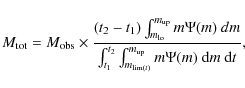
where t1,t2 represent the time interval ( t1 = 107 years, t2 = 108 years),
![\begin{figure}
\par\includegraphics[width=9cm,clip]{14267fg20.ps}
\end{figure}](/articles/aa/full_html/2010/08/aa14267-10/img142.png)
|
Figure 20:
Relation between the cluster formation efficiency ( |
| Open with DEXTER | |
Our estimate of ![]() is lower than the value
is lower than the value
![]() obtained by
Bastian (2008). Gieles (2009) estimated
obtained by
Bastian (2008). Gieles (2009) estimated ![]() for three galaxies namely M 74, M 101, and
M 51. The
cluster formation rate was estimated by comparing theoretical with
empirical luminosity functions. Gieles suggested that
for three galaxies namely M 74, M 101, and
M 51. The
cluster formation rate was estimated by comparing theoretical with
empirical luminosity functions. Gieles suggested that ![]() has the tendency to increase with SFR. Gieles & Bastian (2008)
estimated
has the tendency to increase with SFR. Gieles & Bastian (2008)
estimated
![]() for the SMC using an accurate
determination of the mean global star
formation rate based on the field stars (SFR
for the SMC using an accurate
determination of the mean global star
formation rate based on the field stars (SFR
![]() yr-1)
performed by Harris &
Zaritsky (2004) and the CFR calculated in their work. Other
studies have found the same value for
yr-1)
performed by Harris &
Zaritsky (2004) and the CFR calculated in their work. Other
studies have found the same value for ![]() in the SMC (see Goddard
et al. 2010). We took the data from Gieles (2009) (see Table 1 in his article),
and Gieles & Bastian
(2008)
and plotted the total formation rate (
in the SMC (see Goddard
et al. 2010). We took the data from Gieles (2009) (see Table 1 in his article),
and Gieles & Bastian
(2008)
and plotted the total formation rate (
![]() )
against
)
against ![]() for these four galaxies and included our CFR and SFR for
NGC 4395 to attempt to detect any correlation. Figure 20 shows the
plot of
for these four galaxies and included our CFR and SFR for
NGC 4395 to attempt to detect any correlation. Figure 20 shows the
plot of ![]() versus
versus ![]() .
There is an apparent
correlation between these two values, which can be approximated by a
power law
.
There is an apparent
correlation between these two values, which can be approximated by a
power law
![]() .
Although only five points are plotted and the TFR in NGC 4395
does not cover the whole galaxy, Fig. 20 does
suggest that the relatively low
.
Although only five points are plotted and the TFR in NGC 4395
does not cover the whole galaxy, Fig. 20 does
suggest that the relatively low ![]() value we derive for NGC 4395 is consistent with a general
trend. In a future study (Silva-Villa et al. 2010, in prep.),
we will include
more points in this plot for galaxies spanning a range in TFR and check
the validity of this result.
value we derive for NGC 4395 is consistent with a general
trend. In a future study (Silva-Villa et al. 2010, in prep.),
we will include
more points in this plot for galaxies spanning a range in TFR and check
the validity of this result.
Goddard et al.
(2010) found an empirical relation between ![]() and the SFR density (
and the SFR density (
![]() [
[![]() yr-1 Kpc-2]).
We estimated
yr-1 Kpc-2]).
We estimated ![]() to be
to be ![]()
![]() yr-1 Kpc-2
for NGC 4395, which leads to
yr-1 Kpc-2
for NGC 4395, which leads to
![]() based
on the
Goddard et al. (2010)
relation. This value is higher than
that estimated in this work
based
on the
Goddard et al. (2010)
relation. This value is higher than
that estimated in this work
![]() .
We point out that the area covered by our observations is not the total
area of the galaxy and so the SFR
density found in this work might be higher than the global average.
.
We point out that the area covered by our observations is not the total
area of the galaxy and so the SFR
density found in this work might be higher than the global average.
Silva-Villa would like to thank Peter Anders for help with the program AnalySED. We thank C. U. Keller and the referee for comments that helped improve this article.
References
- Anders, P., & Fritze-v. Alvensleben, U. 2003, A&A, 401, 1063 [NASA ADS] [CrossRef] [EDP Sciences] [Google Scholar]
- Anders, P., Bissantz, N., Fritze-v. Alvensleben, U., et al. 2004, MNRAS, 347, 196 [NASA ADS] [CrossRef] [Google Scholar]
- Annibali, F., Tosi, M., Monelli, M., et al. 2009, AJ, 138, 169 [NASA ADS] [CrossRef] [Google Scholar]
- Aparicio, A., & Gallart, C. 2004, AJ, 128, 1465 [NASA ADS] [CrossRef] [Google Scholar]
- Aparicio, A., & Hidalgo, S. L. 2009, AJ, 138, 558 [NASA ADS] [CrossRef] [MathSciNet] [Google Scholar]
- Aparicio, A., Gallart, C., & Bertelli, G. 1997, AJ, 114, 669 [NASA ADS] [CrossRef] [Google Scholar]
- Barker, M. K., Sarajedini, A., Geisler, D., Harding, P., & Schommer, R. 2007, AJ, 133, 1138 [Google Scholar]
- Bastian, N. 2008, MNRAS, 390, 759 [NASA ADS] [CrossRef] [Google Scholar]
- Bastian, N., & Gieles, M. 2008, in Mass Loss from Stars and the Evolution of Stellar Clusters, ed. A. de Koter, L. J. Smith, & L. B. F. M. Waters, ASP Conf. Ser., 388, 353 [Google Scholar]
- Baumgardt, H. 2009, Dissolution of Globular Clusters, ed. T. Richtler, & S. Larsen, 387 [Google Scholar]
- Bertelli, G., Bressan, A., Chiosi, C., Fagotto, F., & Nasi, E. 1994, A&AS, 106, 275 [NASA ADS] [Google Scholar]
- Bertin, E., & Arnouts, S. 1996, A&AS, 117, 393 [NASA ADS] [CrossRef] [EDP Sciences] [Google Scholar]
- Boutloukos, S. G., & Lamers, H. J. G. L. M. 2003, MNRAS, 338, 717 [NASA ADS] [CrossRef] [Google Scholar]
- Brown, T. M., Beaton, R., Chiba, M., et al. 2008, ApJ, 685, L121 [NASA ADS] [CrossRef] [Google Scholar]
- Buat, V., & Xu, C. 1996, A&A, 306, 61 [NASA ADS] [Google Scholar]
- Cerviño, M., & Luridiana, V. 2006, A&A, 451, 475 [NASA ADS] [CrossRef] [EDP Sciences] [Google Scholar]
- Cignoni, M., & Tosi, M. 2010, Advances in Astronomy, 2010, 3 [Google Scholar]
- Cole, A. A., Skillman, E. D., Tolstoy, E., et al. 2007, ApJ, 659, L17 [NASA ADS] [CrossRef] [Google Scholar]
- Dolphin, A. 1997, New Astron., 2, 397 [NASA ADS] [CrossRef] [Google Scholar]
- Dolphin, A. E. 2000, PASP, 112, 1397 [NASA ADS] [CrossRef] [Google Scholar]
- Edvardsson, B., Andersen, J., Gustafsson, B., et al. 1993, A&A, 275, 101 [NASA ADS] [Google Scholar]
- Elmegreen, B. G. 2008, 388, 249 [Google Scholar]
- Fall, S. M. 2006, ApJ, 652, 1129 [NASA ADS] [CrossRef] [Google Scholar]
- Filippenko, A. V., & Sargent, W. L. W. 1989, ApJ, 342, L11 [NASA ADS] [CrossRef] [Google Scholar]
- Forbes, D. A., Brodie, J. P., & Huchra, J. 1997, AJ, 113, 887 [NASA ADS] [CrossRef] [Google Scholar]
- Gieles, M. 2009, [arXiv:0908.2974] [Google Scholar]
- Gieles, M., & Bastian, N. 2008, A&A, 482, 165 [NASA ADS] [CrossRef] [EDP Sciences] [Google Scholar]
- Girardi, L., Bressan, A., Bertelli, G., et al. 2000, A&AS, 141, 371 [Google Scholar]
- Girardi, L., Chiosi, C., Bertelli, G., et al. 1995, A&A, 298, 87 [NASA ADS] [Google Scholar]
- Goddard, Q. E., Bastian, N., & Kennicutt, R. C. 2010, MNRAS, 405, 857 [NASA ADS] [Google Scholar]
- Grevesse, N., & Sauval, A. J. 1998, Space Sci. Rev., 85, 161 [NASA ADS] [CrossRef] [Google Scholar]
- Harris, J., & Zaritsky, D. 2001, ApJS, 136, 25 [NASA ADS] [CrossRef] [Google Scholar]
- Harris, J., & Zaritsky, D. 2002, in Observed HR Diagrams and Stellar Evolution, ed. T. Lejeune & J. Fernandes, ASP Conf. Ser., 274, 600 [Google Scholar]
- Harris, J., & Zaritsky, D. 2004, AJ, 127, 1531 [NASA ADS] [CrossRef] [Google Scholar]
- Harris, J., & Zaritsky, D. 2009, AJ, 138, 1243 [NASA ADS] [CrossRef] [Google Scholar]
- King, I. 1962, AJ, 67, 471 [NASA ADS] [CrossRef] [Google Scholar]
- Koekemoer, A. M., Fruchter, A. S., Hook, R. N., et al. 2002, in The 2002 HST Calibration Workshop : Hubble after the Installation of the ACS and the NICMOS Cooling System, ed. S. Arribas, A. Koekemoer, & B. Whitmore, 337 [Google Scholar]
- Lada, C. J., & Lada, E. A. 2003, ARA&A, 41, 57 [NASA ADS] [CrossRef] [Google Scholar]
- Lamers, H. J. G. L. M., & Gieles, M. 2008, in Mass Loss from Stars and the Evolution of Stellar Clusters, ed. A. de Koter, L. J. Smith, & L. B. F. M. Waters, ASP Conf. Ser., 388, 367 [Google Scholar]
- Lamers, H. J. G. L. M., Gieles, M., Bastian, N., et al. 2005, A&A, 441, 117 [NASA ADS] [CrossRef] [EDP Sciences] [Google Scholar]
- Larsen, S. S. 1999, A&AS, 139, 393 [NASA ADS] [CrossRef] [EDP Sciences] [Google Scholar]
- Larsen, S. S. 2009, A&A, 503, 467 [NASA ADS] [CrossRef] [EDP Sciences] [Google Scholar]
- Larsen, S. S., & Richtler, T. 1999, A&A, 345, 59 [NASA ADS] [Google Scholar]
- Larsen, S. S., & Richtler, T. 2000, A&A, 354, 836 [NASA ADS] [Google Scholar]
- Larsen, S. S., Forbes, D. A., & Brodie, J. P. 2001, MNRAS, 327, 1116 [NASA ADS] [CrossRef] [Google Scholar]
- Larsen, S. S., Efremov, Y. N., Elmegreen, B. G., et al. 2002, ApJ, 567, 896 [NASA ADS] [CrossRef] [Google Scholar]
- Larsen, S. S., Mora, M. D., Brodie, J. P., & Richtler, T 2007, in IAU Symp. 241, ed. A. Vazdekis & R. F. Peletier, 435 [Google Scholar]
- Lejeune, T., & Schaerer, D. 2001, A&A, 366, 538 [NASA ADS] [CrossRef] [EDP Sciences] [Google Scholar]
- Maíz Apellániz, J. 2009, ApJ, 699, 1938 [NASA ADS] [CrossRef] [Google Scholar]
- Marigo, P., Girardi, L., Bressan, A., et al. 2008, A&A, 482, 883 [NASA ADS] [CrossRef] [EDP Sciences] [Google Scholar]
- Mateo, M. L. 1998, ARA&A, 36, 435 [NASA ADS] [CrossRef] [Google Scholar]
- Mora, M. D., Larsen, S. S., & Kissler-Patig, M. 2007, A&A, 464, 495 [NASA ADS] [CrossRef] [EDP Sciences] [Google Scholar]
- Mora, M. D., Larsen, S. S., Kissler-Patig, M., Brodie, J. P., & Richtler, T. 2009, A&A, 501, 949 [NASA ADS] [CrossRef] [EDP Sciences] [Google Scholar]
- Rejkuba, M., Greggio, L., & Zoccali, M. 2004, A&A, 415, 915 [NASA ADS] [CrossRef] [EDP Sciences] [Google Scholar]
- Roy, J., Belley, J., Dutil, Y., et al. 1996, ApJ, 460, 284 [NASA ADS] [CrossRef] [Google Scholar]
- Salpeter, E. E. 1955, ApJ, 121, 161 [Google Scholar]
- Schlegel, D. J., Finkbeiner, D. P., & Davis, M. 1998, ApJ, 500, 525 [NASA ADS] [CrossRef] [Google Scholar]
- Schulz, J., Fritze-v. Alvensleben, U., Möller, C. S., et al. 2002, A&A, 392, 1 [NASA ADS] [CrossRef] [EDP Sciences] [Google Scholar]
- Sirianni, M., Jee, M. J., Benítez, N., et al. 2005, PASP, 117, 1049 [NASA ADS] [CrossRef] [Google Scholar]
- Skillman, E. D., & Gallart, C. 2002, in Observed HR Diagrams and Stellar Evolution, ed. T. Lejeune & J. Fernandes, ASP Conf. Ser., 274, 535 [Google Scholar]
- Spitzer, L. 1987, Dynamical evolution of globular clusters, ed. L. Spitzer [Google Scholar]
- Tosi, M., Greggio, L., Marconi, G., et al. 1991, AJ, 102, 951 [NASA ADS] [CrossRef] [Google Scholar]
- Whitmore, B. C. 2007, in IAU Symposium, ed. B. G. Elmegreen & J. Palous, IAU Symposium, 237, 222 [Google Scholar]
- Williams, B. F., Dalcanton, J. J., Seth, A. C., et al. 2009, AJ, 137, 419 [NASA ADS] [CrossRef] [Google Scholar]
- Young, L. M., Skillman, E. D., Weisz, D. R., et al. 2007, ApJ, 659, 331 [NASA ADS] [CrossRef] [Google Scholar]
Footnotes
- ... IRAF
![[*]](/icons/foot_motif.png)
- IRAF is distributed by the National Optical Astronomical Observatory (NOAO), which is operated by the Association of Universities for Research in Astronomy, Inc, under cooperative agreement with the National Science Foundation
- ... webpages
- http://www.stsci.edu/hst/acs/analysis/zeropoints/#tablestart
- ... webpages
- www.stsci.edu/instruments/wfpc2/Wfpc2_ch52#1933986
- ...Dolphin (2000)
- Last update May 12, 2008: http://purcell.as.arizona.edu/wfpc2_calib/
All Tables
Table 1: Journal of HST/ACS and HST/WFPC2 observations for both fields (F1 and F2) in NGC 4395.
Table 2:
For point source. B, V, and I
aperture corrections to a nominal aperture of
![]() ,
estimated in this study.
,
estimated in this study.
Table 3:
Average star formation rate [in ![]() Yr-1]
over the past 108 years, estimated
using different binarity, colors, and isochrones.
Yr-1]
over the past 108 years, estimated
using different binarity, colors, and isochrones.
All Figures
![\begin{figure}
\par\includegraphics[width=9cm,clip]{14267fg1.eps}
\end{figure}](/articles/aa/full_html/2010/08/aa14267-10/img37.png)
|
Figure 1: Second Palomar Sky Survey images of NGC 4395 combined using Aladin software. HST/ACS (white lines) and HST/WFPC2 (yellow lines) fields covered by our observations are indicated. |
| Open with DEXTER | |
| In the text | |
|
|
Figure 2: Magnitude errors for the stars detected using PSF fitting photometry over the two fields for the bands B, V, and I. |
| Open with DEXTER | |
| In the text | |
|
|
Figure 3: Hess diagram for the field stars in both fields. The dashed white line represents the 50% completeness for the first field. Red lines are Padova 2008 theoretical isochrones for the ages 107, 107.5, 108, 108.5, and 109 yr using LMC metallicity. |
| Open with DEXTER | |
| In the text | |
![\begin{figure}
\par\includegraphics[width=9cm,clip]{14267fg4.ps}
\end{figure}](/articles/aa/full_html/2010/08/aa14267-10/img61.png)
|
Figure 4:
Histograms of the FWHM of the objects detected with
SExtractor ( top panel) and ishape
( bottom panel). The
vertical dotted lines represent the limits used to select the extended
objects
(
|
| Open with DEXTER | |
| In the text | |
|
|
Figure 5:
Example stamps of the clusters that satisfy the criteria stated in this
work. Each cluster image has a dimension of
|
| Open with DEXTER | |
| In the text | |
|
|
Figure 6:
Two-color diagram for the star clusters detected in both fields, |
| Open with DEXTER | |
| In the text | |
| |
Figure 7: Subsection of the original image ( right) and completeness image ( left). |
| Open with DEXTER | |
| In the text | |
|
|
Figure 8: Two color diagram for theoretical values of B, V and I bands from Padova 2008 isochrones adopting LMC metallicity for ages between 106.6 to 1010 yr. The red line represents a 1:1 relation between the colors B-V and V-I. |
| Open with DEXTER | |
| In the text | |
|
|
Figure 9:
Completeness diagrams for the bands B, V,
and I studied over the first field. Vertical lines
represent the |
| Open with DEXTER | |
| In the text | |
|
|
Figure 10:
SFH test using the bands B, V,
and I.
Artificial populations were created using Padova and Geneva isochrones
and then passed to the program. The procedure was performed
10 times and the mean SFH (dashed line) and the respective
standard deviation is shown, relative to the input assumed SFH of
|
| Open with DEXTER | |
| In the text | |
|
|
Figure 11: Hess diagram for the 4 possible completeness limit studied in Fig. 12. |
| Open with DEXTER | |
| In the text | |
|
|
Figure 12: Test of the SFH using different completeness limits. |
| Open with DEXTER | |
| In the text | |
|
|
Figure 13: Padova theoretical isochrones were used to test the SFH program developed using the photometric data obtained in Sect. 4. Panel a): test for different metallicities (solar, LMC, SMC) without binarity or extinction assumed. Panel b): test for different extinctions assuming LMC metallicity and no binarity. Panel c): test for different binarity assuming LMC metallicity and no extinction. Panel d): test for different boxes used over the fitting data assuming LMC metallicity, no extinction, and no binarity. |
| Open with DEXTER | |
| In the text | |
|
|
Figure 14: Comparison of the fit for different metallicities (solar, LMC, and SMC). |
| Open with DEXTER | |
| In the text | |
|
|
Figure 15: Bootstrapping study. The errors retrieved from this test are the random errors of our program. No strong variations caused by random errors affect our results. |
| Open with DEXTER | |
| In the text | |
|
|
Figure 16: Test using Padova isochrones to create the population and Geneva isochrones to analyze them. |
| Open with DEXTER | |
| In the text | |
|
|
Figure 17:
Comparison between the observed and fitted Hess diagrams for the field
stars studied in this work. As age indicators, three isochrones are
overplotted at the ages of
|
| Open with DEXTER | |
| In the text | |
|
|
Figure 18: SFH for the galaxy NGC 4395. We studied the SFH for three different assumptions about the binaries trying to cover possible combinations between binary fraction and mass ratio for the colors V-I ( left panel) and B-V ( right panel). |
| Open with DEXTER | |
| In the text | |
|
|
Figure 19: Age-mass distribution of the clusters detected in our two fields observed. The red dashed line represents MV=-5. Symbols are the same as in Fig. 6. |
| Open with DEXTER | |
| In the text | |
|
|
Figure 20:
Relation between the cluster formation efficiency ( |
| Open with DEXTER | |
| In the text | |
Copyright ESO 2010
Current usage metrics show cumulative count of Article Views (full-text article views including HTML views, PDF and ePub downloads, according to the available data) and Abstracts Views on Vision4Press platform.
Data correspond to usage on the plateform after 2015. The current usage metrics is available 48-96 hours after online publication and is updated daily on week days.
Initial download of the metrics may take a while.