| Issue |
A&A
Volume 516, June-July 2010
|
|
|---|---|---|
| Article Number | A77 | |
| Number of page(s) | 13 | |
| Section | Astronomical instrumentation | |
| DOI | https://doi.org/10.1051/0004-6361/200913503 | |
| Published online | 14 July 2010 | |
Complexity of the Gaia astrometric least-squares problem and the (non-)feasibility of a direct solution method
A. Bombrun1 - L. Lindegren2 - B. Holl2 - S. Jordan1
1 - Astronomisches Rechen-Institut, Zentrum für Astromomie der Universität
Heidelberg, Mönchhofstr. 12-14, 69120 Heidelberg, Germany
2 -
Lund Observatory, Lund University, Box 43, 22100 Lund, Sweden
Received 19 October 2009 / Accepted 16 March 2010
Abstract
The Gaia space astrometry mission (to be launched in 2012)
will use a continuously spinning spacecraft to construct a global
system of positions, proper motions and absolute parallaxes from
relative position measurements made in an astrometric focal plane.
This astrometric reduction can be cast as a classical least-squares
problem, and the adopted baseline method for its solution uses a
simple iteration algorithm. A potential weakness of this approach,
as opposed to a direct solution, is that any finite number of
iterations results in truncation errors that are difficult to
quantify. Thus it is of interest to investigate alternative
approaches, in particular the feasibility of a direct (non-iterative)
solution. A simplified version of the astrometric reduction
problem is studied in which the only unknowns are the astrometric
parameters for a subset of the stars and the continuous three-axis
attitude, thus neglecting further calibration issues. The specific design
of the Gaia spacecraft and scanning law leads to an extremely
large and sparse normal equations matrix. Elimination of the
star parameters leads to a much smaller but less sparse system.
We try different reordering schemes and perform symbolic
Cholesky decomposition of this reduced normal matrix to study
the fill-in for successively longer time span of simulated
observations. Extrapolating to the full mission length, we conclude
that a direct solution is not feasible with today's computational
capabilities. Other schemes, e.g., eliminating the attitude
parameters or orthogonalizing the observation equations,
lead to similar or even worse problems. This negative
result appears to be a consequence of the strong spatial and
temporal connectivity among the unknowns achieved by two
superposed fields of view and the scanning law, features that
are in fact desirable and essential for minimizing large-scale
systematic errors in the Gaia reference frame. We briefly consider
also an approximate decomposition method à la Hipparcos, but
conclude that it is either sub-optimal or effectively leads
to an iterative solution.
Key words: methods: data analysis - methods: numerical - space vehicles: instruments - astrometry - reference systems
1 Introduction
The Gaia mission (Lindegren et al. 2008; Perryman et al. 2001) has been designed to
measure the astrometric parameters (positions, proper motions and
parallaxes) of around one billion objects, mainly stars belonging
to our Galaxy. Gaia is a spinning spacecraft equipped with two
telescopes that point in directions orthogonal to the spin axis
and that share the same focal plane composed of a large mosaic of
CCDs. The spin axis is actively maintained at a a fixed angle of ![]() with respect to the satellite-Sun direction, while performing a precession-like
motion around the Sun direction with a period of about 63 days (Jordan 2008).
The elementary astrometric observations consist of
quasi-instantaneous measurements of the positions of stellar
images with respect to the CCDs, from which the celestial
coordinates of the objects may be computed.
with respect to the satellite-Sun direction, while performing a precession-like
motion around the Sun direction with a period of about 63 days (Jordan 2008).
The elementary astrometric observations consist of
quasi-instantaneous measurements of the positions of stellar
images with respect to the CCDs, from which the celestial
coordinates of the objects may be computed.
One challenging aspect of the Gaia mission is precisely how to
build the catalogue of astrometric parameters from such elementary
measurements. The image of each star will pass many times through the
focal plane. In order to build the celestial map with the required
accuracy (a few microarcsec, ![]() as), it is necessary to recover
the attitude of the spacecraft and calibrate the instrument to
the same accuracy. This can only be achieved by considering the
strong interconnection between all the unknowns throughout all
the observations. Effectively it means that all the data must
be treated together in a single solution, which makes this task
computationally difficult but also results in a numerically ``stiff''
solution, i.e., one in which observation noise cannot easily
generate large-scale distortions of the celestial reference frame.
as), it is necessary to recover
the attitude of the spacecraft and calibrate the instrument to
the same accuracy. This can only be achieved by considering the
strong interconnection between all the unknowns throughout all
the observations. Effectively it means that all the data must
be treated together in a single solution, which makes this task
computationally difficult but also results in a numerically ``stiff''
solution, i.e., one in which observation noise cannot easily
generate large-scale distortions of the celestial reference frame.
In this highly simplified description of the astrometric solution for Gaia we have ignored the complex pre-processing of the raw CCD data as well as its interaction with the photometric and spectroscopic data (e.g., in order to calibrate colour dependent image shifts) and the circumstance that a large fraction of the objects are resolved or astrometric binaries, solar system objects, etc., requiring special treatment. We are here concerned with the core astrometric solution of perhaps 108 well-behaved ``primary sources'' which also provides the basic instrument calibration and attitude parameters. Following accepted nomenclature in the Gaia data processing community, the term ``source'' is here used to designate any (point-like) object detected by the instrument. The primary sources may include some extragalactic objects (AGNs or quasars) in addition to stars.
In the core astrometric solution all the calibration, attitude and primary source parameters must therefore be adjusted to fit all the measurements as best as possible. From a mathematical point of view the adjustment can be understood as a least-squares problem. The resulting large, sparse system of equations has superficial similarities with many other problems, for example in geodesy and finite element analysis - an analogue in classical astrometry is the plate-overlap technique (Jefferys 1979). However, the actual structure of the system is in each case intimately connected to the physics of the problem and this strongly influences the possible solution methods. The idea of using a spinning spacecraft to measure the large angles between stars, using two telescopes with a common focal plane, is due to Lacroute (1975,1967). This genial design principle, first used for Hipparcos, has been adopted for Gaia too and has a strong impact on the structure of the observed data.
In this paper we investigate the structure of the equations resulting from a simplified formulation of the astrometric adjustment problem and demonstrate how it is directly connected with the Gaia instrument design and scanning law. The purpose of this exercise is to motivate a posteriori the use of iterative methods to the numerical solution of the adjustment problem. The method actually adopted for the Gaia data processing (Mignard et al. 2008) is the iterative, so-called Astrometric Global Iterative Solution (AGIS), fully described by Lindegren et al. (in prep.) and O'Mullane et al. (in prep.). The original Hipparcos solution (Kovalevsky et al. 1992; Lindegren et al. 1992; ESA 1997, Vol. 3) used an approximate decomposition method, while the recent re-reduction of the main Hipparcos data by van Leeuwen (2007) used the iterative method.
It is a well know paradigm (Björck 1996, Sect. 7.1.1)
that there does not exist an ``optimal'' algorithm capable of
solving efficiently any large and sparse least-squares problem.
Given the unknowns and the structure of their interdependencies,
each problem requires its specific algorithm and software in
order to be solved with a reasonable computational effort.
Direct methods are suitable for certain problems, whereas for others
an iterative method can be much more efficient. Iterative methods with a
pre-conditioner can be seen as a hybrid between direct and iterative
schemes. But, whereas a direct method by definition achieves its result
in a finite number of arithmetic operations, an iterative method depends
on some stopping criterion, i.e., the required number of iterations is
not known a priori. Furthermore, direct methods may provide direct
estimates of the statistical properties of the solution (e.g., from
selected elements of the covariance matrix), which are not so easily
obtained from an iterative solution![]() .
.
In this study, we derive an estimate of the number of operations required for a direct solution based on normal equations by taking advantage of their special structure in the most straightforward manner. We argue that the complexity of the Gaia astrometric problem renders such a direct method, and simple variants of it, likely unfeasible in the foreseeable future. Apart from this negative result, the study provides new insights into the design principles of the Gaia mission.
In the context of solving large, sparse systems of equations it is necessary to make a clear distinction between the sparseness as such and the complexity of the sparseness structure. Sparseness refers to the circumstance that most of the elements in the large matrices that appear in these problems are zero, and therefore need not be stored. Complexity refers to the circumstance that the structure of non-zero elements is non-trivial in some sense that is difficult to define precisely. However, one possible way to quantify complexity, which we adopt for this paper, is simply by the number of floating-point operations required to solve the system (essentially the total number of additions and multiplications), assuming a reasonably efficient method that takes into account its sparseness. We argue that the Gaia astrometric least-squares problem is both very sparse and very complex.
The paper is organized as follows. In Sect. 2 we present the basic observation equations and normal equations of the least-square problem associated with the astrometric data reduction process. We give these equations in an abstract form, emphasizing the connection between different data items, but without going into the mathematical details. In the subsequent sections we discuss and compare the different approaches to the astrometric solution (Sects. 3-5.3) and draw some general conclusions (Sect. 6). Appendix A and B give further details on the sparseness structure and fill-in of the normal equations for the direct method, based on simulated observations.
2 The astrometric equations
2.1 Input data for the astrometric solution
The astrometric solution links the astrometric parameters (i.e., the positions, parallaxes and proper motions) of the different sources by means of elementary measurements in the focal plane of Gaia. These measurements, which thus form the main input to the astrometric solution, consist of the precisely estimated times when the centres of the star images cross over designated points on the CCDs. They are the product of a complex processing task, known as the initial data treatment (IDT; Mignard et al. 2008), transforming the raw satellite data into more readily interpreted quantities. Although the details of this process are irrelevant for the present problem, a brief outline is provided for the reader's convenience.
The astrometric focal plane of Gaia contains a mosaic of 62 CCDs,
covering an area of 0.5 deg2 on the sky. Two such areas,
or fields of view, are imaged onto the focal plane by means of an
optical beam combiner. On the celestial sphere these fields are
separated by a fixed and very stable ``basic angle'' of
![]() .
The slow spinning of the satellite (with a period of 6 hr) causes
the star images from either field of view
to flow through the focal plane, where they are detected by the CCDs.
The measurements are one-dimensional, along the scanning direction
defined by the spin axis perpendicular to the two fields of view.
The optical arrangement allows sources that are widely separated
on the sky to be directly connected through quasi-simultaneous
measurements on the same detectors. This is a key feature for
achieving Gaia's highly accurate, global reference frame; but, as
we shall see, it is also an important factor for the complexity of
the astrometric solution.
.
The slow spinning of the satellite (with a period of 6 hr) causes
the star images from either field of view
to flow through the focal plane, where they are detected by the CCDs.
The measurements are one-dimensional, along the scanning direction
defined by the spin axis perpendicular to the two fields of view.
The optical arrangement allows sources that are widely separated
on the sky to be directly connected through quasi-simultaneous
measurements on the same detectors. This is a key feature for
achieving Gaia's highly accurate, global reference frame; but, as
we shall see, it is also an important factor for the complexity of
the astrometric solution.
Each CCD has 4500 pixels in the along-scan direction, with a projected pixel size of 59 mas matching the theoretical resolution of the telescope. The charge image of a source is built up while being clocked along the pixels in synchrony with the motion of the optical image due to the satellite spin. As the optical stellar images move off the edge of the CCD, the charges are read out as a time series of pixel values, corresponding to the along-scan intensity profile of each stellar image. In the initial data treatment, a calibrated line-spread function is fitted to the pixel values, providing estimates of the along-scan position of the image centroid in the pixel stream, as well as of the total flux in the image.
While the total integration time of the charge build-up along the CCD
is about 4.4 s, it is usually a good enough approximation to regard
the resulting observation as instantaneous, and referring to an instant
of time that is half the integration time earlier than the readout
of the image (Bastian & Biermann 2005). Thus, we may represent the astrometric
observation by the precisely estimated instant when the image centre
crosses the CCD ``observation line'' nominally situated between the 2250th
and 2251st pixel. This instant is called the CCD observation time and
denoted tl, where l is the index used to distinguish the
different CCD observations obtained over the mission. The ensemble
of CCD observation times, here formally represented by the vector
![]() (of dimension
(of dimension
![]() ;
see Sect. 2.4),
is the main data input for the astrometric solution. The timing observations
provide accurate (typically
;
see Sect. 2.4),
is the main data input for the astrometric solution. The timing observations
provide accurate (typically ![]() 0.1 to 1 mas) information about the
instantaneous relative along-scan positions of the observed objects.
0.1 to 1 mas) information about the
instantaneous relative along-scan positions of the observed objects.
2.2 The general problem
In its most general formulation, the Gaia astrometric solution can
be considered as the minimization problem
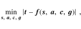
where
In Eq. (1) we distinguish between four categories
of parameters because of their different physical origins
and the way they appear in the equations. For example, each source
(distinguished by index i) has its own set of astrometric parameters,
represented by a sub-vector ![]() .
Similarly, while the instrument
attitude
(i.e., its precise spatial orientation with respect to a celestial reference
system)
is in principle a single continuous function of time, its
numerical representation is for practical reasons (data gaps, etc.)
subdivided into time segments (index j) with independent
attitude parameter sub-vectors
.
Similarly, while the instrument
attitude
(i.e., its precise spatial orientation with respect to a celestial reference
system)
is in principle a single continuous function of time, its
numerical representation is for practical reasons (data gaps, etc.)
subdivided into time segments (index j) with independent
attitude parameter sub-vectors ![]() .
The instrument calibration
(i.e., the precise
geometry of the optics and focal-plane assembly including the CCDs)
is also subdivided into units (index k), e.g., for the different
CCDs, with independent calibration parameter sub-vectors
.
The instrument calibration
(i.e., the precise
geometry of the optics and focal-plane assembly including the CCDs)
is also subdivided into units (index k), e.g., for the different
CCDs, with independent calibration parameter sub-vectors ![]() .
By definition, the global parameter vector is not similarly subdivided:
it contains parameters that affect all observations, such as the
parameterized post-Newtonian (PPN) parameter
.
By definition, the global parameter vector is not similarly subdivided:
it contains parameters that affect all observations, such as the
parameterized post-Newtonian (PPN) parameter ![]() (Hobbs et al. 2009).
(Hobbs et al. 2009).
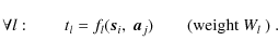
Each CCD observation l is therefore uniquely associated with a
specific object i, an attitude time segment j, and a calibration
unit k. This mapping is formally expressed by the functions
i(l), j(l), k(l).
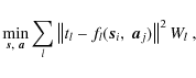
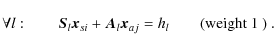
Adopting a weighted L2 (Euclidean) norm in Eq. (1),
the minimization problem can then be written

where Wl is the statistical weight associated with CCD observation l. Subsequently we assume that the weights are fixed and known.
The attitude parameters define the spatial orientation of the instrument as function of time, relative to the celestial reference system. For AGIS, the instantaneous attitude is represented by a unit quaternion (Wertz 1978), and the four components of the quaternion are represented as continuous functions of time by means of cubic spline functions on a (more or less regular) knot sequence. Since the quaternion is normalized to unit length, the model has three degrees of freedom per knot. In general, three independent quantities are needed to describe the orientation at any time, and we may assume that one of them to represent the rotational state around the satellite spin axis. Information about this (along-scan) attitude component is provided by the CCD observation times. Some of the CCD observations will give an additional measurement of the across-scan coordinate of the source image at the time of the observation. These observations are obtained with a lower accuracy than the along-scan (timing) observations, but are crucial for determination of the remaining two components of the attitude, representing orientation about two axes perpendicular to the spin axis. These measurements have to be included in the actual minimization problem (2), but they can be neglected here because they do not change the formal structure of the problem (i.e., they do not create additional links between the unknowns). For the present discussion it is useful to think of the instantaneous attitude as represented by three angles, one of which describing the along-scan orientation of the instrument and the other two being across-scan components of the attitude.
2.3 The simplified problem
In order to simplify the description of the astrometric problem,
we will subsequently assume that the instrument is perfectly
calibrated and that the global parameters are perfectly known,
so that in effect we can ignore ![]() and
and ![]() in
Eq. (1). The resulting simplified problem is therefore
in
Eq. (1). The resulting simplified problem is therefore
where, for conciseness, the dependence of i and j on l is not explicitly written out but is implied in this and the following equations.
There are several reasons for introducing the simplification of
neglecting ![]() and
and ![]() .
Concerning
the global parameters, they are typically of such a nature that they
can be considered known from first principles; e.g., the PPN parameter
.
Concerning
the global parameters, they are typically of such a nature that they
can be considered known from first principles; e.g., the PPN parameter
![]() according to General Relativity. Furthermore, there
are much fewer calibration (
according to General Relativity. Furthermore, there
are much fewer calibration (![]() )
and global parameters (
)
and global parameters (![]() )
than attitude (
)
than attitude (
![]() )
and source parameters
(
)
and source parameters
(
![]() for the primary sources). More importantly,
experience both from the Hipparcos reductions and simulated Gaia
data processing shows that the geometrical instrument calibration
(e.g., determination of the effective field distortion) is quite
straightforward and well separated from the determination of source
and attitude parameters (e.g., by accumulating a map of average
positional residuals across the field of view). The real
problem lies in separating the source and attitude parameters.
This can be qualitatively understood from a consideration of how
the calculated observation times depend on the different parameters.
Because each global or calibration parameter affects a very large
number of observations spread over the whole celestial sphere, or
a large part of it, its determination is not greatly affected by
localized errors related to the source and attitude parameters.
By contrast, both the attitude and source parameters may have a
very local influence function on the sky, which could render their
disentanglement more difficult (cf. van Leeuwen 2007, Sect. 1.4.6).
for the primary sources). More importantly,
experience both from the Hipparcos reductions and simulated Gaia
data processing shows that the geometrical instrument calibration
(e.g., determination of the effective field distortion) is quite
straightforward and well separated from the determination of source
and attitude parameters (e.g., by accumulating a map of average
positional residuals across the field of view). The real
problem lies in separating the source and attitude parameters.
This can be qualitatively understood from a consideration of how
the calculated observation times depend on the different parameters.
Because each global or calibration parameter affects a very large
number of observations spread over the whole celestial sphere, or
a large part of it, its determination is not greatly affected by
localized errors related to the source and attitude parameters.
By contrast, both the attitude and source parameters may have a
very local influence function on the sky, which could render their
disentanglement more difficult (cf. van Leeuwen 2007, Sect. 1.4.6).
One further reason for considering the simplified problem is that we want to study the feasibility of a direct solution of the least-squares problem. It is then necessary that an efficient direct algorithm should first work for the simplified problem. Adding the calibration and global parameters can only make the problem more difficult.
2.4 Observations (data) and unknowns (parameters)
The simplified least-squares problem involves three very large vectors:
![]() containing the observations (CCD observation times),
containing the observations (CCD observation times),
![]() containing the unknown source parameters, and
containing the unknown source parameters, and ![]() containing the unknown attitude parameters.
containing the unknown attitude parameters.
To give an idea of the number of observations and unknowns we give rough approximations based on the current (and final) Gaia design. Gaia will observe a total of about 109 objects, but only a fraction of them will be used for the astrometric solution, i.e., as ``primary sources''. (Astrometric parameters for other objects can be calculated off-line, one object at a time, once the attitude and calibration parameters have been determined by means of the primary sources.) The primary sources are selected iteratively for their astrometrically benign nature, e.g., avoiding all known or suspected double stars as well as sources showing unexpectedly large residuals in the astrometric solution. Apart from these constraints it is advantageous to use as many primary sources as possible because that will increase the accuracy of the instrument calibration and attitude determination. It is not known how many primary sources will eventually be used for Gaia, but a design goal for AGIS is to be able to handle at least 108 primary sources, covering the full range of magnitudes and colours, with a not too uneven distribution on the sky, and being observed throughout the duration of the mission.
Neglecting observational dead time, the average number of CCD observations
per object is directly given by the number of superposed fields (=2),
the number of astrometric CCDs that the object successively crosses
in each field of view (=9), the transverse (across-scan) size of
the field of view (
![]() ), the mission length (T=5 years),
and the satellite spin rate (
), the mission length (T=5 years),
and the satellite spin rate (![]() arcsec s-1). The result is
arcsec s-1). The result is
![]() CCD observations per
object. With n=108 primary sources the total number of observations is
CCD observations per
object. With n=108 primary sources the total number of observations is
![]() .
.
There are five astrometric parameters per primary source
(two components for the position at the reference epoch, one
for the parallax, and two proper motion components, Lindegren et al., in prep.);
hence
![]() .
.
The number of free attitude parameters depends on the adopted
attitude model. This, in turn, should be optimized by taking into
account the nature and level of perturbations on one hand, and the
number and quality of primary source observations on the other.
The new Hipparcos reduction (van Leeuwen 2007) used a dynamical
model of the satellite to reduce the number of attitude parameters
and hence improve the accuracy of the solution. For Gaia, the
attitude control using continuously active gas thrusters will introduce
high-frequency perturbations that make it meaningless to dynamically
predict the along-scan attitude motion over intervals longer than a
few seconds - after that the new observations are more accurate than
the prediction. This suggests that the attitude model should have
one degree of freedom per axis for every 10-20 s. With the adopted
(cubic) spline representation of the attitude components as functions
of time (see Sect. 2.2), and assuming a maximum knot
interval of about 20 s, the minimum number of scalar attitude
parameters for a 5-year mission is
![]() .
.
It is reasonable to ask whether cubic splines are the best choice for a direct solution. It might be that a different representation of the attitude could reduce the number of attitude unknowns, in particular if the noise level introduced by the control system is less than currently foreseen. However, splines have an important advantage from a computational viewpoint, namely that they are local in the sense that a change in the data at point t' has little effect on the fitted spline at t, provided that |t'-t| is large enough (typically spanning tens of knots). The use of a dynamical model or other approximation schemes is likely to cause a partial loss of this ``locality'', and it can be inferred from the present study that this would vastly modify the sparseness structure of the adjustment problem in the sense of making a direct solution even harder.
2.5 Observation equations
The weighted least-squares problem (3) corresponds
to the over-determined system of non-linear observation equations
Since the function fl is non-linear but smooth, we use a linear expansion around some suitable reference values
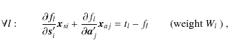
with fl and partial derivatives evaluated at the reference point
The choice of spline functions for representing the attitude has a direct influence on the structure of the observation equations (6) through the definition of
From Eq. (6) it is evident that observation equations
for different sources involve disjoint source parameter sub-vectors
![]() but may refer to the same attitude sub-vector
but may refer to the same attitude sub-vector ![]() .
Sorting all the observation Eqs. (6) by the source
index i and collecting them in one matrix we get a non-square block
angular matrix
.
Sorting all the observation Eqs. (6) by the source
index i and collecting them in one matrix we get a non-square block
angular matrix![]() (see Björck 1996):
(see Björck 1996):
![\begin{displaymath}
\left[\begin{array}{ccccc}
\vec{S}_{i=1} & 0 & \cdots & 0 ...
...y}\right]\;\; \Leftrightarrow \; \; \vec{M}\vec{x} = \vec{h} ,
\end{displaymath}](/articles/aa/full_html/2010/08/aa13503-09/img57.png)
with n the number of primary sources (108). The matrices
In Eqs. (6)-(7) and all following equations, it is
important to note our (slightly unconventional) use of indices in the subscripts.
Since index l is exclusively used for the observations, and i, j respectively
for the sources and attitude time segments, ![]() and
and ![]() signify
different matrices, even when the indices l and i happen to have
the same numerical value.
signify
different matrices, even when the indices l and i happen to have
the same numerical value. ![]() is the
is the ![]() matrix containing
the partial derivatives of fl with respect to the five astrometric parameters
of source number i(l), multiplied by the square root of the weight of
observation tl. Suppose that there are oi observations of source i.
matrix containing
the partial derivatives of fl with respect to the five astrometric parameters
of source number i(l), multiplied by the square root of the weight of
observation tl. Suppose that there are oi observations of source i.
![]() is then the
is then the
![]() matrix obtained by stacking
matrix obtained by stacking ![]() for every l such that i(l) = i. A similar distinction is made between
for every l such that i(l) = i. A similar distinction is made between
![]() ,
referring to observation l, and
,
referring to observation l, and ![]() ,
obtained by
stacking all
,
obtained by
stacking all ![]() for which i(l)=i.
for which i(l)=i.
For example, consider the source i=1 with o1=3 observations for l=7,
22 and 3999, each occurring at a different attitude interval with
index j=11, 123 and 200, respectively. Then
![\begin{displaymath}\vec{S}_{i=1}=
\left[
\begin{array}{c}
\vec{S}_{l=7} \\
\vec...
...c}
h_{l=7} \\
h_{l=22} \\
h_{l=3999} \\
\end{array}\right].
\end{displaymath}](/articles/aa/full_html/2010/08/aa13503-09/img66.png)
|
(8) |
and
![\begin{displaymath}\vec{A}_{i=1}=
\left[
\begin{array}{ccccccc}
\cdots & (j\!=\!...
...} & \cdots & \vec{A}_{l=3999} & \cdots \\
\end{array}\right],
\end{displaymath}](/articles/aa/full_html/2010/08/aa13503-09/img67.png)
|
(9) |
where the column indices of the three non-zero columns are shown in the top row. Note that
2.6 Normal equations
The system (7) is over-determined: there are more
equations than unknowns. Due to measurement errors, there does not
exist a solution that simultaneously satisfies all the equations.
However the problem becomes mathematically well posed when we try
to minimize the norm of the post-fit residual vector,
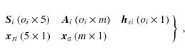
This is the ordinary least-squares problem, which is classically solved by forming the normal equations
or
![\begin{displaymath}
\left[\begin{array}{ccccc}
\vec{S}_1{'\!}\vec{S}_1 & 0 & \...
...]
\sum_i \vec{A}_i{'\!}\vec{h}_{si} \\
\end{array}\right] ,
\end{displaymath}](/articles/aa/full_html/2010/08/aa13503-09/img74.png)
where the prime (') denotes matrix transpose and the numerical subscripts refer to the source index i. The full normal equations matrix
Thanks to the scanning law of Gaia, and provided that a sufficient number
of sources are observed a sufficient number of times over the mission, it
is found that each of the diagonal sub-matrices
![]() and
and
![]() are positive-definite. Yet the
complete system (12) is in principle singular (although rounding
errors will in practice make it non-singular): it is expected to be
positive-semidefinite with rank 5n+m-6, owing to the circumstance that
all the observations are invariant with respect to the choice of celestial
reference system. The 6-dimensional nullspace is in fact well known and
corresponds to the undefined orientation and spin of the reference system
in which both the source parameters and the attitude are expressed. This
singularity is therefore of a benign nature and the associated numerical
difficulties can easily be overcome (Lindegren et al., in prep.). For simplicity we
subsequently ignore this particular feature of the problem and assume
that the normal matrix
are positive-definite. Yet the
complete system (12) is in principle singular (although rounding
errors will in practice make it non-singular): it is expected to be
positive-semidefinite with rank 5n+m-6, owing to the circumstance that
all the observations are invariant with respect to the choice of celestial
reference system. The 6-dimensional nullspace is in fact well known and
corresponds to the undefined orientation and spin of the reference system
in which both the source parameters and the attitude are expressed. This
singularity is therefore of a benign nature and the associated numerical
difficulties can easily be overcome (Lindegren et al., in prep.). For simplicity we
subsequently ignore this particular feature of the problem and assume
that the normal matrix ![]() is positive-definite.
is positive-definite.
2.7 Sparseness structure
In this section we investigate the sparseness structure of
the observation matrix ![]() and the normal matrix
and the normal matrix ![]() .
In linear algebra the sparseness notion refers to matrices or systems
of equations where only a (very small) fraction of the elements
have non-zero values. We use
.
In linear algebra the sparseness notion refers to matrices or systems
of equations where only a (very small) fraction of the elements
have non-zero values. We use
![]() to denote the
fill factor of the matrix
to denote the
fill factor of the matrix ![]() ,
i.e., the fraction
of non-zero elements. The sparseness structure of
the present equations is directly related to the design of Gaia: two
telescopes separated by a large fixed angle, orthogonal to a spin axis,
and a scanning law that has been optimized to maximize the sky coverage
within given technology constraints, leading to a satellite spin
period of 6 hr with a precession rate of approximately
,
i.e., the fraction
of non-zero elements. The sparseness structure of
the present equations is directly related to the design of Gaia: two
telescopes separated by a large fixed angle, orthogonal to a spin axis,
and a scanning law that has been optimized to maximize the sky coverage
within given technology constraints, leading to a satellite spin
period of 6 hr with a precession rate of approximately
![]() (see Lindegren et al. 2008).
(see Lindegren et al. 2008).
With
![]() denoting the number of observations of
source i and
denoting the number of observations of
source i and
![]() the number of attitude parameters,
the dimensions (rows
the number of attitude parameters,
the dimensions (rows![]() columns) of the various sub-matrices
in Eq. (7) are as follows:
columns) of the various sub-matrices
in Eq. (7) are as follows:
|
(13) |
For the normal equations (12) we have the dimensions:

|
(14) |
3 Direct solution method
In this section we consider the possibility of computing a direct (i.e., non-iterative and algebraically exact) solution to the normal Eqs. (12). Already in the early phases of the Hipparcos project it was concluded that a direct solution of the corresponding (much smaller) problem would not be feasible, and the so-called three-step procedure was invented as a practical, albeit approximate workaround (Sect. 5.3). Since then, the available storage and computing power have increased by many orders of magnitude and it is not obvious that even the much larger Gaia problem is intractable by a direct method. However, as we shall see below, it appears that the direct method is still quite unfeasible, although it may be difficult to prove such an assertion in full mathematical rigour.
Let us start with a few general observations. The solution of a non-sparse
system of normal equations with N unknowns in general requires a minimum
of about N3/6 floating-point operations
![]() ,
where an operation typically involves one
multiplication (or division) and one addition, plus some subscripting
(Golub & van Loan 1996). For a sparse matrix there is no general formula, since
the required effort depends critically on the detailed sparseness structure
(i.e., the connectivity amongst the unknowns), the ordering of the unknowns,
and the chosen solution algorithm. A lower bound is given by
,
where an operation typically involves one
multiplication (or division) and one addition, plus some subscripting
(Golub & van Loan 1996). For a sparse matrix there is no general formula, since
the required effort depends critically on the detailed sparseness structure
(i.e., the connectivity amongst the unknowns), the ordering of the unknowns,
and the chosen solution algorithm. A lower bound is given by
![]() ,
which applies to a banded matrix (George & Liu 1981).
Considering the normal matrix
,
which applies to a banded matrix (George & Liu 1981).
Considering the normal matrix ![]() in Eq. (12)
with
in Eq. (12)
with
![]() and
and
![]() this
gives operation counts from 1014 to a few times 1025 flop. It is
envisaged that the astrometric solution for Gaia will run on a computing
system with a performance of about 10 TFLOPS, or 1013 floating-point
operations per second (Lammers et al. 2009). Theoretically, this gives a computing
time of tens of seconds for the lower bound, and tens of thousands of years
for the upper bound, i.e., ranging from clearly feasible to clearly
unfeasible
this
gives operation counts from 1014 to a few times 1025 flop. It is
envisaged that the astrometric solution for Gaia will run on a computing
system with a performance of about 10 TFLOPS, or 1013 floating-point
operations per second (Lammers et al. 2009). Theoretically, this gives a computing
time of tens of seconds for the lower bound, and tens of thousands of years
for the upper bound, i.e., ranging from clearly feasible to clearly
unfeasible![]() . In order to refine the estimate we need
to specify the solution method more precisely and take a closer look
at the sparseness structure. In this section we consider a solution
based on the elimination of the source parameters, which seems the
most natural approach for the present problem. In Sect. 5
we briefly consider some possible alternative approaches to the direct
solution.
. In order to refine the estimate we need
to specify the solution method more precisely and take a closer look
at the sparseness structure. In this section we consider a solution
based on the elimination of the source parameters, which seems the
most natural approach for the present problem. In Sect. 5
we briefly consider some possible alternative approaches to the direct
solution.
3.1 Reduced normal matrix
A standard way to handle normal equations with the block-diagonal-bordered structure of Eq. (12) is to successively eliminate the unknowns along the block-diagonal (in our case the source parameters), leaving us with a ``reduced'' normal equations system for the remaining unknowns (in our case the attitude parameters). The gain is a huge reduction in the size of the system that has to be solved, at the expense of a much denser reduced matrix.
A straightforward computation shows that the solution of Eq. (12)
can be accomplished by first solving the reduced normal equations for the
attitude parameters,
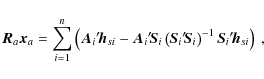
where
is the reduced normal matrix, and then forwarding the solution
This well-known computational trick, tantamount to a block-wise gaussian elimination, was used e.g. for the Hipparcos sphere solution (see ESA 1997, Vol. 3, p. 208) and is also used for the one-day astrometric solution as part of the Gaia first look processing (see Bombrun 2008a; Jordan et al. 2009; Bernstein et al. 2005). The initial problem has been reduced to a smaller one. For the global space astrometry problem, the complexity essentially consists of solving the reduced normal equations (15), which involves the sparse symmetric positive-definite matrix
3.2 Complexity of the Cholesky factorization
In order to solve Eq. (15), we investigate the Cholesky
factorization of the reduced normal matrix ![]() .
The Cholesky
factorization is a useful and well-known method
to solve linear equations involving a positive-definite matrix, see
Appendix B. Moreover, the complexity of this factorization,
which is strongly related to the sparseness structure of the matrix to be
factored, can easily be computed. In Appendix A we
present the sparseness structure of the reduced normal matrix.
As we are here only concerned with the complexity of the factorization,
not by the actual numerical values, we use symbolic computation. For
sparse matrices this means that the indices of non-zero elements occurring
during the computation are traced, which enables us to compute the number
of floating-point operations required for the factorization, as well as
the sparsity of the resulting factor.
.
The Cholesky
factorization is a useful and well-known method
to solve linear equations involving a positive-definite matrix, see
Appendix B. Moreover, the complexity of this factorization,
which is strongly related to the sparseness structure of the matrix to be
factored, can easily be computed. In Appendix A we
present the sparseness structure of the reduced normal matrix.
As we are here only concerned with the complexity of the factorization,
not by the actual numerical values, we use symbolic computation. For
sparse matrices this means that the indices of non-zero elements occurring
during the computation are traced, which enables us to compute the number
of floating-point operations required for the factorization, as well as
the sparsity of the resulting factor.
Even using symbolic computation, ![]() is far too large to be
easily studied in full. Instead we consider sequences of increasingly
larger submatrices that allow extrapolation to the full-size problem.
A principal submatrix of
is far too large to be
easily studied in full. Instead we consider sequences of increasingly
larger submatrices that allow extrapolation to the full-size problem.
A principal submatrix of ![]() is obtained by deleting a certain subset of the rows and the corresponding
columns. Since
is obtained by deleting a certain subset of the rows and the corresponding
columns. Since ![]() is symmetric and positive-definite, that is also
true of all its principal submatrices (Stewart 1998).
is symmetric and positive-definite, that is also
true of all its principal submatrices (Stewart 1998).
As explained in Sect. 2.4, the attitude parameters are grouped
in sub-vectors ![]() corresponding to non-overlapping time segments.
Deleting the rows and columns in
corresponding to non-overlapping time segments.
Deleting the rows and columns in ![]() for a certain time segment
is clearly equivalent to excluding all observations in that time
segment. Conversely, by considering only the observations in selected time
segments, we obtain a principal submatrix of
for a certain time segment
is clearly equivalent to excluding all observations in that time
segment. Conversely, by considering only the observations in selected time
segments, we obtain a principal submatrix of ![]() .
.
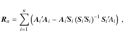
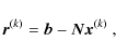
![\begin{figure}
\par\includegraphics[width=9cm,clip]{13503fg1}
\end{figure}](/articles/aa/full_html/2010/08/aa13503-09/img113.png)
|
Figure 1:
The fill factor |
| Open with DEXTER | |
Using the small-scale simulation software AGISLab (Holl et al. 2009), the
structures of various principal submatrices of ![]() were computed
for a problem with one million primary sources. Each complete rotation
(spin) of the satellite constitutes an attitude time segment of 6 h,
which is divided into 1000 knot intervals of
were computed
for a problem with one million primary sources. Each complete rotation
(spin) of the satellite constitutes an attitude time segment of 6 h,
which is divided into 1000 knot intervals of
![]() s.
For each pair of knot intervals,
s.
For each pair of knot intervals,
![]() ,
where
,
where ![]() and
and ![]() may belong to different time segments (spins), AGISLab provides the number
of sources observed in both intervals. If this number is not zero, then
the
may belong to different time segments (spins), AGISLab provides the number
of sources observed in both intervals. If this number is not zero, then
the ![]() block elements of the principal submatrix with
block elements of the principal submatrix with
![]() will be non-zero, where M=4 is the order of the
attitude spline (Sect. 2.5).
will be non-zero, where M=4 is the order of the
attitude spline (Sect. 2.5).
We consider three sequences of principal submatrices of ![]() ,
labelled set 1, 3 and 12, each covering up to 400 spins (j):
,
labelled set 1, 3 and 12, each covering up to 400 spins (j):

The number of spins included is successively increased to study the sparsity structure of the resulting principal submatrix. Symbolic Cholesky factorization was performed after a reordering of the attitude unknowns. We used the minimum degree algorithm and the reordering software Metis (Karypis & Kumar 1998), which implements one of the most efficient reordering algorithms. We also tried the reverse Cuthill-McKee algorithm (George & Liu 1981) but it is clearly less efficient than the minimum degree algorithm in terms of the sparseness of the resulting Cholesky factor.
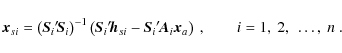
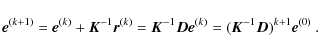
![\begin{figure}
\par\includegraphics[width=9cm,clip]{13503fg2}
\end{figure}](/articles/aa/full_html/2010/08/aa13503-09/img120.png)
|
Figure 2: Same as Fig. 1, but showing the complexity of reduced normal equations in terms of the number of floating-point operations (flop) needed to compute the Cholesky factors, using the minimum degree reordering algorithm and Metis software. |
| Open with DEXTER | |
Figure 1 shows the fill factors ![]() for the different
submatrices, and for the Cholesky factors after reordering using the
minimum degree algorithm, as functions of the total number of spins
considered. The full problem (5 yr) corresponds to about 7300 spins.
As shown by the lower set of curves in Fig. 1, the fill
factor for the principal submatrices of
for the different
submatrices, and for the Cholesky factors after reordering using the
minimum degree algorithm, as functions of the total number of spins
considered. The full problem (5 yr) corresponds to about 7300 spins.
As shown by the lower set of curves in Fig. 1, the fill
factor for the principal submatrices of ![]() decreases with the
number of spin rotations, although
it appears to level out at a few times 10-4. By contrast, for the
corresponding Cholesky factors the fill factor quickly approaches 1
(the upper set of curves),
implying that sparse matrix algorithms (including reordering) tend to
be useless when more than a few hundred spins are included.
decreases with the
number of spin rotations, although
it appears to level out at a few times 10-4. By contrast, for the
corresponding Cholesky factors the fill factor quickly approaches 1
(the upper set of curves),
implying that sparse matrix algorithms (including reordering) tend to
be useless when more than a few hundred spins are included.
Figure 2 shows the complexity of the solution in terms of the number of floating-point operations needed to compute the Cholesky factors, taking into account the sparseness. Also shown (by the upper, straight line) is the complexity of the Cholesky factorization of the corresponding full matrices. It is clear that the complexity of the sparse submatrices tends towards the upper bound for the full matrices.
Roughly speaking, the connectivity between the observations increases when more and more spins are included. Even if the submatrices tend to be sparser, it is not possible to break the increasing connectivity by reordering of the unknowns, at least not with the commonly used reordering algorithms. Hence, once Gaia has covered the whole sky, the Cholesky factor of the reduced normal matrix will be almost full and as difficult to compute as for a full matrix.
Extrapolating to the full size of the problem (7300 spins), we find
that a direct solution of the reduced normal equations (15)
will require about
![]() flop, the operation count for
the Cholesky decomposition of a full matrix of dimension
flop, the operation count for
the Cholesky decomposition of a full matrix of dimension ![]() ,
viz. m3/6.
,
viz. m3/6.
As explained in the introduction, we have deliberately ignored the calibration and global unknowns of the full Gaia adjustment problem. Both groups of unknowns will add more complexity and more fill-in. Similarly we have not discussed the numerical stability of a direct solution, and it is possible that a more refined numerical method, requiring an even greater computational effort than the Cholesky factorization, may be needed to compute an accurate solution. Moreover one should not forget about the complexity of storage. An upper triangular matrix with the dimension of the reduced normal matrix will require around 2 million Gigabytes. Operating efficiently on such a large matrix is certainly a very difficult problem in itself.
4 Iterative solution method
In this section we present the currently implemented iterative solution, AGIS (Lindegren et al., in prep.; O'Mullane et al., in prep.), adopting the simplifications of the present paper and comparing its complexity to that of the direct solution. The solution method outlined below belongs to a large and important class of iterative algorithms for the solution of sparse linear equations, known as Krylov subspace methods (van der Vorst 2003). The class includes well-known methods such as conjugate gradient which can be used for AGIS (Bombrun et al. in prep). The basic AGIS scheme described above is equivalent to the simplest of all Krylov subspace methods, appropriately termed ``simple iteration''.
4.1 The ``simple iterative'' scheme
In the present context, the iterative algorithm originally adopted
for the Gaia astrometric solution (AGIS) can be described as follows.
As in Eq. (11), let
![]() be the linear
system of equations to be solved, where
be the linear
system of equations to be solved, where ![]() is symmetric.
This system has the property that the matrix-vector product
is symmetric.
This system has the property that the matrix-vector product
![]() can be calculated rather easily, for arbitrary
can be calculated rather easily, for arbitrary ![]() ,
while the direct solution of
,
while the direct solution of
![]() is very difficult.
Now let
is very difficult.
Now let ![]() be some square matrix (``preconditioner'') of the same
size as
be some square matrix (``preconditioner'') of the same
size as ![]() ,
which in some sense approximates
,
which in some sense approximates ![]() ,
but has
the property that the system
,
but has
the property that the system
![]() can easily be
solved for arbitrary
can easily be
solved for arbitrary ![]() .
Writing
.
Writing
![]() (where
(where
![]() is sometimes called the ``defect'' matrix) the original
system becomes
is sometimes called the ``defect'' matrix) the original
system becomes
![]() ,
which naturally
leads to the iteration formula
,
which naturally
leads to the iteration formula![]()
for successive iterations
where
is the residual vector in the kth iteration. With
The algorithm converges to the correct solution if
The spectral radius of
The choice of preconditioner has a profound influence on
the rate of convergence in the simple iteration scheme. In analogy with
classical iteration schemes, using the diagonal (or block-diagonal)
part of the ![]() as preconditioner may be referred to as a
Jacobi iteration scheme, while the lower (block-) triangular part
of
as preconditioner may be referred to as a
Jacobi iteration scheme, while the lower (block-) triangular part
of ![]() is referred to as a Gauss-Seidel iteration scheme.
As shown below, AGIS is close to the classical Gauss-Seidel scheme
known to be a converging residual-reducing scheme
(Björck 1996, Sect. 7.3.2).
is referred to as a Gauss-Seidel iteration scheme.
As shown below, AGIS is close to the classical Gauss-Seidel scheme
known to be a converging residual-reducing scheme
(Björck 1996, Sect. 7.3.2).
4.2 Implementation in AGIS
The full normal Eqs. (12) can be written as
![\begin{displaymath}
\left[\begin{array}{cc}
\vec{N}_{ss} & \vec{N}_{sa} \\ [3p...
...y}{c}
\vec{b}_s \\ [3pt]
\vec{b}_a \\
\end{array} \right],
\end{displaymath}](/articles/aa/full_html/2010/08/aa13503-09/img146.png)
where
A natural choice to split the normals is therefore the following
Gauss-Seidel scheme:
![\begin{displaymath}
\vec{K} =
\left[ \begin{array}{cc}
\vec{N}_{ss} & \vec{\va...
...vec{\varnothing} & \vec{\varnothing} \\
\end{array}\right] ,
\end{displaymath}](/articles/aa/full_html/2010/08/aa13503-09/img156.png)
where each
where
The two steps (i) and (ii) exactly correspond to the source update and attitude update blocks of the original AGIS scheme, which therefore effectively implements the simple iteration with Gauss-Seidel preconditioner. The scheme is easily parallelizable, resulting in efficient and scalable software. The source and the attitude equations can even be accumulated in parallel, successively solved for each source, whereupon the updated source parameters are passed to the attitude equations. When all the sources have thus been processed, the attitude equations are ready to be solved.
4.3 Complexity of the iterative solution
In Sect. 3 we did not consider the complexity
of computing the normal matrix and the reduced normal matrix.
Indeed these computations are negligible compared with the
complexity of solving the reduced normal matrix. This is not
the case for the iterative method. For the present comparison,
let us assume that the calculation of a single observation
equation (i.e., of the observation residual and 5+3M=17partial derivatives) requires some p=104 flop. Assuming,
as in Sect. 2, n=108 sources,
![]() observations, and
observations, and
![]() attitude parameters, the complexity of building the source
part of the normal equations (25) is around
attitude parameters, the complexity of building the source
part of the normal equations (25) is around
![]() flop, while its solution and
updating of the source parameters only requires some
flop, while its solution and
updating of the source parameters only requires some
![]() flop. For the attitude part, assuming
that the residuals and partial derivatives are calculated
afresh (as is the case in AGIS), building the normal equations
in (26) requires around
flop. For the attitude part, assuming
that the residuals and partial derivatives are calculated
afresh (as is the case in AGIS), building the normal equations
in (26) requires around
![]() flop and another
flop and another
![]() flop for its solution.
Thus the total complexity per iteration is of the order of
flop for its solution.
Thus the total complexity per iteration is of the order of
![]() ,
by far dominated by the setting up of
the observation equations.
,
by far dominated by the setting up of
the observation equations.
We have seen that the complexity of one iteration of the
iterative method is much smaller than the complexity of
solving the full system. An additional question that needs
to be addressed then is the number of iterations needed
in order to obtain a good approximation to the solution
of the least squares problem. It is a drawback of any
iterative method over the direct method that a convergence
criterion must be set up, and there is in principle no
way to know in advance how many iterations are needed
to satisfy the criterion. For the present application, both
the full-scale AGIS implementation (Lindegren et al., in prep.;
O'Mullane et al., in prep.) and small-scale AGISLab experiments (Holl et al. 2009) indicate
that of the order of 100 simple iterations are required to
reach parameter updates that are negligible to the numerical
precision of the 64-bit arithmetics. This can be improved
by a moderate factor (2 to 4) by the use of slightly more
complex iteration schemes, including conjugate gradients
(Bombrun et al., in prep.). These schemes are not elaborated here since
they do not so much affect the complexity of each iteration.
The total complexity of the iterative solution is therefore
of the order of 1017 flop, or a factor
![]() smaller than the direct solution.
smaller than the direct solution.
5 Some alternative approaches to the direct solution
The scheme described in Sect. 3 is not the only possible way to obtain a direct solution, and in this section we briefly consider some alternative approaches.
5.1 Elimination of attitude parameters
As an alternative to eliminating the source parameters, we may consider
instead the elimination of the attitude parameters, one attitude segment
(j) at a time. This results in a reduced matrix ![]() for the
source parameters, of size
for the
source parameters, of size
![]() .
It consists of submatrices
of size
.
It consists of submatrices
of size ![]() ,
such that the (i,i')th submatrix is associated
with a pair of primary sources i and i'. The minimum fill factor can
easily be estimated from the geometry of the observations, submatrix
(i,i') being non-zero if and only if the two sources i and i'are observed in the same attitude interval at some point of the mission.
From the size of the fields of view of Gaia and the number of field
transits per source (cf. Sect. 2.4) it is found that
,
such that the (i,i')th submatrix is associated
with a pair of primary sources i and i'. The minimum fill factor can
easily be estimated from the geometry of the observations, submatrix
(i,i') being non-zero if and only if the two sources i and i'are observed in the same attitude interval at some point of the mission.
From the size of the fields of view of Gaia and the number of field
transits per source (cf. Sect. 2.4) it is found that
![]() ,
which is similar to the fill factor
found for the reduced attitude matrix
,
which is similar to the fill factor
found for the reduced attitude matrix ![]() (Fig. 1).
However, since for Gaia
(Fig. 1).
However, since for Gaia
![]() ,
while
,
while
![]() ,
the storage of
,
the storage of ![]() requires 2-3 orders of magnitude more memory than
requires 2-3 orders of magnitude more memory than ![]() .
We
have not studied the complexity of the Cholesky factorization of
.
We
have not studied the complexity of the Cholesky factorization of
![]() ,
but it seems likely that it is at least as large as that
of
,
but it seems likely that it is at least as large as that
of ![]() ,
and possibly several orders of magnitude larger.
This is based on the observations that the scanning law does not
admit any natural way of ordering the sources in order to reduce the
bandwidth of
,
and possibly several orders of magnitude larger.
This is based on the observations that the scanning law does not
admit any natural way of ordering the sources in order to reduce the
bandwidth of ![]() .
.
Given that ![]() for Gaia, elimination of the attitude parameters
thus appears to be much less advantageous than the scheme described
in Sect. 3, although it may potentially be interesting
for other missions involving a much smaller number of sources.
for Gaia, elimination of the attitude parameters
thus appears to be much less advantageous than the scheme described
in Sect. 3, although it may potentially be interesting
for other missions involving a much smaller number of sources.
5.2 Orthogonal transformation of the observation equations
Forming normal equations, that are then solved by means of a Cholesky
factorization, is generally speaking the most efficient direct way of
solving the linear least-squares problem (10), both in terms
of storage and
number of floating-point operations required. Numerically, however, it
is less stable and less accurate than some other methods that do not
form and operate on the normal equations. The basic reason for this is
that the condition number![]() of the normal equations matrix is the square of that of the observation
equations matrix, that is
of the normal equations matrix is the square of that of the observation
equations matrix, that is
![]() .
.
![]() is approximately the number of significant decimal
digits lost in computing the solution with finite-precision arithmetics.
Thus, a least-squares problem
with a moderately high condition number, say
is approximately the number of significant decimal
digits lost in computing the solution with finite-precision arithmetics.
Thus, a least-squares problem
with a moderately high condition number, say
![]() ,
could give a virtually useless solution in double-precision arithmetic
(
,
could give a virtually useless solution in double-precision arithmetic
(![]() 16 significant digits) if normal equations are used, while
a solution of the same observation equations using orthogonal transformation
could very well be viable. For this and related reasons, orthogonal
transformation methods are often strongly recommended for solving
least-squares problems. Compared with the normal equations approach,
the increase in the number of floating-point operations need not be
very high. For example, when Householder transformations are applied
to solve a non-sparse problem with many more observations than unknowns,
the increase in the operation counts is typically around a factor 2
(Björck 1996, Sect. 2.4).
16 significant digits) if normal equations are used, while
a solution of the same observation equations using orthogonal transformation
could very well be viable. For this and related reasons, orthogonal
transformation methods are often strongly recommended for solving
least-squares problems. Compared with the normal equations approach,
the increase in the number of floating-point operations need not be
very high. For example, when Householder transformations are applied
to solve a non-sparse problem with many more observations than unknowns,
the increase in the operation counts is typically around a factor 2
(Björck 1996, Sect. 2.4).
Fortunately, the Gaia astrometric problem is well-conditioned by
design, so the superior numerical properties of orthogonal
transformation methods are not necessarily a strong argument in
their favour. A more important argument could be that the observation
equations have a vastly simpler structure than the normal equations.
If this can somehow be taken advantage of in the solution process,
it could potentially lead to significant savings in terms of storage
and flop. The standard approach is the QR factorization, which uses
a sequence of orthogonal transformations to decompose the observation
equations matrix as
![]() ,
where
,
where ![]() is
orthogonal and
is
orthogonal and ![]() is upper triangular
is upper triangular![]() .
The application of the QR factorization to a block angular matrix
as in Eq. (7) is described for example in Sect. 6.3
of Björck (1996). Briefly, for each source (i) the observation
Eqs. (6), here summarized by
.
The application of the QR factorization to a block angular matrix
as in Eq. (7) is described for example in Sect. 6.3
of Björck (1996). Briefly, for each source (i) the observation
Eqs. (6), here summarized by
![]() ,
are first reduced to upper triangular form by
the orthogonal transformation
,
are first reduced to upper triangular form by
the orthogonal transformation
![\begin{displaymath}
\vec{Q}_i'
\left[\begin{array}{ccc}
\vec{S}_i & \vec{A}_i &...
...ec{\varnothing} & \vec{T}_i & \vec{d}_{i}
\end{array}\right] ,
\end{displaymath}](/articles/aa/full_html/2010/08/aa13503-09/img192.png)
where
![\begin{displaymath}
\vec{Q}_a'
\left[\begin{array}{cc}
\vec{T}_1 & \vec{d}_1 \\ ...
..._a\\ [3mm]
\vec{\varnothing} & \vec{d}_a
\end{array} \right] .
\end{displaymath}](/articles/aa/full_html/2010/08/aa13503-09/img197.png)
The original least-squares problem is then equivalent to solving the system for the attitude unknowns,
5.3 Hipparcos-type decomposition
For completeness we mention here also the astrometric solution
method adopted for the original reduction of the Hipparcos
data by the two data analysis consortia, FAST (Kovalevsky et al. 1992)
and NDAC (Lindegren et al. 1992). The astrometric solution for
Hipparcos involved about
![]() observations of
observations of
![]() sources (stars), and
sources (stars), and
![]() attitude parameters.
Already in the very early mission studies (in the 1970's) it
was realized that the complexity of the astrometric solution
would be daunting; for example, a comparison with the then
recently developed photographic plate overlap reduction
technique (Jefferys 1979; Eichhorn 1960; Jefferys 1963) gave
estimates of
attitude parameters.
Already in the very early mission studies (in the 1970's) it
was realized that the complexity of the astrometric solution
would be daunting; for example, a comparison with the then
recently developed photographic plate overlap reduction
technique (Jefferys 1979; Eichhorn 1960; Jefferys 1963) gave
estimates of
![]() floating-point operations
(flop).
This basically assumed
a solution based on the approach in Sect. 5.1,
viz., that the attitude unknowns were first eliminated,
leading to a nearly full, reduced normal equations matrix
floating-point operations
(flop).
This basically assumed
a solution based on the approach in Sect. 5.1,
viz., that the attitude unknowns were first eliminated,
leading to a nearly full, reduced normal equations matrix
![]() of dimension
of dimension
![]() .
Its Cholesky decomposition
would require
.
Its Cholesky decomposition
would require
![]() flop.
flop.
The so-called three-step method was proposed by Lindegren in 1976 (unpublished) as a practical way to achieve a solution with only marginal degradation compared with a theoretically optimum solution (ESA 1997, Vol. 3, Sect. 4.1). The three steps are:
- 1.
- The ``great-circle reduction'' uses observations in a few consecutive spins to solve the one-dimensional positions (``abscissae'') of the sources along a reference great circle, together with the relevant attitude and calibration parameters. The origin (zero point) of the abscissae along the reference great circle is arbitrary in each such solution.
- 2.
- The ``sphere solution'' uses all the abscissae from Step 1
as ``observations'' for a least-squares solution of the
abscissa zero points. The observation equations also involve
the five astrometric parameters per source, but they can be
eliminated successively (analogous to the calculation of
 in Sect. 3.1). The resulting
system for the abscissa zero points is nearly full, and
can be solved by standard methods.
in Sect. 3.1). The resulting
system for the abscissa zero points is nearly full, and
can be solved by standard methods.
- 3.
- The ``astrometric parameter determination'' is a back-substitution of the abscissa zero points from Step 2 into the observation equations for the individual sources. The resulting least-squares systems, analogous to Eq. (17), were solved one source at a time to give the source parameters.
The three-step method appears simple and logical in view of the scanning law and basic one-dimensionality of the measurements (both for Hipparcos and Gaia). Moreover, it has been shown to work in practice for Hipparcos. It may therefore be of some interest to examine the approximations involved in it, and why it has not been adopted for Gaia.
The use of one-dimensional abscissae as an intermediate step is clearly an approximation in the sense that the information contained in the perpendicular coordinate (``ordinate'') is ignored. Moreover, since the instantaneous scanning circle can be inclined with respect to the reference great circle by up to a few degrees, initial errors in the source ordinates, and the corresponding attitude errors, effectively add some (much smaller) along-scan observation errors, due to their projection onto the instantaneous scanning circle. This makes it necessary to iterate the three-step procedure at least a few times, as was actually done for the Hipparcos reductions.
However, the restriction of the intermediate data to one-dimensional abscissae is not a fundamental one. Indeed, it is possible to use two-dimensional positions (albeit with a highly anisotropic precision), as in the so-called Ring Solution, also called the one day astronomical solution, of the Gaia First-Look Processing (Bombrun 2008a; Jordan et al. 2009; Bernstein et al. 2005), or even five-dimensional data, using the full parametrization of the primary sources, by a slight generalization of the method.
The abscissae in the Hipparcos great-circle solution, and the
two-dimensional positions in the Ring Solution, are somewhat
akin to the ``normal places'' (Normalorte in German)
often encountered especially in older astronomical literature,
e.g., for least-squares determination of the orbits of asteroids,
comets and visual binaries. The basic idea is that multiple
observations, usually obtained in a limited time interval,
can be grouped together, and subsequently treated as a single
observation with the combined weight of the individual
observations. When considering a single coordinate (e.g.,
declination, ![]() )
the method amounts to computing a
weighted mean of a group of residuals
)
the method amounts to computing a
weighted mean of a group of residuals
![]() with
respect to some reference orbit, and then treating this
mean residual as an observation referring to the weighted
mean time of observation within the group
(von Oppolzer 1880, p. 371). This can greatly reduce the
amount of computation needed to process long series of
observations, and the method of normal places was understandably
popular before the advent of electronic computers. In the
present context, a generalization of the method might be
relevant for reducing the amount of computation needed to
obtain the Gaia astrometric solution. The method is conveniently
discussed in terms of Ring Solutions (roughly corresponding
to Step 1 above) producing multiple two- or higher-dimensional
normal places for each source, and a single Ring-to-Sphere
solution putting all the normal places on a common reference
system (roughly corresponding to a combination of Step 2 and
3 above).
with
respect to some reference orbit, and then treating this
mean residual as an observation referring to the weighted
mean time of observation within the group
(von Oppolzer 1880, p. 371). This can greatly reduce the
amount of computation needed to process long series of
observations, and the method of normal places was understandably
popular before the advent of electronic computers. In the
present context, a generalization of the method might be
relevant for reducing the amount of computation needed to
obtain the Gaia astrometric solution. The method is conveniently
discussed in terms of Ring Solutions (roughly corresponding
to Step 1 above) producing multiple two- or higher-dimensional
normal places for each source, and a single Ring-to-Sphere
solution putting all the normal places on a common reference
system (roughly corresponding to a combination of Step 2 and
3 above).
A closer examination of the procedure reveals several weaknesses. They are all related to the circumstance that each Ring Solution must use only observations in a limited time interval (hours to days). One weakness concerns the availability of positional information for the across-scan attitude determination. Normally this information would come primarily from scans making a large angle to the present scan, i.e., from other time intervals. Restricting the processing to data within a limited time interval will always entail a loss of positional information for the attitude determination. Another weakness is that instrument parameters that are constant on time scales longer than a Ring Solution cannot easily be correctly treated in the Ring Solutions. Further weaknesses are the arbitrariness of the division of the time line into Ring Solutions, and the absence of continuity at the times of division. Obviously, all these weaknesses can be eliminated by extending the Ring Solution to encompass the whole mission; this is however equivalent to the previously studied direct solution. Thus it appears that decomposition methods of this kind are always sub-optimal, to some extent arbitrary, and in any case requires iteration to propagate information back from the Ring-to-Sphere solution to the Ring Solutions. Although a viable solution along these lines could no doubt be found, it is difficult to see any real advantages over an iterative solution of the rigorous normal equations, as discussed in Sect. 4.
6 Conclusions
We have analyzed the structure of the least-squares problem
to simultaneously determine the astrometric parameters
(position, parallax, proper motion) of a large number of sources
and the three-axis attitude of a scanning satellite, with
application to the Gaia mission. Although the resulting normal
matrix is very sparse, its structure is complex and related to
the specific design of Gaia's instrument and scanning law. For
simplicity only
two kinds of unknowns were considered, viz., the source parameters
(
![]() )
and the attitude parameters
(
)
and the attitude parameters
(
![]() ). Eliminating either kind results in a
reduced normal matrix, and we have studied the smaller of them
(for the attitude parameters) in detail using numerical simulations
and symbolic
computation. Although the reduced attitude matrix is still sparse,
Cholesky decomposition gives a high degree of fill-in even after
re-ordering the unknowns. In particular, we have seen that the
minimum-degree re-ordering algorithm is not efficient to solve
this problem. Some alternative approaches to the direct solution
(eliminating the attitude unknowns, and orthogonal transformation
of the observation equations) have also been briefly considered,
but appear to be at least as complex.
These findings make it unlikely that any direct
method can be found to solve the overall Gaia astrometric adjustment
problem with current practical limitations in terms of storage and
floating-point operations. By comparison, a simple iteration scheme
requires negligible storage and a factor
). Eliminating either kind results in a
reduced normal matrix, and we have studied the smaller of them
(for the attitude parameters) in detail using numerical simulations
and symbolic
computation. Although the reduced attitude matrix is still sparse,
Cholesky decomposition gives a high degree of fill-in even after
re-ordering the unknowns. In particular, we have seen that the
minimum-degree re-ordering algorithm is not efficient to solve
this problem. Some alternative approaches to the direct solution
(eliminating the attitude unknowns, and orthogonal transformation
of the observation equations) have also been briefly considered,
but appear to be at least as complex.
These findings make it unlikely that any direct
method can be found to solve the overall Gaia astrometric adjustment
problem with current practical limitations in terms of storage and
floating-point operations. By comparison, a simple iteration scheme
requires negligible storage and a factor
![]() less
computations, and is clearly feasible. Alternative solution methods,
along the lines of the Hipparcos three-step procedure, involve
undesirable approximations without offering any clear advantages.
less
computations, and is clearly feasible. Alternative solution methods,
along the lines of the Hipparcos three-step procedure, involve
undesirable approximations without offering any clear advantages.
It should be stressed that the present results do not prove that a direct method is unfeasible. Indeed, even if it appears unlikely, it cannot be excluded that a good permutation of the unknowns can be found that dramatically reduces the fill-in of the Cholesky factor. Nonetheless, our conclusions support the current plans to implement relatively straightforward iteration schemes for the core astrometric solution of Gaia (Lindegren et al., in prep.). Their optimization is the subject of a separate paper (Bombrun et al., in prep.).
AcknowledgementsThis work was supported by the European Marie-Curie research training network ELSA (contract MRTN-CT-2006-033481) and by the Swedish National Space Board. The first author thanks Ulrich Bastian and Hans Bernstein for their useful comments on earlier versions of this paper (Bombrun 2008b).
Appendix A: Sparseness structure of the reduced normal matrix
In this appendix we give some more details concerning the
structure of the reduced normal matrix ![]() (Eq. (16)) computed by the process described
in Sect. 3.
(Eq. (16)) computed by the process described
in Sect. 3.
![\begin{figure}
\par\mbox{\includegraphics[width=8cm,clip]{13503fg3a.eps}\hspace{5mm}
\includegraphics[width=7.8cm,clip]{13503fg3b.eps} }
\end{figure}](/articles/aa/full_html/2010/08/aa13503-09/img211.png)
|
Figure A.1:
Left: Structure of the reduced normal matrix |
| Open with DEXTER | |
Figure A.1 (left) shows the sparseness structure of
the reduced normal matrix calculated from simulated Gaia observations
covering a period of 2.5 days (10 successive spins). Non-zero values
are filled and the zeroes left blank. This figure is similar to
Fig. 3 in Bernstein et al. (2005) and some figures in Bombrun (2008b). We can observe the effects of
the Gaia design. The two fields of view and the scanning law
introduce a banded, almost periodic, pattern. The first and
second bands parallel to the diagonal are due to connections
introduced by sources successively seen in the two fields of
view, whereas the third band is due to connections over a
full spin period (6 h). The distance between the diagonal
and the third band corresponds to a full rotation (![]() )
of Gaia around its spin axis, whereas the distance between the
diagonal and the first band corresponds to the basic angle between
the two fields of view (
)
of Gaia around its spin axis, whereas the distance between the
diagonal and the first band corresponds to the basic angle between
the two fields of view (
![]() ). Moreover, we observe that
the farther away from the diagonal a band is, the sparser is
becomes. This is due to the spin axis slowly changing its
direction, by about
). Moreover, we observe that
the farther away from the diagonal a band is, the sparser is
becomes. This is due to the spin axis slowly changing its
direction, by about ![]() per spin period. Some points
on the celestial sphere are repeatedly observed during more
than a day, whereas others are only observed in a single
passage of one of the fields of view.
per spin period. Some points
on the celestial sphere are repeatedly observed during more
than a day, whereas others are only observed in a single
passage of one of the fields of view.
In the right diagram of Fig. A.1 we plot an isolated pattern that appears in the reduced normal matrix some distance away from the diagonal. This pattern is composed of eight blocks of points. In order to understand this pattern, we should look at it as composed of two squares, one following the other in time, i.e., in the diagonal direction. On the time scale of a spin period (6 h), Gaia will scan the celestial sphere roughly along a great circle. Considering any two points in time during the mission, there are two such great circles (A and B in Fig. B.1) which usually intersect at a significant angle. This means that they only have common sources in two small areas (N1, N2) symmetrically with respect to the center of the celestial sphere. The sources at N1 link the attitude parameters around times A1, A2, B1 and B2. In Fig. B.1, the pointings A1, A2, B1 and B2 show the positions of the instrument x axis (half-way between the two fields of view) at these times. In Fig. A.1 (right) the corresponding connections are seen as the four groups of non-zero elements forming the corners of a square. Similarly, the sources around N2 link the attitude parameters around times A3, A4, B3 and B4 forming a second square in the diagram.
Although the approximate size and repetition period of the pattern shown in the right part of Fig. A.1 are determined by the angle between the two fields of view and the spin period, the pattern is not repeated with strict periodicity, due to the precessional motion of the spin axis around the Sun-Earth axis, which itself is rotating. Over the time, the spinning axis is again pointing toward one of its previous directions. Hence, far away from the diagonal, the pattern can become similar to the structure observed close to the diagonal. It may also happen that the non-zero bands are orthogonal, rather than parallel to the diagonal, viz., when the spin axis is pointing in the opposite direction. The complexity of the Cholesky decomposition (see Appendix B) of the reduced normal matrix is due to this particular structure that strongly connects all the attitude parameters over the whole mission.
Appendix B: Cholesky factorization and the Minimum Degree algorithm
![\begin{figure}
\par\includegraphics[width=6cm,clip]{13503fg4.eps}
\end{figure}](/articles/aa/full_html/2010/08/aa13503-09/img214.png)
|
Figure B.1:
Illustration of the two great-circle scans (A, B)
that may produce a connectivity diagram similar to the right graph
in Fig. A.1.
The two circles intersect at the nodes N1 and N2. The points marked
A1, A2, A3, A4 are successive pointings of the instrument x axis
(bisecting the two viewing directions) along scan A when either
N1 or N2 is observed in one of the fields of view. The angle from
N1 to A1 or A2 is half the basic angle,
|
| Open with DEXTER | |
Any real symmetric positive semidefinite matrix ![]() (i.e.,
(i.e.,
![]() is such that
is such that
![]() for all
vectors
for all
vectors ![]() )
can be factored into
)
can be factored into
![]() ,
where
,
where ![]() is a real, upper triangular matrix. The factorization
is achieved by means of the Cholesky algorithm
(e.g., Björck 1996; Golub & van Loan 1996; Stewart 1998). Cholesky
factorization is particularly useful for least-squares problems, where
the normal matrix
is a real, upper triangular matrix. The factorization
is achieved by means of the Cholesky algorithm
(e.g., Björck 1996; Golub & van Loan 1996; Stewart 1998). Cholesky
factorization is particularly useful for least-squares problems, where
the normal matrix ![]() is always symmetric positive semidefinite.
After factorization, the normal equations
is always symmetric positive semidefinite.
After factorization, the normal equations
![]() are
solved as the two triangular system
are
solved as the two triangular system
![]() and
and
![]() .
The factorization can be made ``in place'',
which means that the elements in (the upper triangular part of)
.
The factorization can be made ``in place'',
which means that the elements in (the upper triangular part of) ![]() are successively replaced by the elements of
are successively replaced by the elements of ![]() .
During this
process elements in
.
During this
process elements in ![]() that are strictly zero may be replaced
by non-zero elements in
that are strictly zero may be replaced
by non-zero elements in ![]() .
This is known as ``fill-in''. Thus,
factorization of a sparse matrix
.
This is known as ``fill-in''. Thus,
factorization of a sparse matrix ![]() usually results in a less
sparse triangular factor
usually results in a less
sparse triangular factor ![]() .
However, certain sparseness
structures of
.
However, certain sparseness
structures of ![]() (e.g., a band-diagonal structure) do not
produce fill-in when computing the Cholesky factor.
(e.g., a band-diagonal structure) do not
produce fill-in when computing the Cholesky factor.
It is important to note that the fill-in of the Cholesky factor ![]() depends on the order of the unknowns. Any reordering of the unknowns can
be formally represented by an orthogonal permutation matrix
depends on the order of the unknowns. Any reordering of the unknowns can
be formally represented by an orthogonal permutation matrix ![]() such
that
such
that
![]() is the vector of the reordered unknowns. The permuted
normal equations are
is the vector of the reordered unknowns. The permuted
normal equations are
![]() .
The permuted normal matrix,
.
The permuted normal matrix,
![]() ,
is obtained by reordering
both the rows and columns of
,
is obtained by reordering
both the rows and columns of ![]() ,
and is also symmetric positive
semidefinite, and can be factorized by the Cholesky algorithm.
,
and is also symmetric positive
semidefinite, and can be factorized by the Cholesky algorithm.
The fill-in of the Cholesky factor thus depends on ![]() .
In particular,
there is a permutation that minimizes the number of non-zero elements in
.
In particular,
there is a permutation that minimizes the number of non-zero elements in
![]() .
The computation of the best permutation matrix
.
The computation of the best permutation matrix ![]() is an
NP-complete problem (Cook 1971; Pothen 1988), i.e., a problem with a complexity that
grows faster than any polynomial in the size of the matrix
is an
NP-complete problem (Cook 1971; Pothen 1988), i.e., a problem with a complexity that
grows faster than any polynomial in the size of the matrix ![]() .
Since
no ``fast'' algorithm is known for this problem, essentially all permutations
have to be tested in order to find the one that minimizes the fill-in of the
Cholesky factor. This is not very meaningful, however, since it will take
less resources to solve the normal equations without reordering than to
find the best permutation.
.
Since
no ``fast'' algorithm is known for this problem, essentially all permutations
have to be tested in order to find the one that minimizes the fill-in of the
Cholesky factor. This is not very meaningful, however, since it will take
less resources to solve the normal equations without reordering than to
find the best permutation.
The Minimum Degree algorithm (Markowitz 1957) is a classical heuristic
process that computes a reordering of ![]() that decreases the
fill-in of the Cholesky factor. This reordering is not the best, but
is usually a good one. The idea of the minimum degree reordering is
to consider the graph of the sparseness structure and to perform at
each step the Gauss pivoting on the node with the minimum number
of direct connections with other nodes. For more information about the
minimum degree reordering, see for example Sect. 6.5.2 of Björck (1996)
and the description of the Matlab command symamd in
Davis (2006).
that decreases the
fill-in of the Cholesky factor. This reordering is not the best, but
is usually a good one. The idea of the minimum degree reordering is
to consider the graph of the sparseness structure and to perform at
each step the Gauss pivoting on the node with the minimum number
of direct connections with other nodes. For more information about the
minimum degree reordering, see for example Sect. 6.5.2 of Björck (1996)
and the description of the Matlab command symamd in
Davis (2006).
References
- Bastian, U., & Biermann, M. 2005, A&A, 438, 745 [NASA ADS] [CrossRef] [EDP Sciences] [Google Scholar]
- Bernstein, H., Bastian, U., & Hirte, S. 2005, Gaia Technical Notes, GAIA-ARI-BST-001-5 [Google Scholar]
- Björck, Å. 1996, Numerical Methods for Least Squares Problems (Philadelphia, PA, USA: Society for Industrial and Applied Mathematics) [Google Scholar]
- Bombrun, A. 2008a, Gaia Technical Notes, GAIA-ARI-APB-002 [Google Scholar]
- Bombrun, A. 2008b, Gaia Technical Notes, GAIA-ARI-APB-001 [Google Scholar]
- Cook, S. 1971, in Third Annual ACM Symposium on the Theory of Computing, 151 [Google Scholar]
- Davis, T. A. 2006, Direct Methods for Sparse Linear Systems (Fundamentals of Algorithms 2) (Philadelphia, PA, USA: Society for Industrial and Applied Mathematics) [Google Scholar]
- de Boor, C. 1978, A practical guide to splines (New York: Springer-Verlag) [Google Scholar]
- Eichhorn, H. 1960, Astron. Nachr., 285, 233 [Google Scholar]
- ESA. 1997, The Hipparcos and Tycho Catalogues, SP-1200 (ESA) [Google Scholar]
- George, A., & Liu, J. W.-H. 1981, Computer Solution of Large Sparse Positive Definite Systems (New Jersey: Prentice-Hall) [Google Scholar]
- Golub, G. H., & van Loan, C. F. 1996, Matrix computations, 3rd ed. (Baltimore: The Johns Hopkins University Press) [Google Scholar]
- Hobbs, D., Holl, B., Lindegren, L., et al. 2009, in IAU Symp. 261, ed. S. A. Klioner, P. K. Seidelmann, & M. Soffel, 320 [Google Scholar]
- Holl, B., Hobbs, D., & Lindegren, L. 2009, in IAU Symp. 261, ed. S. A. Klioner, P. K. Seidelmann, & M. Soffel, 892 [Google Scholar]
- Jefferys, W. H. 1963, AJ, 68, 111 [NASA ADS] [CrossRef] [Google Scholar]
- Jefferys, W. H. 1979, AJ, 84, 1775 [NASA ADS] [CrossRef] [Google Scholar]
- Jordan, S. 2008, Astron. Nachr., 329, 875 [Google Scholar]
- Jordan, S., Bastian, U., & Löffler, W. 2009, Gaia Technical Notes, GAIA-ARI-SJ-009-01 [Google Scholar]
- Karypis, G., & Kumar, V. 1998, SIAM J. Sci. Comput., 20, 359 [CrossRef] [MathSciNet] [Google Scholar]
- Kovalevsky, J., Falin, J. L., Pieplu, J. L., et al. 1992, A&A, 258, 7 [NASA ADS] [Google Scholar]
- Lacroute, P. 1967, Transactions of the IAU, XIIIB, 63 [Google Scholar]
- Lacroute, P. 1975, in Space Astrometry, ESRO SP-108, ed. T. D. Nguyen, & B. T. Battrick, 5 [Google Scholar]
- Lammers, U., Lindegren, L., O'Mullane, W., & Hobbs, D. 2009, in Astronomical Society of the Pacific Conference Series, ed. D. A. Bohlender, D. Durand, & P. Dowler, ASP Conf. Ser., 411, 55 [Google Scholar]
- Lindegren, L., Babusiaux, C., Bailer-Jones, C., et al. 2008, in IAU Symp. 248, ed. W. J. Jin, I. Platais, & M. A. C. Perryman, 217 [Google Scholar]
- Lindegren, L., Høg, E., van Leeuwen, F., et al. 1992, A&A, 258, 18 [NASA ADS] [Google Scholar]
- Markowitz, H. M. 1957, Management Sci., 3, 255 [CrossRef] [Google Scholar]
- Mignard, F., Bailer-Jones, C., Bastian, U., et al. 2008, in IAU Symp. 248, ed. W. J. Jin, I. Platais, & M. A. C. Perryman, 224 [Google Scholar]
- Perryman, M. A. C., de Boer, K. S., Gilmore, G., et al. 2001, A&A, 369, 339 [NASA ADS] [CrossRef] [EDP Sciences] [Google Scholar]
- Pothen, A. 1988, Technical report CS-88-16 [Google Scholar]
- Stewart, G. 1998, Matrix Algorithms: Basic decompositions (SIAM) [Google Scholar]
- van der Vorst, H. 2003, Iterative Krylov Methods for Large Linear Systems (Cambridge University Press) [Google Scholar]
- van Leeuwen, F. 2007, Hipparcos, the New Reduction of the Raw Data (Astrophysics and Space Science Library), 350 [Google Scholar]
- von Oppolzer, T. 1880, Lehrbuch zur Bahnbestimmung der Kometen und Planeten. Zweiter Band (Leipzig: Wilhelm Engelmann) [Google Scholar]
- Wertz, J. R. 1978, Spacecraft Attitude Determination and Control, 1st edn. (Kluwer Academic Publishers) [Google Scholar]
Footnotes
- ... solution
![[*]](/icons/foot_motif.png)
- Standard errors and correlations can nevertheless be estimated through statistical techniques, see Holl et al. (2009) for a first study of spatial correlations in the global astrometric solution for Gaia.
- ... matrix
- Also called Helmert blocking in reference to the German geodesist F. R. Helmert who described this structure in 1880.
- ...
- A floating-point is a standard that defines the representation of rational numbers in a computer. The term flop is used as a unit for the number of floating-point operations needed to solve a problem.
- ...
unfeasible
- For comparison, it is estimated that the entire Gaia DPAC processing will require of the order of 1021 flop (Mignard et al. 2008), comparable to several other large computational projects. On a 10 TFLOPS machine, the corresponding computing time is three years.
- ... formula
- In this and subsequent formulae, an expression like
 is shorthand notation for the solution of
 .
Naturally, the inverse matrix is never computed
unless explicitly needed.
.
Naturally, the inverse matrix is never computed
unless explicitly needed.
- ... number
- The condition number of the arbitrary (square or
rectangular)
matrix
 is defined in terms of the Euclidean matrix norm as
 ,
where
,
where
 is the pseudo-inverse of (e.g.,
Stewart 1998).
is the pseudo-inverse of (e.g.,
Stewart 1998).
- ... triangular
- The standard notation uses
 for the upper-triangular
matrix; hence the name QR factorization. For consistency with
Appendix B
and to avoid confusion with the reduced
matrix, we use
for the upper-triangular
matrix; hence the name QR factorization. For consistency with
Appendix B
and to avoid confusion with the reduced
matrix, we use  instead.
All Figures
|
|
Figure 1:
The fill factor |
| Open with DEXTER | |
| In the text | |
|
|
Figure 2: Same as Fig. 1, but showing the complexity of reduced normal equations in terms of the number of floating-point operations (flop) needed to compute the Cholesky factors, using the minimum degree reordering algorithm and Metis software. |
| Open with DEXTER | |
| In the text | |
|
|
Figure A.1:
Left: Structure of the reduced normal matrix |
| Open with DEXTER | |
| In the text | |
|
|
Figure B.1:
Illustration of the two great-circle scans (A, B)
that may produce a connectivity diagram similar to the right graph
in Fig. A.1.
The two circles intersect at the nodes N1 and N2. The points marked
A1, A2, A3, A4 are successive pointings of the instrument x axis
(bisecting the two viewing directions) along scan A when either
N1 or N2 is observed in one of the fields of view. The angle from
N1 to A1 or A2 is half the basic angle,
|
| Open with DEXTER | |
| In the text | |
Copyright ESO 2010
Current usage metrics show cumulative count of Article Views (full-text article views including HTML views, PDF and ePub downloads, according to the available data) and Abstracts Views on Vision4Press platform.
Data correspond to usage on the plateform after 2015. The current usage metrics is available 48-96 hours after online publication and is updated daily on week days.
Initial download of the metrics may take a while.