| Issue |
A&A
Volume 516, June-July 2010
|
|
|---|---|---|
| Article Number | A89 | |
| Number of page(s) | 15 | |
| Section | Extragalactic astronomy | |
| DOI | https://doi.org/10.1051/0004-6361/200912579 | |
| Published online | 20 July 2010 | |
A non-hydrodynamical model for acceleration of line-driven winds in active galactic nuclei
G. Risaliti1,2 - M. Elvis2
1 - INAF - Osservatorio Astrofisico di Arcetri, Largo E. Fermi 5, 50125
Firenze, Italy
2 - Harvard-Smithsonian Center for Astrophysics, 60 Garden Street, Cambridge, MA 02138, USA
Received 26 May 2009 / Accepted 4 November 2009
Abstract
Context. Radiation driven winds are the likely origin of AGN
outflows, and are believed to be a fundamental component of the inner
structure of AGNs. Several hydrodynamical models have been developed,
showing that these winds can be effectively launched from AGN accretion
disks.
Aims. Here we want to study the acceleration phase of
line-driven winds in AGNs, in order to examine the physical conditions
required for the existence of such winds for a wide variety of initial
conditions.
Methods. We built a simple and fast non-hydrodynamic model
QWIND, where we assume that a wind is launched from the accretion disk
at supersonic velocities of a few 100 km s-1, and we concentrated on the subsequent supersonic phase, when the wind is accelerated to final velocities up to 104 km s-1.
Results. We show that, with a set of initial parameters in
agreement with observations in AGNs, this model can produce a wind with
terminal velocities on the order of 104 km s-1.
There are three zones in the wind, only the middle one of which can
launch a wind: in the inner zone the wind is too ionized and so
experiences only the Compton radiation force, which is not effective in
accelerating gas. This inner ``failed wind'' is important for shielding
the next zone by lowering the ionization parameter there. In the middle
zone the lower ionization of the gas leads to a much larger radiation
force and the gas achieves escape velocity This middle zone is quite
thin (about 100 gravitational radii). The outer, third zone is
shielded from the UV radiation by the central wind zone, so does not
achieve a high enough acceleration to reach escape velocity. We also
describe a simple analytic approximation of our model, in which we
neglect the effects of gravity during the acceleration phase. This
analytic approach agrees with the results of the numerical code, and is
a powerful way to check whether a radiation driven wind can be
accelerated with a given set of initial parameters.
Conclusions. Our analytical analysis and the fast QWIND model
agree with more complex hydrodynamical models, and allow exploration of
the dependence of the wind properties for a wide set of initial
parameters: black hole mass, Eddington ratio, initial density profile,
X-ray to UV ratio.
Key words: galaxies: active - quasars: general - acceleration of particules
1 Introduction
Outflowing winds are now believed to be common, and quite possibly ubiquitous, in the inner parts of active galactic nuclei (AGNs) and quasars. The most striking evidence comes from the 10% of broad absorption line (BAL) quasars that show blueshifted absorption lines spanning 10-20 thousand km s-1. Less spectacular, but more common, evidence of outflows comes from the 50% of AGNs with narrow absorption lines (NALs) both UV and X-ray (Reynolds 1997; George et al. 1998; Crenshaw et al. 1999; Krongold et al. 2003; Vestergaard 2003; Piconcelli et al. 2005; Ganguly & Brotherton 2007).
Several attempts have been made to explain the origin of such winds. Two main
scenarios have been suggested: magnetically driven winds (Blandford & Payne
1982; Konigl & Payne 1994; Konigl & Kartje 1994; Everett & Murray 2007), or
radiation driven winds. One of the most promising explanations is through
radiation line-driven winds arising from the accretion disk. The physics of
radiation line-driven winds, based on the work of Sobolev (1960), was developed
by Castor et al. (1975, hereafter CAK), and Abbott (1982,
1986) for
winds from hot stars. CAK showed that resonance line absorption in an
accelerating flow could be hundreds of times more effective than pure
electron
scattering. More recently the same theory has been applied to accretion
disks in compact binaries (Proga et al. 1998) and to AGN disks
(Murray et al. R1995; Proga et al. 2000, hereafter P00, Proga 2003).
These authors use the powerful hydrodynamical code ZEUS2D (Stone & Norman 1992) to solve the wind equations, assuming a Shakura-Sunyaev (1972, hereafter SS)
![]() -disk, and plausible initial conditions. The main results of these
papers are: (1) the demonstration that a wind can be launched and accelerated up to velocities on the order of 104 km s-1; and (2) the determination of the wind geometry and physical state for the given starting conditions.
These models have been tested with several different choices of the initial
conditions (Proga & Kallman 2004), showing that a wind can arise for a wide range of black hole mass and accretion rates.
-disk, and plausible initial conditions. The main results of these
papers are: (1) the demonstration that a wind can be launched and accelerated up to velocities on the order of 104 km s-1; and (2) the determination of the wind geometry and physical state for the given starting conditions.
These models have been tested with several different choices of the initial
conditions (Proga & Kallman 2004), showing that a wind can arise for a wide range of black hole mass and accretion rates.
Other recent improvements in this field are the modeling of Schurch & Done (2007), where the interaction between the X-ray radiation and the outflowing wind is throughly analyzed, and the analysis of possible effects of radiation winds at greater distances from the accretion disk, such as on a parsec-scale X-ray heated torus (Dorodnitsyn et al. 2008), and on large-scale AGN outflows (Kurosawa & Proga 2009).
One key aspect of the physics of radiation driven winds, which emerges
clearly
from the models mentioned above, is that regardless of the details of
the
initial launching phase, it is impossible to avoid the strong, probably
dominant, effect of radiation pressure in the subsequent acceleration
phase,
where the wind gains more than 99% of its kinetic energy. This is
easily
estimated from the comparison between the amount of momentum absorbed
by the gas and its final momentum. For example, Hamann (1998) estimates
that at least
![]() 25% of the UV radiation emitted by the BAL quasar PG 1254+047 is absorbed by a gas with column density of 1023 cm-2.
It is
sufficient that the luminosity of this source is 10% of the
Eddington luminosity to conclude that the momentum in the outflowing
wind is close to what is absorbed in the UV wavelength range.
25% of the UV radiation emitted by the BAL quasar PG 1254+047 is absorbed by a gas with column density of 1023 cm-2.
It is
sufficient that the luminosity of this source is 10% of the
Eddington luminosity to conclude that the momentum in the outflowing
wind is close to what is absorbed in the UV wavelength range.
The distinction between the launching and acceleration phases of an accretion disk wind, which we made above, allows modeling of the problem to be separated into these two parts. The launching phase has been investigated in several numerical simulations, both in hydrodynamical (Ohsuga et al. 2005) and magneto-hydrodynamical (Hawley & Krolik 2006) regimes. Recently, the creation of outflows from accretion disks has been investigated through MHD simulations including the effects of radiation pressure (Ohsuga et al. 2009).
The main aim of the work presented here is to explore a wide set of initial conditions for the acceleration phase of a wind in AGN using a deliberately simplified approach in the hope that this can produce an intuitive understanding of quasar winds and so guide future detailed simulations. We make use both of analytic approximations and of a simplified numerical code for quasar winds, which we have named QWIND. QWIND treats the radiation force mechanism in detail, but not the internal gas pressure in the wind. As the wind velocity in the acceleration phase is always many times the thermal velocity of the wind gas, this is a reasonable approach.
Our study is motivated by the observations of fast outflows in BAL quasars (Weymann 1997), by photometric evidence of a highly flattened structure in BAL winds (Ogle et al. 1999) and by results suggesting an axially symmetric, but not spherical, spatial distribution of the broad emission line (BEL) gas (Wills & Browne 1986; Brotherton 1996; Maiolino et al. 2001; Rokaki et al. 2003). Elvis (2000) has proposed a specific quasar unification model based on this kind of structure. This model predicts that a geometrically thin, funnel-shaped outflow is present in all AGNs and quasars, which allows the observational properties of the different classes of sources to be explained through orientation effects. This model provided our initial motivation, as we suspected that a radiation driven wind might naturally create a thin, funnel-shaped structure.
We therefore developed the QWIND model in order to easily and quickly explore the acceleration of a radiation-driven wind for the huge range of physically possible initial conditions, in terms of black hole mass, accretion rate, relative strength of the X-ray radiation, and the initial density and temperature of the outflowing gas. Our approach does not add more physical insight to the individual wind solutions than the already available hydrodynamical models mentioned above, but does allow a much wider exploration of the initial parameters space in a reasonable length of time.
The purpose of this paper is to present the model code, QWIND, and to demonstrate that QWIND produces results that also agree with both an analytic treatment and with the more complex and detailed approach of P00. Some of these results are physically interesting. The structure of this paper is the following. In Sect. 2 we briefly review previous results on the topic of radiation-driven winds. In Sect. 3 we present the QWIND code and show examples of its possible applications. In Sect. 4 we present an analytical treatment of the wind equations, which provides interesting constraints on the existence of such winds, as a function of the initial parameters. In Sect. 5 we briefly compare our results with those obtained by more complex hydrodynamical codes. Finally, in Sect. 6 we present our conclusions and outline future work.
2 Summary of previous results
The radiation force on a moderately ionized gas due to incident
ultraviolet
radiation is primarily via line absorption, rather than continuum
electron
scattering (CAK). In a constant velocity gas the 1000 times
larger
cross-sections of resonant line transitions over continuum Thomson
scattering
has little effect because the narrow wavelength ranges spanned by each
transition contain relatively little UV continuum. However, a real
wind, driven by a central radiation source will be accelerated, and so
the wavelength for
each absorption line will be Doppler shifted by the relative velocity
of the gas
with respect to the source. If the radial velocity gradient shifts the
absorption wavelength sufficiently for each gas element, then fresh UV
continuum
is absorbed, leading to continued acceleration. As the process
continues the
fraction of the UV continuum that is absorbed is greatly increased. The
absorption cross-section then becomes a local function of the physical
conditions of the wind (the ``Sobolev approximation'', Sobolev 1960). CAK
introduced a numerical ``force multiplier'', M(t), which represents the
enhancement of the radiation force due to line absorption with respect to pure
electron scattering. M(t) depends on only one local quantity, the ``effective optical depth'', t, defined as
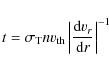
where
Taking the thousands of, mostly weak, UV absorption lines for each
ion into account, CAK estimated the following analytic power-law approximation for M(t)

where
However, as a gas becomes more ionized, either collisionally from an increased temperature, or through photoionization due to the intense UV source, the number of transitions available for absorption is reduced quite dramatically. In launching AGN winds this is a well known problem, and ad hoc schemes to shield the gas have been proposed (e.g. ``hitchhiking gas'', Murray & Chiang 1997).
![\begin{figure}
\par\includegraphics[width=8.5cm,clip]{12579fg1.eps}
\vspace*{4mm}
\end{figure}](/articles/aa/full_html/2010/08/aa12579-09/img23.png)
|
Figure 1:
Analytic approximation for the parameters K (solid line) and
|
| Open with DEXTER | |
A useful, second-order approximation, which takes the ionization
state of the gas into account and solves the divergence of the previous equation for small t, is the following (Abbott 1986)
![\begin{displaymath}M(t) = K \times t^{-\alpha} \times \left[\frac{(1+\tau_{\rm MAX})^{1-\alpha}-1}{\tau_{\rm MAX}^{1-\alpha}}\right]
\end{displaymath}](/articles/aa/full_html/2010/08/aa12579-09/img24.png)
with
![\begin{figure}
\par\includegraphics[width=8.8cm,clip]{12579fg2.eps}
\vspace*{4mm}
\end{figure}](/articles/aa/full_html/2010/08/aa12579-09/img27.png)
|
Figure 2: Force multiplier M(t) vs. optical depth t for a neutral gas in the CAK formulation (straight dashed line), and the Abbott (1982) and Stevens & Kallman (1986) formulation, that allow for ionization state and are more accurate for low effective optical depth (t<10-5). |
| Open with DEXTER | |
Using these results, P00 developed a code which solves the hydrodynamical
equations for a wind arising from an accretion disk, pushed by a central
radiation force described by the above equations. In this work, a SS disk is
assumed, and the ionization state is determined by the incident X-ray radiation
from the central source. The main conclusion of P00 (in agreement with the
previous work of Murray et al. R1995) is that a wind can easily arise from the
accretion disk of AGN, under some initial conditions (SS disk, with a choice of
free parameters such as the Eddington ratio and the X/UV ratio, which will be
discussed in the next Sections). The dependence of the wind properties on the
black hole mass and accretion efficiency is particularly interesting for they
can now be tested against observations, as we discuss below. The black hole
mass,
![]() and the accretion efficiency relative to Eddington,
and the accretion efficiency relative to Eddington,
![]() ,
are the parameters determining the luminosity of AGN.
,
are the parameters determining the luminosity of AGN.
3 Radiation-driven acceleration of a wind
Several physical effects need to be considered in the equations of the
radiation force, to understand whether this external force is capable
of accelerating the wind up to velocities of ![]() 104 km s-1 or higher, as observed in BAL quasars.
104 km s-1 or higher, as observed in BAL quasars.
The results summarized above (Sect. 2) show that a
radiation-driven wind can
arise from accretion disks in AGNs. However, the breadth of initial
conditions
that produce such a wind are at present unknown. First, while the SS
disk is a
plausible solution, many other disk structures are possible. Secondly,
and more importantly, even within the SS disk paradigm the initial
parameters are unknown: the black hole
mass, the Eddington ratio, and the viscosity parameter
![]() .
Finally, since the physical mechanism for the initial launching of a wind is not known,
the radius at which the wind is launched is also unknown. However, recent
studies of warm absorber winds in local AGNs suggest that winds on scales as
small as a few thousand gravitational radii from the central black hole are
possible (Krongold et al. 2006).
.
Finally, since the physical mechanism for the initial launching of a wind is not known,
the radius at which the wind is launched is also unknown. However, recent
studies of warm absorber winds in local AGNs suggest that winds on scales as
small as a few thousand gravitational radii from the central black hole are
possible (Krongold et al. 2006).
An important aspect of the solutions, found in the papers of Murray
et al. (R1995) and P00, is that the sonic and critical points of
the wind are
reached at a low height H above the disk with respect to the distance from
the central source R (H/R<0.1). Also, the velocities at the sonic and
critical points are a few 100 km s-1, which is only a few
percent of the final BAL velocities (![]() 104 km s-1).
104 km s-1).
As discussed briefly in the introduction, radiation pressure is expected to be relevant (and probably dominant) in the wind acceleration, regardless of the details of the launching mechanism. However, following the theory summarized in Sect. 2, in order for the absorption line mechanism to be effective, a balance between the intensity of the X-ray radiation (which determines the ionization parameter) and the intensity of the UV radiation (which provides the momentum needed by the gas to accelerate to high velocities) is required (Murray & Cheng R1995).
In this paper we discuss the general conditions for the acceleration of a
line-driven wind after the launching phase. In particular we investigate
whether the ``thin wind'' geometry proposed by Elvis (2000),
which is successful in explaining a wide set of observational
properties, can arise naturally. The main unexpected features of the
Elvis (2000) geometry are that (1) the wind is thin (![]() /R < 1); and that (2) the wind is initially quasi-vertical, making a hollow cylinder of height
/R < 1); and that (2) the wind is initially quasi-vertical, making a hollow cylinder of height ![]() ,
before becoming a radial, biconical flow.
,
before becoming a radial, biconical flow.
3.1 The QWIND code
We developed the QWIND code with the following assumptions:
- 1.
- The X-ray source is point-like, isotropic and located at the center of the disk.
- 2.
- The UV/optical source is the accretion disk, emitting according to the SS
model, which gives
 .
In our model the wind inner radius can
be as small as 100 RS,
so the dimensions of the UV/optical source is
non-negligible, and the disk cannot be considered a point source.
Therefore,
the dependence of the disk emissivity with radius, and the actual
continuum
emitting disk extent are included. We also take into account the
anisotropy of
the disk emission, which has important consequences for the wind
properties. The radiation is zero on the disk plane, and increases with
the cosine of the
inclination angle of the disk with respect to the wind. Limb darkening
(Fukue & Akizuki 2007), which would accentuate this effect, has
been neglected.
.
In our model the wind inner radius can
be as small as 100 RS,
so the dimensions of the UV/optical source is
non-negligible, and the disk cannot be considered a point source.
Therefore,
the dependence of the disk emissivity with radius, and the actual
continuum
emitting disk extent are included. We also take into account the
anisotropy of
the disk emission, which has important consequences for the wind
properties. The radiation is zero on the disk plane, and increases with
the cosine of the
inclination angle of the disk with respect to the wind. Limb darkening
(Fukue & Akizuki 2007), which would accentuate this effect, has
been neglected.
- 3.
- The gas is launched from the disk at all radii between an inner radius
 and an outer radius
 ,
to a height H above the disk, with given density n, temperature T, and initial vertical velocity v0. The
radial velocity of this newly launched gas is zero, while the angular velocity
in the disk plane is Keplerian.
,
to a height H above the disk, with given density n, temperature T, and initial vertical velocity v0. The
radial velocity of this newly launched gas is zero, while the angular velocity
in the disk plane is Keplerian.
- 4.
- The wind is subject only to the central gravitational force FG due to
the black hole of mass
 and radiation force Fr. Internal gas
pressure is neglected, as is the gravity of the disk.
and radiation force Fr. Internal gas
pressure is neglected, as is the gravity of the disk.
- 5.
- The radiation force in each element of the gas is computed using the CAK
and Abbott (1986) equations described in Sect. 2 (Eqs. (2) and (3)). The
ionization parameter,
 ,
is determined assuming a cross-section
,
is determined assuming a cross-section
 if
if  ,
and
,
and
 if
if
 .
This simple approximation reflects the fact that when the ionization
factor is too high, there are no bound electrons for photoelectric absorption to
be effective. Below this critical value, photoelectric absorption on the
electrons in the inner shells of metals is much more effective than Thomson
scattering in removing X-ray photons. Using this approximation, if ,
X-rays penetrate deep into the wind, keeping
high, until the Thomson
optical depth is higher than 1 (
.
This simple approximation reflects the fact that when the ionization
factor is too high, there are no bound electrons for photoelectric absorption to
be effective. Below this critical value, photoelectric absorption on the
electrons in the inner shells of metals is much more effective than Thomson
scattering in removing X-ray photons. Using this approximation, if ,
X-rays penetrate deep into the wind, keeping
high, until the Thomson
optical depth is higher than 1 (
 cm-2) or the R2factor makes
decrease below 105. Until this point, the radiation force
is negligible because M(t) is small. Deeper inside the wind, where
cm-2) or the R2factor makes
decrease below 105. Until this point, the radiation force
is negligible because M(t) is small. Deeper inside the wind, where
 ,
the UV radiation is also fully absorbed, and again
,
and therefore the radiation force will be negligible in this case too. If instead
the X-rays are absorbed in a thin
layer
,
the UV radiation is also fully absorbed, and again
,
and therefore the radiation force will be negligible in this case too. If instead
the X-rays are absorbed in a thin
layer![[*]](/icons/foot_motif.png)
 cm-2 and the ionization parameter
drops as
cm-2 and the ionization parameter
drops as
 ,
rapidly reaching the values at which the force multiplier becomes significantly higher than 1.
,
rapidly reaching the values at which the force multiplier becomes significantly higher than 1.
|
(4) |
where
Our choice to integrate over the disk structure is motivated by the non-negligible dimensions of the disk with respect to the inner wind streams: in our computation the disk emission is calculated out to a radius of 400 RS(even if the contribution to the total luminosity is negligible for R > 100 RS), while the inner wind radius is 100 RS (see next section for further details on the computation domain).
The computation starts from the innermost stream line (free from absorption), and then proceeds to the outer ones. At each step, the calculations are done in the following order:
- 1.
- We estimate the absorption due to the inner stream lines. For the UV component, this is done simply adding the column densities of the inner stream lines, and multiplying by the Thomson cross-section. For the X-ray component, the computation is more complex: for each stream line crossed by the light ray from the disk element, we estimate the ionization factor and then, depending on its value, the X-ray cross section, following the prescription described above.
- 2.
- Using the absorption correction estimated in the previous point, and integrating over each disk element, we compute the flux on our wind element.
- 3.
- We estimate the density of the gas element from the values of density, mass and velocity of the previous computation step, and requiring mass conservation.
- 4.
- We estimate the force multiplier M(t), following the prescription described in the 5th point of the code properties (above).
- 5.
- We obtain the acceleration on the gas element, and we compute the new spatial coordinates and velocity.
Neglecting the internal gas pressure makes the stream lines of gas in QWIND intersect unphysically. When two stream lines intersect, this means that the gas in the internal line is pushed outwards more than the gas on the external line. In reality this obviously cannot happen, and is prevented by the horizontal component of the gas pressure. However, the two stream lines do delineate a limiting cone that a fully modeled wind must keep within. The gas pressure force between the two ``lines'' will make the gas move along a line whose inclination angle with respect to the disk axis is intermediate between the two lines computed by QWIND. This approximation therefore makes the results of QWIND usable only in this bounding sense, but should not change the general findings of interest, i.e. whether the wind can be accelerated by radiation pressure, the approximate angles to the disk, and covering factor of the central source, since these properties strongly affect the observables.
Another important effect neglected in our treatment is the change in momentum at the bending of the wind, which is expected to produce shocks and, possibly, soft X-ray emission, although this is unlikely to dominate the X-ray luminosity of the AGN. The case for the outflowing gas as a source of the soft X-ray excess observed in many quasars has been discussed by Pounds et al. (2003).
The number of stream lines used in the runs discussed in this paper is kept to just 20. We also made several runs with a larger number of lines (50), to check for discretization effects and found that the properties of the solutions do not change significantly.
The initial density of the wind at a radius R is one of the main free parameters
of our model. In general, we parametrize the density as
![]() .
Two particularly interesting cases
are
.
Two particularly interesting cases
are ![]() (constant density at all radii) and
(constant density at all radii) and
![]() ,
the density
scaling in the SS disk. In this paper, we adopt
,
the density
scaling in the SS disk. In this paper, we adopt ![]() in our examples.
Different cases (and, in particular, the SS disk-like profile, will be
investigated in a forthcoming paper.
in our examples.
Different cases (and, in particular, the SS disk-like profile, will be
investigated in a forthcoming paper.
The initial vertical velocity v0 is a free parameter of the code and is a few 100 km s-1. This velocity is much lower than the escape velocity, therefore most of the kinetic energy needed to make a wind must be provided by the external radiation force.
With these assumptions, the total mass outflowing from the disk is easily derived, integrating the contribution from each disk ring. The fraction of this mass that falls back onto the disk versus the fraction which escapes through a wind, depends on the subsequent acceleration phase, and is studied by our model.
The initial parameters v0 and
![]() are
in reality a result of the
previous launching phase. For example, in a purely radiation-driven
wind, the
mass loss rate is uniquely determined by the regularity and stability
conditions at the ``critical point'' (CAK, Lamers & Cassinelli
1999; Murray et al. R1995). Since we are not studying this
launching phase here, a fundamental requirement
is that our final results do not depend critically on the exact values
of these
parameters. Since the density profile does affect the acceleration
phase of the
wind (because it determines, together with the X-ray flux, the
ionization
parameter), it is particularly important that the final results of the
acceleration phase are independent of the exact value of the initial
velocity,
provided that it is small compared with the final velocity, and large
enough to
be supersonic (this, for temperatures of a few 106 K implies v0 a few 102 km s-1). As we discuss in detail below, we have
carefully checked that this is indeed the case for our wind solutions, and that,
for particular values of the initial velocity (inside the range mentioned
above), our solutions satisfy the critical point conditions for a purely
radiation-driven wind.
are
in reality a result of the
previous launching phase. For example, in a purely radiation-driven
wind, the
mass loss rate is uniquely determined by the regularity and stability
conditions at the ``critical point'' (CAK, Lamers & Cassinelli
1999; Murray et al. R1995). Since we are not studying this
launching phase here, a fundamental requirement
is that our final results do not depend critically on the exact values
of these
parameters. Since the density profile does affect the acceleration
phase of the
wind (because it determines, together with the X-ray flux, the
ionization
parameter), it is particularly important that the final results of the
acceleration phase are independent of the exact value of the initial
velocity,
provided that it is small compared with the final velocity, and large
enough to
be supersonic (this, for temperatures of a few 106 K implies v0 a few 102 km s-1). As we discuss in detail below, we have
carefully checked that this is indeed the case for our wind solutions, and that,
for particular values of the initial velocity (inside the range mentioned
above), our solutions satisfy the critical point conditions for a purely
radiation-driven wind.
We next discuss the solutions obtained with our code QWIND for different choices of initial parameters. First, we concentrate on a particular ``baseline'' solution, in order to understand the physics of the wind. Then, in Sect. 3.3 we discuss the stability of our solutions. In Sect. 3.4 we discuss the dependence of the disk properties on the initial physical conditions. In Sect. 3.5 we briefly discuss a small survey of parameters in order to show the potential of our method in studying the wind properties in a variety of physical conditions.
A systematic analysis of all the variables, including different density profiles, and the effect of toroidal magnetic fields, will be the subject of a forthcoming paper.
3.2 Results: the baseline model, a case study
We show here the results obtained from running QWIND with the initial parameters given in Table 1. The inner and outer radii were chosen in order to investigate the region where a radiation-driven wind is expected, starting from an inner radius close to the outer UV-emitting region of the accretion disk, and studying the solutions up to an outer radius large enough to contain the inner broad line region. The initial velocity was arbitrarily chosen. The important points related to this parameter are: (a) its value must be small compared with the escape velocity; and (b) the exact initial value should not significantly affect the final results.
A further fundamental parameter in the model is the ratio between ionizing
radiation and bolometric emission, fX.
Considering that the whole 0.1-100 keV
spectrum contributes to the gas ionization, and that the wavelength
range of the intrinsic disk emission is from optical to X-rays, a
typical value for this
ratio is
![]() % (e.g. Elvis et al. 1994; Risaliti & Elvis 2004). Quite
different values are however possible, due to the large dispersion of the X-ray
to optical ratio among quasars, and to its dependence on optical luminosity
(e.g. Steffen et al. 2006; Young et al. 2010). We discuss the effects of changing this parameter in the next sections.
% (e.g. Elvis et al. 1994; Risaliti & Elvis 2004). Quite
different values are however possible, due to the large dispersion of the X-ray
to optical ratio among quasars, and to its dependence on optical luminosity
(e.g. Steffen et al. 2006; Young et al. 2010). We discuss the effects of changing this parameter in the next sections.
Table 1: Baseline QWIND model parameters.
![\begin{figure}
\par\includegraphics[width=8.5cm,clip]{12579fg3.eps}
\vspace*{-2mm}\end{figure}](/articles/aa/full_html/2010/08/aa12579-09/img68.png)
|
Figure 3:
Results of the simulations assuming a constant initial density profile. In this example,
|
| Open with DEXTER | |
![\begin{figure}
\par\includegraphics[width=8.5cm,clip]{12579fg4.eps}
\vspace*{-1mm}\end{figure}](/articles/aa/full_html/2010/08/aa12579-09/img69.png)
|
Figure 4: Force multiplier, M(t), (upper plot) and velocity (lower plots) versus radius for the fifth stream line in our case study. The dashed line in the lower plot represents the escape velocity as a function of the distance from the central black hole. See text for details. |
| Open with DEXTER | |
The main properties of the solutions are shown in Fig. 3. In the upper panel we show the wind lines in a plane perpendicular to the accretion disk. In the lower panel we show the ratio between the final velocity and the escape velocity for each wind line. By definition, we have a wind when the gas velocity becomes higher than the escape velocity, i.e. when the ratio in Fig. 3b grows to values greater than 1. In Fig. 4 we show the velocity profile and force multiplier M(t) for the fifth stream line, i.e. the one reaching the highest final velocity.
Several interesting properties of the wind can be drawn from Figs. 3 and 4:
- Initial distance: Fig. 3b shows that the baseline model
gas reaches escape velocity only if it is launched between
 150 RS and
250 RS. At smaller radii, the gas is too ionized for the radiation
force to be effective. At greater radii, the UV radiation is not sufficient to
push the gas up to escape velocity. The exact values for the allowed radius
range depends on the inner radius (in our case
150 RS and
250 RS. At smaller radii, the gas is too ionized for the radiation
force to be effective. At greater radii, the UV radiation is not sufficient to
push the gas up to escape velocity. The exact values for the allowed radius
range depends on the inner radius (in our case
 ). If, for
example,
). If, for
example,
 (and all the other initial parameters are the same), it would be impossible to have a wind at R=300 RS, because the gas is too
ionized, due to the absence of shielding from the central X-ray emission. A wind
at larger radii could however be possible, as we show in Fig. 3. QWIND
modeling thus provides a simple explanation for the existence of a wind arising
only from a narrow range of distances from the center.
(and all the other initial parameters are the same), it would be impossible to have a wind at R=300 RS, because the gas is too
ionized, due to the absence of shielding from the central X-ray emission. A wind
at larger radii could however be possible, as we show in Fig. 3. QWIND
modeling thus provides a simple explanation for the existence of a wind arising
only from a narrow range of distances from the center.
- Inner failed wind: the inner stream lines form a ``failed wind'' that shields the outer stream lines from the central X-ray radiation. This shielding is fundamental to decreasing the ionization parameter in these stream lines, so allowing an effective radiative acceleration. This inner component fulfils the function of the ``hitchhiking gas'' invoked by Murray & Cheng (R1995).
- Radiation force: the upper panel of Fig. 4 shows the
profile of the force multiplier M(t) for the fifth stream line in Fig. 5. Note that the maximum value is never higher than 30. The relatively low
values of M(t) (well below the values >100 estimated by CAK in hot stars)
imply that only fairly large values of M/M
 (>0.03) can produce an escaping wind.
A more technical consequence of the estimated values of M(t) is that the correction factor in Eq. (3) is never important, and Eq. (2) is a good approximation of the force multiplier (Fig. 2, i.e.
 ). This makes possible an analytic analysis of the wind launching problem, which we discuss in Sect. 4.
- Velocity: Fig. 4 (lower panel) shows the velocity profile
for the fifth stream line of our case study. The acceleration is fast, and the
escape velocity is reached at 500 RS. Then the velocity continues to
slightly increase. In this phase the radiation force is still effective in
supporting the wind against gravity. Indeed, the ``effective'' Eddington ratio,
which depends on the actual one,
 ,
the force multiplier, and the inclination angle
,
the force multiplier, and the inclination angle  of the disk as seen from the wind line, is
 up to large radii
(
up to large radii
(
 ).
).
- Geometry: Fig. 3a shows that the gas rises vertically for
50 RS,
and then bends toward a radial direction. Whether the gas falls
down or maintains this direction depends on the effectiveness of the
radiation
force (see below). The angle of the wind above the disk is
approximately 20 deg., giving a substantial covering factor of
35%. We note that the actual
value of the covering angle is somewhat uncertain because the lines are
treated
as independent while, in reality, when two lines intersect, the gas
pressure
from the inner line pushes the gas on the outer line outwards, altering
the
final covering factor.
![\begin{figure}
\par\includegraphics[width=7.8cm,clip]{12579fg5.eps}
\end{figure}](/articles/aa/full_html/2010/08/aa12579-09/img77.png)
|
Figure 5:
Ratio between the gas final velocity and its escape velocity for several values of the Eddington ratio,
|
| Open with DEXTER | |
3.3 Check of initial conditions
In order to test the reliability of our initial conditions, in particular regarding the initial values of the vertical velocity and the height above the disk, we performed two checks:
- 1.
- We varied the initial height from H=5 RS to H=15 RS, and the initial velocity from 100 to 300 km s-1. No significant change in the final properties of the wind was found.
- 2.
- We followed the wind streamlines backward in time down to the critical point (estimating this location as in Murray et al. R1995) and required that our solutions satisfy the regularity and stability conditions at the critical point (CAK). We iteratively varied the initial velocity until a consistent solution was found. A solution was found with a value of the initial velocity within our range of study (v0 = 100-300 km s-1).
3.4 Dependence on the individual parameters
In order to explore the dependence of our solutions on the initial
parameters,
we proceed in two steps: first, we analyze several cases close to the
baseline
model, changing the density, the X-ray to UV ratio, the Eddington
ratio, and the black hole mass, in turn. Then, in the next subsection,
we show the results of a survey of the
![]() space for a few choices of the other initial parameters to show the
potential of our method for exploring the parameter space of initial
conditions.
space for a few choices of the other initial parameters to show the
potential of our method for exploring the parameter space of initial
conditions.
First, starting from the baseline model (Table 1), we
systematically changed
![]() ,
fx, n8,
,
fx, n8,
![]() ,
one at a time: in Figs. 5-8 we show plots analogous to that in
Fig. 3b, i.e. the ratio between the final wind velocity and the escape velocity,
,
one at a time: in Figs. 5-8 we show plots analogous to that in
Fig. 3b, i.e. the ratio between the final wind velocity and the escape velocity,
![]() ,
against the initial wind radius
,
against the initial wind radius![]() . From these results several additional indicators of the physical processes
dominating the wind can be obtained, based on the dependence of
. From these results several additional indicators of the physical processes
dominating the wind can be obtained, based on the dependence of
![]() on
the:
on
the:
- Eddington ratio
(Fig. 5): Too low a
value (panel A,
 implies that the radiation is inadequate
to accelerate the gas to escape velocity. With a higher value (panel B,
implies that the radiation is inadequate
to accelerate the gas to escape velocity. With a higher value (panel B,
 ,
a stream line is able to slightly exceed the escape
velocity, thus forming a wind. Finally, for much higher values (panel C,
,
a stream line is able to slightly exceed the escape
velocity, thus forming a wind. Finally, for much higher values (panel C,
 ,
to be compared with our case study with
,
to be compared with our case study with
 )
a wind is effectively launched, but at larger radii than in the
previous cases. This is due to the higher X-ray luminosity, which
over-ionizes the gas up to larger distances from the center.
)
a wind is effectively launched, but at larger radii than in the
previous cases. This is due to the higher X-ray luminosity, which
over-ionizes the gas up to larger distances from the center.
It is interesting to note that the maximum velocity reached by the wind in the case
is less than in the baseline case of
Fig. 3,
despite the higher Eddington ratio. This is due to the
reduction of the UV radiation pressure on the stream lines with the
``right''
ionization state, due to the higher distance. This result shows in a
simple way that, due to the different dependences of the the physical
conditions of the wind elements on the initial parameters, a higher luminosity does not
automatically imply a faster wind. In our case, the intuitive increase of the
wind velocity is observed increasing the Eddington ratio from 0.2 to 0.5, but
not with the further increase to 0.9.
- Density of the gas, n7 (Fig. 6): At low values of the
density (left plot, n7=3, c.f. n7=20 in the standard case), the gas is
overionized even at large radii, and it is therefore impossible to launch a
wind. Increasing the density (n7=10, right plot) the ionization parameter,
,
decreases, making it easier to push the gas effectively through the
line-absorption driven force. An even higher density shifts the wind towards
inner radii, because the over-ionization region is limited to a smaller region.
![\begin{figure}
\par\includegraphics[width=7.8cm,clip]{12579fg6.eps}
\end{figure}](/articles/aa/full_html/2010/08/aa12579-09/Timg85.png)
Figure 6: Ratio between the gas final velocity and its escape velocity for several values of the initial gas density,
 .
The red dashed line reproduces the same profile for the ``case study'' shown in Fig. 3.
.
The red dashed line reproduces the same profile for the ``case study'' shown in Fig. 3.
Open with DEXTER - The ratio fX between X-ray and disk radiation (Fig. 7):
Too high a value of fX (in our example,
fX = 25%, corresponding to a 2 keV to 2500 Å slope of
 )
produces a higher ionization parameter,
and makes it more difficult to accelerate the gas. Lower values (fX= 5%,
fX= 10%, corresponding to
)
produces a higher ionization parameter,
and makes it more difficult to accelerate the gas. Lower values (fX= 5%,
fX= 10%, corresponding to
 and
and
 ,
respectively) mean a smaller ionizing continuum, and therefore a lower
ionization factor for the inner gas of the wind, which can be accelerated up to
the escape velocity. This effect was first noted by Murray & Chiang (R1995).
,
respectively) mean a smaller ionizing continuum, and therefore a lower
ionization factor for the inner gas of the wind, which can be accelerated up to
the escape velocity. This effect was first noted by Murray & Chiang (R1995).
![\begin{figure}
\par\includegraphics[width=7.8cm,clip]{12579fg7.eps}
\end{figure}](/articles/aa/full_html/2010/08/aa12579-09/Timg89.png)
Figure 7: Ratio between the gas final velocity and its escape velocity for several values of the ratio fX between the X-ray and UV flux. The red dashed line reproduces the same profile for the ``case study'' shown in Fig. 3.
Open with DEXTER ![\begin{figure}
\par\includegraphics[width=7.8cm,clip]{12579fg8.eps}
\end{figure}](/articles/aa/full_html/2010/08/aa12579-09/Timg90.png)
Figure 8: Ratio between the gas final velocity and its escape velocity for several values of the central black hole mass,
.
The red dashed line reproduces the same profile for the ``case study'' shown in Fig. 3.
Open with DEXTER - Black hole mass (Fig. 8): The wind properties strongly
depend on the black hole mass. The dependence is quite complex, since the
different physical parameters (ionization state, UV flux, disk temperature)
scale in different ways with the black hole mass. Varying the black hole mass
and leaving the other parameters as in our case study, we see that the higher
the mass, the closer in is the wind. For the highest mass value
(
 )
no wind is launched with the adopted choice of the
initial parameters. The main physical driver of this behavior is the ionization
parameter,
)
no wind is launched with the adopted choice of the
initial parameters. The main physical driver of this behavior is the ionization
parameter,
 .
Since
.
Since
 (for a fixed
)
and the distance in physical units is
(for a fixed
)
and the distance in physical units is
 (for a fixed value in units of RS), the ionization parameter at a given distance in units of RS decreases with
.
The distance (in units of RS)
at which we have the ``right'', wind-producing, balance between
ionization state and UV irradiation therefore decreases with increasing
black hole mass, reaching values lower than our inner radius for
.
In this case, it may be possible to obtain a wind from
radii
(for a fixed value in units of RS), the ionization parameter at a given distance in units of RS decreases with
.
The distance (in units of RS)
at which we have the ``right'', wind-producing, balance between
ionization state and UV irradiation therefore decreases with increasing
black hole mass, reaching values lower than our inner radius for
.
In this case, it may be possible to obtain a wind from
radii
 .
This scenario will be studied in a broader analysis of the
parameter space, which will be presented in a forthcoming paper. Here we only
note that this result does not imply that a wind is impossible at high masses:
an example of wind from a 10
.
This scenario will be studied in a broader analysis of the
parameter space, which will be presented in a forthcoming paper. Here we only
note that this result does not imply that a wind is impossible at high masses:
an example of wind from a 10
 black hole is presented in the next section, where we show that a different choice of the initial density leads
to higher ionization parameters, shifting the ``wind zone'' towards higher
radii. In particular, we show that an initial value of the density N7 =1(i.e. 20 times lower than our baseline case) implies that a wind can be
launched only with black hole masses on the order of 10
.
black hole is presented in the next section, where we show that a different choice of the initial density leads
to higher ionization parameters, shifting the ``wind zone'' towards higher
radii. In particular, we show that an initial value of the density N7 =1(i.e. 20 times lower than our baseline case) implies that a wind can be
launched only with black hole masses on the order of 10
.
3.5 Parameter survey
In order to test the ability of QWIND to perform complete surveys of the
parameter space, we ran a grid of
![]() models,
adopting the parameters of our baseline study, and varying the black
hole mass and the Eddington ratio in the range 107-10
models,
adopting the parameters of our baseline study, and varying the black
hole mass and the Eddington ratio in the range 107-10
![]() and 0.1-1, respectively. The result is shown in Fig. 9. The allowed region for the wind launching extends down to
and 0.1-1, respectively. The result is shown in Fig. 9. The allowed region for the wind launching extends down to
![]() ,
showing that a radiation-driven wind is possible at
luminosities much below the Eddington limit (as was also shown, in more detail,
for a single case in Fig. 5b). Clearly, in these cases the enhancement
of the radiation force due to line absorption plays a fundamental role.
,
showing that a radiation-driven wind is possible at
luminosities much below the Eddington limit (as was also shown, in more detail,
for a single case in Fig. 5b). Clearly, in these cases the enhancement
of the radiation force due to line absorption plays a fundamental role.
![\begin{figure}
\par\includegraphics[width=8.0cm,clip]{12579fg9.eps}
\end{figure}](/articles/aa/full_html/2010/08/aa12579-09/img99.png)
|
Figure 9:
Results of a survey of the
|
| Open with DEXTER | |
As a further example of the application of QWIND we also tested the
scenario of a hot, low density wind with a less substantial mass outflow. To
test this, we run a QWIND grid analogous to the one described above, but
with an initial density 20 times lower (
![]() cm-3). The results
are shown in Fig. 10. In general, too low a density implies a too
high ionization, and the wind cannot be launched. The situation is different
only at very high masses, where the distances from the central source are large
enough to provide the requested balance between ionization parameter and
intensity of the UV source.
cm-3). The results
are shown in Fig. 10. In general, too low a density implies a too
high ionization, and the wind cannot be launched. The situation is different
only at very high masses, where the distances from the central source are large
enough to provide the requested balance between ionization parameter and
intensity of the UV source.
![\begin{figure}
\par\includegraphics[width=8.0cm,clip]{12579fg10.eps}
\end{figure}](/articles/aa/full_html/2010/08/aa12579-09/img100.png)
|
Figure 10:
Results of a survey of the
|
| Open with DEXTER | |
4 Analytic approximations
Since our main aim is to understand which physical conditions allow wind acceleration, we can search for further simplifications which allow an even simpler treatment, based on an analytic model. Our aim here is not to study the details of the wind solutions, but rather to explore the parameter space in order to understand which are the initial conditions required in order to have accelerations up to several thousand km s-1. The analytic treatment lets us search for the existence of wind solutions by finding regions of parameter space that satisfy two conditions: (1) that the final velocity exceeds the escape velocity; and (2) that the gas must not be overionized.
In this section we will make three extra approximations to the dynamical equations of the wind, which allow the equation of motion to be integrated analytically, so that the final velocity can be calculated directly. The approximations are:
- 1.
- An energy source with a constant inclination with respect to the wind. For the X-rays, this is the same as assumed in QWIND (spherically symmetric emission). For the UV, this is equivalent to the assumption of a fixed inclination angle of the wind stream lines.
- 2.
- Neglect of the gravitational term in the dynamic equation as, once the line-driven acceleration mechanism becomes effective, it usually dominates the gravitational term by a factor of 10 or more (see Sect. 4.3).
- 3.
- Line driving is well-reproduced by the simple equation
 ,
which is valid only when the wind is not overionized, but we
require a low ionization parameter as a condition for the acceleration of the
wind (see below).
,
which is valid only when the wind is not overionized, but we
require a low ionization parameter as a condition for the acceleration of the
wind (see below).
We discuss the third assumption in the next subsection. The integration of the equation of motion, and the condition on the final velocity are discussed in Sect. 4.2. We then show the results for a limited set of initial parameters, and, finally, we compare our results with those obtained with QWIND.
4.1 Relation between M(t) and 
Here we show that the equation of the force multiplier, M(t) can be simplified
into two regimes, depending on the ionization factor:
![]() .
We then discuss the equation describing
the motion of a gas element inside the wind.
.
We then discuss the equation describing
the motion of a gas element inside the wind.
In order to estimate the range of values of t for which the correction factor
of M(t) becomes important, and therefore M(t) saturates to its asymptotic
limit, we expand Eq. (3) for small t, obtaining
This shows that in order to have

|
(6) |
From Fig. 1 , for
If ![]() the situation is completely different, since it is obvious from
Fig. 1 that the line absorption becomes negligible compared with
electron scattering, and in this condition no wind can be launched unless the
luminosity is super-Eddington. This is why the wind models of Murray & Chiang
(1997) require additional, ``hitchhiking'' gas, to shield the gas that was to be accelerated, reducing
the situation is completely different, since it is obvious from
Fig. 1 that the line absorption becomes negligible compared with
electron scattering, and in this condition no wind can be launched unless the
luminosity is super-Eddington. This is why the wind models of Murray & Chiang
(1997) require additional, ``hitchhiking'' gas, to shield the gas that was to be accelerated, reducing ![]() .
Therefore, in the following we shall assume
.
Therefore, in the following we shall assume
![]() in studying the dependence of the wind from the other parameters.
Now let us consider a gas element in the outflow at radial distance R from the
center. The gas element is subject to gravitational force,
in studying the dependence of the wind from the other parameters.
Now let us consider a gas element in the outflow at radial distance R from the
center. The gas element is subject to gravitational force,
![]() ,
and to the radiation force,
,
and to the radiation force,
![]() .
The force multiplier M(t) is given by Eq. (3), and depends on the density
profile of the gas making up the wind. We assume a profile
.
The force multiplier M(t) is given by Eq. (3), and depends on the density
profile of the gas making up the wind. We assume a profile
![]() ,
as in our numeric code.
,
as in our numeric code.
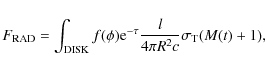
The flux at a given gas element inside the wind is given by
![]() ,
where L0 is the intrinsic disk luminosity, F is the
geometrical factor due the disk inclination (which is assumed to be constant in
this analytical treatment) and A(R)
takes into account the absorption between
the gas element under consideration and the luminosity source. While a
detailed treatment of the absorption term would require a complete
solution of
hydrodynamical and radiative transfer equations, we can make some
useful
approximations:
,
where L0 is the intrinsic disk luminosity, F is the
geometrical factor due the disk inclination (which is assumed to be constant in
this analytical treatment) and A(R)
takes into account the absorption between
the gas element under consideration and the luminosity source. While a
detailed treatment of the absorption term would require a complete
solution of
hydrodynamical and radiative transfer equations, we can make some
useful
approximations:
- That the inner part of the gas is able to reach high enough above the disk that it shields the gas farther out. This assumption is supported by the results of QWIND (Sect. 3), and has the same effect as the assumption of hitchhiking gas by Murray & Chiang (R1995).
- That each ring of gas with thickness
 contributes to radiation
absorption with a column density of
contributes to radiation
absorption with a column density of  .
This is obviously a lower limit, since the wind is not perpendicular to
the central radiation. However, the correction is small and can be
neglected.
.
This is obviously a lower limit, since the wind is not perpendicular to
the central radiation. However, the correction is small and can be
neglected.
|
(7) |
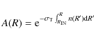
where
![\begin{displaymath}A(R)={\rm e}^{-\frac{0.02}{\beta-1}~n_8~R_{100} M_7\left[1-\left(\frac{R}{R_{\rm IN}}\right)^{1-\beta}\right]}\cdot
\end{displaymath}](/articles/aa/full_html/2010/08/aa12579-09/img117.png)
We can now write the equation of motion for the gas, simply requiring that the force on a gas element is equal to the difference between the external radiation force and the gravitational force. As in the QWIND code (Sect. 3), we neglect the internal pressure term, since we want to discuss the motion of the ion in the supersonic part of the wind, where gas pressure cannot affect the dynamics significantly. Furthermore, we assume that only radial forces are present. This implies the conservation of angular momentum, and a decoupling of the radial and tangential equations. The radial equation of motion can then be written, putting
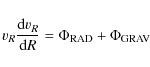
|
(9) |
where the lefthand side gives the radial acceleration, while the righthand side is made up of two terms:
- 1.
- The line-enhanced radiation force, given by the flux multiplied by the
force multiplier M(t), and by a geometrical factor,
 ,
dependent on
the inclination angle
,
dependent on
the inclination angle  of the disk with respect to the gas element
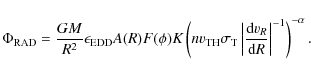
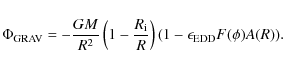
(10) - 2.
- The gravitational force, corrected by a factor
 ,
obtained from angular momentum conservation, assuming that the gas
element moves with the Keplerian velocity at the initial radius
,
obtained from angular momentum conservation, assuming that the gas
element moves with the Keplerian velocity at the initial radius  ,
and decreased by the continuum radiation force, due to Thomson scattering):
,
and decreased by the continuum radiation force, due to Thomson scattering):
In general, Eq. (11) can only be solved using numerical codes.
However, in our case we are interested in some special situations. In
particular, the wind solution we are seeking is characterized by a sudden and
strong radial acceleration (as demonstrated by the results of QWIND shown
in Sect. 3), which changes the gas motion from slow and quasi-vertical to
radial and fast (with velocity higher than the escape velocity). We can assume
that in this accelerating phase the external force is dominant with respect to
the gravitational term, which can be neglected. We also require that the final
wind velocity, vF, exceeds the escape velocity,
![]() ,
within a distance from the center of a few 103 RS. We will then check
whether our solutions fulfill the conditions described above. This consistency
check will only show whether our wind solutions are acceptable, but allows that
other solutions are possible. For example, we expect that, for a large set
of initial conditions, the gas, after initially rising, will fall back onto the
disk. (In these cases the gravitational term is obviously not negligible).
,
within a distance from the center of a few 103 RS. We will then check
whether our solutions fulfill the conditions described above. This consistency
check will only show whether our wind solutions are acceptable, but allows that
other solutions are possible. For example, we expect that, for a large set
of initial conditions, the gas, after initially rising, will fall back onto the
disk. (In these cases the gravitational term is obviously not negligible).
Neglecting the gravitational term, and requiring mass conservation, we obtain
![\begin{displaymath}
R^2v_R\frac{{\rm d}v_R}{{\rm d}R}=\eta\left[R^2v_R\frac{{\rm d}v_R}{{\rm d}R}\right]^\alpha
\end{displaymath}](/articles/aa/full_html/2010/08/aa12579-09/img125.png)
where
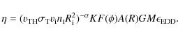
|
(13) |
Since we are studying solutions with rapid radial accelerations, which quickly make the gas motion radial, we can assume that the geometrical factor is constant (
![\begin{displaymath}\eta^{\frac{1}{1-\alpha}}r_{\rm i}^{-1}\left[1-\frac{R_{\rm i}}{R_F}\right] > GMR_F^{-1}\cdot
\end{displaymath}](/articles/aa/full_html/2010/08/aa12579-09/img130.png)
|
(14) |
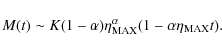
Finally, we adopt the initial density profile discussed above, and we assume
We can then rewrite the above equation as:
![\begin{displaymath}\left[v_{\rm TH}\sigma_{\rm T} v_I n_I R_{\rm i}^2 (GM)^{-1})\right]^{-\alpha} k F_0 A \epsilon{\rm EDD} > 1.
\end{displaymath}](/articles/aa/full_html/2010/08/aa12579-09/img134.png)
|
(15) |
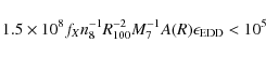
Finally, adopting a proper parametrization for the physical quantities and substituting the numerical values for the constants, and assuming
![\begin{displaymath}
\epsilon_{\rm EDD}>1.1\times10^{-3}
A^{-1}F_0^{-1}\left[\sqrt{T_7}v_7n_8R_{{\rm i},100}^2M_7^{-1}\right]^{0.6}.
\end{displaymath}](/articles/aa/full_html/2010/08/aa12579-09/img135.png)
This condition, when combined with the requirement that the gas not be over-ionized (Sect. 4.2), will allow us to put on the wind-like solutions in a black hole mass - Eddington ratio plane, as we show in Sect. 4.3.
4.2 Effects of X-ray absorption
If the inner part of the wind is too close to the X-ray source, an
over-ionization problem arises. An approximate treatment can be obtained by
considering the X-ray cross-section of the wind gas as in P00. Using the
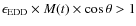
approximation described in Sect. 3, a fundamental requirement for a
radiation-driven wind to be launched is that
![]() ,
where L is the ionizing radiation. Adopting the same parametrizations as in the
previous subsection, the above condition can be written as
,
where L is the ionizing radiation. Adopting the same parametrizations as in the
previous subsection, the above condition can be written as
where A(R) is the unabsorbed fraction of the X-ray radiation, and is given by Eq. (8), the cross-section being the same (for
In our case, the typical intrinsic X-ray spectrum of an AGN is
dominated by soft emission in the 0.1-1 keV band, which gives a
significant - if not dominant -
contribution to the ionization parameter. Therefore, we calculate the
ionization parameter using the luminosity above 0.1 keV. As a
standard value we
assume that of Elvis et al. (1994), where the 0.1-100 keV luminosity is
![]() 15% of the total (i.e. optical-UV-X-ray) emission of an AGN.
15% of the total (i.e. optical-UV-X-ray) emission of an AGN.
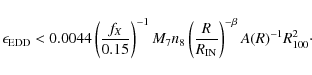
Assuming the density profile of the SS disk
![]() Eq. (17) can be finally
rewritten as
Eq. (17) can be finally
rewritten as
4.3 Analytical results
The constraints from Eqs. (16) and (18) delimit the
region of the black hole mass, Eddington ratio (
![]() )
parameter space in which an outflowing wind can arise.
)
parameter space in which an outflowing wind can arise.
We can use Eqs. (16) and (18) to plot the allowed
wind-launching regions in the
![]() plane. Since
Eq. (18) depends on the initial radius of each streamline, for a
given set of initial parameters (wind inner radius
plane. Since
Eq. (18) depends on the initial radius of each streamline, for a
given set of initial parameters (wind inner radius
![]() ,
density at the
inner radius
,
density at the
inner radius
![]() ,
gas temperature T and X-ray to optical/UV ratio fX)
we compute the allowed region for each single streamline, and then we plot the
convolution of all these regions. In this way, the meaning of the ``analytic
parameter surveys'' are analogous to those plotted in Figs. 9
and 10.
,
gas temperature T and X-ray to optical/UV ratio fX)
we compute the allowed region for each single streamline, and then we plot the
convolution of all these regions. In this way, the meaning of the ``analytic
parameter surveys'' are analogous to those plotted in Figs. 9
and 10.
We assume a baseline set of initial parameters (Table 1), as used
in Eqs. (16) and (18): fX=15%,
![]() K,
K,
![]() cm-3 at
cm-3 at
![]() .
These parameter values are those
required for the gas responsible for the observed UV and X-ray ``Warm absorber''
absorption lines (Nicastro et al. 1999; Netzer et al. 2002; Krongold et al. 2003) in quasar spectra. They are also the physical conditions needed for a
gas confining the BEL clouds (which have
.
These parameter values are those
required for the gas responsible for the observed UV and X-ray ``Warm absorber''
absorption lines (Nicastro et al. 1999; Netzer et al. 2002; Krongold et al. 2003) in quasar spectra. They are also the physical conditions needed for a
gas confining the BEL clouds (which have
![]() cm-3 and
cm-3 and
![]() K, Osterbrock 1989) as noted by Turner et al. (1994) and Elvis (2000).
K, Osterbrock 1989) as noted by Turner et al. (1994) and Elvis (2000).
![\begin{figure}
\par\includegraphics[width=8.5cm,clip]{12579fg11.eps}\vspace*{-1mm}
\vspace*{-2mm}\end{figure}](/articles/aa/full_html/2010/08/aa12579-09/img144.png)
|
Figure 11: Results of our numerical analysis for our baseline set of parameters. The green (shaded) region indicates where a wind can be launched. The analytic estimate is compared with the numerical result obtained with a QWIND survey. |
| Open with DEXTER | |
![\begin{figure}
\par {\includegraphics[width=16cm]{12579fg12.eps} }\end{figure}](/articles/aa/full_html/2010/08/aa12579-09/img145.png)
|
Figure 12:
Results of our numerical analysis for several choices of the initial parameters. The red lines show the total luminosity of the
source. The green (shaded) regions are those allowed for wind launching. Upper left panel: BELR case; upper right panel: hot wind case; lower left panel: wind from an X-ray quiet source; lower right panel: wind with a large inner radius (
|
| Open with DEXTER | |
Figure 11 shows the allowed (
![]() )
parameter
space for the baseline parameters, superimposed to the results of QWIND
for the same set of parameters (already shown in Fig. 9. The two
interesting results emerging from this plot are:
)
parameter
space for the baseline parameters, superimposed to the results of QWIND
for the same set of parameters (already shown in Fig. 9. The two
interesting results emerging from this plot are:
- (1)
- The allowed region based on our analytic approximation is larger than obtained with the more detailed approach based on QWIND. This confirms that our approximations do not miss any possible wind solution, in agreement with our expectations (Sect. 4.1).
- (2)
- The results of the analytic approximations are useful to exclude a significant part of the parameter space where a wind cannot exist. This approach can then be used for a genaral exploration of the parameter space, leaving the more time-consuming numerical approach for a smaller set of parameters. This was not obvious a priori, since too strong an approximation could have led to an too large (and therefore useless) allowed region.
We show in Fig. 12 the allowed regions in four cases, obtained from the baseline case changing one or two initial parameters, in order to test four different physical situations:
- (a) BELR wind: It is interesting to investigate whether BEL gas could be
accelerated directly by the radiation force. Figure 12a shows that
BEL gas cannot be accelerated to high velocities by the radiation force, except
at relatively low mass black holes (M7 < 10) and high Eddington ratios
(except at the lowest masses). The physical reason is that in an overly dense
gas the Doppler shift due to the radial acceleration is insufficient move the
transition to fresh UV continuum, so the gas becomes self-shielded against line
absorption. Thus in a too dense gas the effective optical depth, t, is never
small enough to make the force multiplier M(t) much higher than 1, for
reasonable values of the radial velocity gradient
(
 s-1).
s-1).
We stress that this result does not imply that a wind containing a cold and dense phase is possible only at low masses. Indeed, if the BEL gas is confined by a hot wind, it is expected that the pressure of the warm gas would drive them to similar velocities. However, a more detailed study is needed to test this statement. Here we note only that, in a wind like the one described in Elvis (2000), most of the kinetic energy is in the warm phase (80-90%). Therefore, from an energetic point of view it is likely that the dynamics of the whole wind (comprised of the cold phase, i.e. the BEL gas, and the warm phase) is determined by the warm phase.
- (b) Hot wind: Fig. 12b
shows the allowed region for a hot, low density wind. Only at the
highest masses can such a wind be launched, because of the
over-ionization due the low wind density. The ionization parameter of
the
wind decreases at high BH masses because in our scheme the distance of
the
stream lines is always the same in units of RS. Therefore, increasing the BH
mass implies a linear increase of the luminosity (at a given
)
and a quadratic increase of the physical distance, resulting in a linear
decrease of the ionization parameter with
.
We note that this case is the same as in the second QWIND survey (Fig. 10). Again, the allowed region obtained with the analytic approach is larger than that predicted with QWIND (Fig. 10).
- (c) X-ray weak source: The fraction of the bolometric luminosity emitted
in the X-rays, fX, is important in the determination of the allowed region
for a wind. The value used in the standard parameters set,
fX = 15%,
agrees with the observed spectral energy distributions (SEDs) of PG quasars
(Elvis et al. 1994; Laor et al. 1997). However fX depends on luminosity (Zamorani et al. 1981; Yuan et al. 1998; Steffen et al. 2006; Young et al.
2010) and values of 20-25%
are found in nearby Seyfert galaxies. High values are also found in
radio-loud quasars; in this case however beaming likely plays a role.
On the other side, lower values of 5% are found in high luminosity (
 erg s-1 Hz-1, Yuan et al. 1998) and high redshift (z > 4, Vignali et al. 2002; Steffen et al. 2006) quasars. In Fig. 12c we show the case for an X-ray-quiet source, with fX=5%
and the other parameters as in the baseline study. The allowed region is
increased, because lower X-ray emission implies a lower ionization parameter.
This is important especially at low BH masses, where the requirements to avoid
gas over-ionization are more stringent.
erg s-1 Hz-1, Yuan et al. 1998) and high redshift (z > 4, Vignali et al. 2002; Steffen et al. 2006) quasars. In Fig. 12c we show the case for an X-ray-quiet source, with fX=5%
and the other parameters as in the baseline study. The allowed region is
increased, because lower X-ray emission implies a lower ionization parameter.
This is important especially at low BH masses, where the requirements to avoid
gas over-ionization are more stringent.
- (d) Wind inner radius: We changed the inner wind radius from 100 RS to 300 RS (Fig. 12d). The allowed wind region is smaller than in our baseline study, because part of the parameter space is excluded both at high BH masses (as is apparent from a comparison with Fig. 11), where a wind cannot be launched because the physical distance of the gas is too large for the radiation pressure to be effective.
The analytical results presented here have several important limitations, as
noted at the start of Sect. 4. In addition, our treatment is based on a
condition of existence for the solutions of the equation of motion of a wind
element. This is a less stringent condition than requiring an actual wind
solution for a given set of initial parameters. As a result, real wind
solutions are possible only for smaller parameter regions than those shown in
Figs. 11 and 12. Importantly though, no real solution
outside these regions should exist. The exception is for
![]() ,
for which a wind can be accelerated through electron scattering alone.
,
for which a wind can be accelerated through electron scattering alone.
5 Comparison with previous results
A comparison of our results with those obtained with more complex hydrodynamical codes is useful to test the reliability of QWIND. In particular, we refer to the work of P00, in which a radiation-driven wind from a SS disk is studied, solving the wind equations through a 2-dimensional hydrodynamical code.
The properties of the solutions are remarkably similar. In particular:
- The velocity profile in P00 (their Fig. 2) is remarkably similar, after the wind has bent towards the radial direction. In particular, when the external force becomes effective, and the gas changes its direction, the velocity very rapidly increases up to its maximum value (around 104 km s-1). This agrees with our main approximation, i.e. the separation between a internal pressure-dominated phase and an external radiation-force-dominated phase.
- The ionization parameter profiles are quite similar. This is not
surprising, and indeed is only a check of self-consistency, since we have
adopted the same assumptions for the X-ray cross-section as P00. As discussed
above, in this scenario the ionization parameters rapidly drops from large
(>105) to very low (<103) values across a thin layer of
cm-2.
- The final values for the ejected mass are comparable. We find for our
``case study'' a value of
 yr-1, which is close to that of P00 for the same black hole mass. (Note that the mass loss rate scales as
 ).
).
6 Conclusions, and future work
We have shown that a radiation-driven wind can be accelerated to velocities of about 104 km s-1 from a Shakura-Sunyaev accretion disk at a distance from the central black hole close to that of the BEL clouds, for densities and temperatures in the range observed in quasar warm absorbers.
Thanks to our simple approach, we were able to make an analytic estimate of the parameter space in which a wind solution is allowed, and to build a fast code, QWIND, which can be used to better investigate the dependence on the several unknown initial parameters.
The main limitation of our study is the assumption of a substantial initial velocity (a few 100 km s-1) which makes the wind supersonic from the beginning. We did not discuss the physical mechanism through which the disk provides the initial kinetic energy to the gas.
Our main results are:
- 1.
- Our model reproduces the global results of more complex hydrodynamical codes. This makes us confident that our approach can be used to explore the potentially huge space of initial conditions, in order to understand in which cases a wind can be launched. The results of our analytical study agree with those of the numerical code QWIND, in the sense that the parameters space regions excluded by the analytical analysis are also excluded with the more precise numerical approach.
- 2.
- For initial parameters typical of AGN warm absorbers, a wind can arise
only for relatively high accretion efficiencies (
 )
and in a
narrow range of disk radii. This is due to overionization at smaller
radii, and to a too small a UV radiation field and initial velocity at larger
radii, and is an inherent feature of radiation driven disk winds in AGNs.
)
and in a
narrow range of disk radii. This is due to overionization at smaller
radii, and to a too small a UV radiation field and initial velocity at larger
radii, and is an inherent feature of radiation driven disk winds in AGNs.
- 3.
- The inner part of the gas, which is too overionized to be effectively accelerated, forms a ``failed wind'' which removes the X-ray radiation from directions close to the disk plane, allowing a fast decrease of the ionization parameter with the distance form the central source, and so allowing the line driven wind acceleration at larger radii. This component fulfills the function of the ``hitchhiking gas'' postulated by Murray & Chiang (R1995).
- 4.
- We have shown how QWIND can be used to gain a simple physical understanding of the dependence of the wind properties on the initial parameters, such as the X-ray to UV ratio, the Eddington ratio, the initial density and temperature, the central black hole mass. Some of the results are at first counter-intuitive, as, for example, the non-monotonic dependence of the wind final velocity on the Eddington ratio: in some cases more luminous sources can have slower winds, with the other physical parameters being held constant.
- 5.
- The terminal velocity of the wind is typically
 km s-1, and the cone covering factor is a few percent of the lines of sight. This is in reasonable agreement with observations of BAL
quasars.
km s-1, and the cone covering factor is a few percent of the lines of sight. This is in reasonable agreement with observations of BAL
quasars.
- 6.
- The wind angle above the disk is substantial (20 deg), and so is
neither equatorial nor polar. Some 35% of the viewing directions will see the X-ray and UV continuum source through the wind.
Our main aims at this stage were to check the reliability of our approach, and to give significant examples of its use. The next major step, which will be presented in a forthcoming paper, is a systematic survey of initial parameters, to give a more general view of the physical conditions needed to accelerate winds by line driving. In particular, we will investigate how the results are affected by changes in the wind inner radius and in the initial density and velocity profiles.
AcknowledgementsWe are grateful to Jonathan Mc Dowell for his help with the numerical code, and to the anonymous referee for his/her comments and a close reading of the text, which greatly improved the clarity of the work. This work has been partially supported by NASA grants NNX08AX78G, NNX07AI22G and GO7-8136A, and by grant ASI-INAF I/088/06/0.
References
- Abbott, D. C. 1982, ApJ, 259, 282 [NASA ADS] [CrossRef] [Google Scholar]
- Arav, N., de Kool, M., Korista, K. T., et al. 2001, ApJ, 561, 118 [NASA ADS] [CrossRef] [Google Scholar]
- Antonucci, R. 1993, ARA&A, 31, 473 [Google Scholar]
- Baldwin, J. A. 1977, ApJ, 214, 679 [NASA ADS] [CrossRef] [Google Scholar]
- Bechtold, J., Siemiginowska, A., Shields, J., et al. 2003, ApJ, 588, 119 [NASA ADS] [CrossRef] [Google Scholar]
- Blandford, R. D., & Payne, D. G. 1982, MNRAS, 199, 883 [NASA ADS] [CrossRef] [Google Scholar]
- Brotherton, M. S. 1996, ApJS, 102, 1 [NASA ADS] [CrossRef] [Google Scholar]
- Castor, J. I., Abbott, D. C., & Klein, R. I. 1975, ApJ, 195, 157 [NASA ADS] [CrossRef] [Google Scholar]
- Crenshaw, D. M., Kraemer, S. B., Boggess, A., et al. 1999, ApJ, 516, 750 [NASA ADS] [CrossRef] [Google Scholar]
- Dorodnitsyn, A., Kallman, T., & Proga, D. 2008, ApJ, 687, 97 [NASA ADS] [CrossRef] [Google Scholar]
- Elvis, M., et al. 1994, ApJS, 94, 1 [NASA ADS] [CrossRef] [Google Scholar]
- Elvis, M. 2000, ApJ, 545, 63 [NASA ADS] [CrossRef] [Google Scholar]
- Everett, J. E., & Murray, N. 2007, ApJ, 656, 93 [NASA ADS] [CrossRef] [Google Scholar]
- Fukue, J., & Akizuki, C. 2006, PASJ, 58, 1039 [NASA ADS] [Google Scholar]
- George, I. M., Turner, T. J., Mushotzky, R. et al. 1998, ApJS, 114, 73 [NASA ADS] [CrossRef] [Google Scholar]
- Hamann, F., Korista, K. T., & Morris, S. L. 1993, ApJ, 415, 541 [NASA ADS] [CrossRef] [Google Scholar]
- Hawley, J. F., & Krolik, J. H. 2006, ApJ, 641, 103 [NASA ADS] [CrossRef] [Google Scholar]
- Icke, V. 1980, AJ, 85, 329 [NASA ADS] [CrossRef] [Google Scholar]
- Konigl, A., & Kartje, J. F. 1994, ApJ, 434, 446 [NASA ADS] [CrossRef] [Google Scholar]
- Krongold, Y., Nicastro, F., Brickhouse, N. S., et al. 2003, ApJ, 597, 832 [NASA ADS] [CrossRef] [Google Scholar]
- Kurosawa, R., & Proga, D. 2009, MNRAS, 397, 1791 [NASA ADS] [CrossRef] [Google Scholar]
- Laor, A., Fiore, F., Elvis, M., Wilkes, B. J., & McDowell, J. C. 1997, ApJ, 477, L93 [NASA ADS] [CrossRef] [Google Scholar]
- Lee, L. W., & Turnshek, D. A. 1995, ApJ, 453, L61 [NASA ADS] [CrossRef] [Google Scholar]
- Maloney, P. R., Hollenbach, D. J., & Tielens, A. G. G. M. 1996, ApJ, 432, 606 [Google Scholar]
- Mathur, S., Elvis, M., & Wilkes, B. 1995, ApJ, 452, 230 [NASA ADS] [CrossRef] [Google Scholar]
- Maiolino, R., Salvati, M., Marconi, A., et al. 2001, A&A, 375, 25 [Google Scholar]
- McDowell, J. C., Canizares, C., Elvis, M., et al. 1995, ApJ, 450, 585 [NASA ADS] [CrossRef] [Google Scholar]
- Mineshige, S., & Shields, G. A. 1990, ApJ, 351, 47 [NASA ADS] [CrossRef] [Google Scholar]
- Murray, N., & Chiang, J. 1997, ApJ, 474, 91 [NASA ADS] [CrossRef] [Google Scholar]
- Nicastro, F., Fiore, F., Perola, G. C., et al. 1999, ApJ, 512, 184 [NASA ADS] [CrossRef] [Google Scholar]
- Netzer, H., Chelouche, D., George, I. M. 2002, ApJ, 571, 256 [NASA ADS] [CrossRef] [Google Scholar]
- Ogle, P. M., Cohen, M. H., Miller, J. S., et al. 1999, ApJS, 125, 1 [NASA ADS] [CrossRef] [Google Scholar]
- Ohsuga, K., Mori, M., Nakamoto, T., et al. 2005, ApJ, 628, 368 [NASA ADS] [CrossRef] [Google Scholar]
- Ohsuga, K., Mineshige, S., Mori, M., & Kato, Y. 2009, PASJ, 61, L7 [NASA ADS] [Google Scholar]
- Osmer, P. S., & Shields, J. C. 1999, in Quasars and Cosmology (San Francisco: ASP), ASP Conf. Ser. 162, 235 [Google Scholar]
- Panessa, F., & Bassani, L. 2002, A&A, 394, 435 [NASA ADS] [CrossRef] [EDP Sciences] [Google Scholar]
- Pounds, K. A., Reeves, J. N., King, A. R., et al. 2003, MNRAS, 345, 705 [NASA ADS] [CrossRef] [Google Scholar]
- Proga, D. 2003, ApJ, 585, 406 [NASA ADS] [CrossRef] [Google Scholar]
- Proga, D., & Kallman, T. R. 2004, ApJ, 616, 688 [Google Scholar]
- Proga, D., Stone, J. M., & Drew, J. E. 1998, MNRAS, 295, 595 [NASA ADS] [CrossRef] [Google Scholar]
- Proga, D., Stone, J. M., & Kallman, T. R. 2000, ApJ, 543, 686 [NASA ADS] [CrossRef] [Google Scholar]
- Reynolds, C. S. 1997, MNRAS, 286, 513 [NASA ADS] [CrossRef] [Google Scholar]
- Risaliti, G., Elvis, M., & Nicastro, F. 2002, ApJ, 571, 234 [NASA ADS] [CrossRef] [Google Scholar]
- Risaliti, G., & Elvis, M. 2004, Supermassive Black Holes in the Distant Universe, 308, 187 [Google Scholar]
- Rokaki, E., Lawrence, A., Economou, F., et al. 2003, MNRAS, 340, 1298 [NASA ADS] [CrossRef] [Google Scholar]
- Rudge, C. M., & Raine, D. J. 1998, MNRAS, 297, L1 [NASA ADS] [CrossRef] [Google Scholar]
- Shakura, N. I., & Sunyaev, R. A. 1973, A&A, 24, 337 [NASA ADS] [Google Scholar]
- Schurch, N. J., & Done, C. 2007, MNRAS, 381, 1413 [Google Scholar]
- Siemiginowska, A., Czerny, B., & Kostyunin, V. 1996, ApJ, 458, 491 [NASA ADS] [CrossRef] [Google Scholar]
- Smith, P. S., Schmidt, G. D., Hines, D. C., et al. 2003, ApJ, 593, 676 [NASA ADS] [CrossRef] [Google Scholar]
- Stone, J., & Norman, M. 1992, ApJS, 80, 753 [Google Scholar]
- Stevens, I. R., & Kallman, T. R. 1990, ApJ, 436, 599 [Google Scholar]
- Tajima, Y., & Fukue, J. 1996, PASJ, 48, 529 [NASA ADS] [Google Scholar]
- Vignali, C., Brandt, W. N., Schneider, D. P., Garmire, G. P., & Kaspi, S. 2003, AJ, 125, 418 [NASA ADS] [CrossRef] [Google Scholar]
- Wandel, A. 2002, ApJ, 565, 762 [NASA ADS] [CrossRef] [Google Scholar]
- Wandel, A., Peterson, B. M., & Malkan, M. A. 1999, ApJ, 526, 579 [NASA ADS] [CrossRef] [Google Scholar]
- Watarai, K.-Y., & Fukue, J. 1999, PASJ, 51, 725 [NASA ADS] [Google Scholar]
- Weymann, R. 1997, Mass Ejection from Active Galactic Nuclei, ASP Conf. Ser., 128, 3 [Google Scholar]
- Wills, B. J., & Browne, I. W. A. 1986, ApJ, 302, 56 [NASA ADS] [CrossRef] [Google Scholar]
- Young, M., Elvis, M., & Risaliti, G. 2010, ApJ, 708, 1388 [NASA ADS] [CrossRef] [Google Scholar]
- Yuan, W., Brinkmann, W., Siebert, J., et al. 1998, A&A, 330, 108 [NASA ADS] [Google Scholar]
- Zamorani, G., Henry, J. P., Maccacaro, T., et al. 1981, ApJ, 245, 357 [NASA ADS] [CrossRef] [Google Scholar]
Footnotes
- ...
layer
- The situation can be complicated by the effects of secondary
ionizations, which make
decrease more slowly than exponentially (Maloney
et al. 1996). However, this effect is not important when
is high, and the
external electrons (the targets for secondary ionizations) are already free.
- ...
- Note that throughout the paper and n-i refer to the initial radius and density, respectively, of the ith
stream line, while
and
are the initial radius and density of the first stream line, i.e.
 ,
,

- ... radius
- In these figures, and in the next sections, we adopt the convention
n7 = n/(107 cm-3),
 /(108
/(108  ).
).
All Tables
Table 1: Baseline QWIND model parameters.
All Figures
|
|
Figure 1:
Analytic approximation for the parameters K (solid line) and
|
| Open with DEXTER | |
| In the text | |
|
|
Figure 2: Force multiplier M(t) vs. optical depth t for a neutral gas in the CAK formulation (straight dashed line), and the Abbott (1982) and Stevens & Kallman (1986) formulation, that allow for ionization state and are more accurate for low effective optical depth (t<10-5). |
| Open with DEXTER | |
| In the text | |
|
|
Figure 3:
Results of the simulations assuming a constant initial density profile. In this example,
|
| Open with DEXTER | |
| In the text | |
|
|
Figure 4: Force multiplier, M(t), (upper plot) and velocity (lower plots) versus radius for the fifth stream line in our case study. The dashed line in the lower plot represents the escape velocity as a function of the distance from the central black hole. See text for details. |
| Open with DEXTER | |
| In the text | |
|
|
Figure 5:
Ratio between the gas final velocity and its escape velocity for several values of the Eddington ratio,
|
| Open with DEXTER | |
| In the text | |
![\begin{figure}
\par\includegraphics[width=7.8cm,clip]{12579fg6.eps}
\end{figure}](/articles/aa/full_html/2010/08/aa12579-09/img85.png)
|
Figure 6:
Ratio between the gas final velocity and its escape velocity for several values of the initial gas density,
|
| Open with DEXTER | |
| In the text | |
![\begin{figure}
\par\includegraphics[width=7.8cm,clip]{12579fg7.eps}
\end{figure}](/articles/aa/full_html/2010/08/aa12579-09/img89.png)
|
Figure 7: Ratio between the gas final velocity and its escape velocity for several values of the ratio fX between the X-ray and UV flux. The red dashed line reproduces the same profile for the ``case study'' shown in Fig. 3. |
| Open with DEXTER | |
| In the text | |
![\begin{figure}
\par\includegraphics[width=7.8cm,clip]{12579fg8.eps}
\end{figure}](/articles/aa/full_html/2010/08/aa12579-09/img90.png)
|
Figure 8:
Ratio between the gas final velocity and its escape velocity for several values of the central black hole mass,
|
| Open with DEXTER | |
| In the text | |
|
|
Figure 9:
Results of a survey of the
|
| Open with DEXTER | |
| In the text | |
|
|
Figure 10:
Results of a survey of the
|
| Open with DEXTER | |
| In the text | |
|
|
Figure 11: Results of our numerical analysis for our baseline set of parameters. The green (shaded) region indicates where a wind can be launched. The analytic estimate is compared with the numerical result obtained with a QWIND survey. |
| Open with DEXTER | |
| In the text | |
|
|
Figure 12:
Results of our numerical analysis for several choices of the initial parameters. The red lines show the total luminosity of the
source. The green (shaded) regions are those allowed for wind launching. Upper left panel: BELR case; upper right panel: hot wind case; lower left panel: wind from an X-ray quiet source; lower right panel: wind with a large inner radius (
|
| Open with DEXTER | |
| In the text | |
Copyright ESO 2010
Current usage metrics show cumulative count of Article Views (full-text article views including HTML views, PDF and ePub downloads, according to the available data) and Abstracts Views on Vision4Press platform.
Data correspond to usage on the plateform after 2015. The current usage metrics is available 48-96 hours after online publication and is updated daily on week days.
Initial download of the metrics may take a while.