| Issue |
A&A
Volume 516, June-July 2010
|
|
|---|---|---|
| Article Number | A6 | |
| Number of page(s) | 13 | |
| Section | Interstellar and circumstellar matter | |
| DOI | https://doi.org/10.1051/0004-6361/200811204 | |
| Published online | 16 June 2010 | |
Comparison of synthetic maps from truncated jet-formation models with YSO jet observations
M. Stute1,2 - J. Gracia3,4,5 - K. Tsinganos2 - N. Vlahakis2
1 - Dipartimento di Fisica Generale "A. Avogadro", Università degli Studi di
Torino, via Pietro Giuria 1, 10125 Torino, Italy
2 -
IASA and Section of Astrophysics, Astronomy and Mechanics,
Department of Physics, University of Athens,
Panepistimiopolis, 157 84 Zografos, Athens, Greece
3 -
High Performance Computing Center Stuttgart (HLRS), Universität
Stuttgart, 70550 Stuttgart, Germany
4 -
Max-Planck-Institut für Kernphysik, Postfach 10 39 80, 69029 Heidelberg,
Germany
5 -
School of Cosmic Physics, Dublin Institute of Advanced Studies,
31 Fitzwilliam Place, Dublin 2, Ireland
Received 21 October 2008 / Accepted 16 April 2010
Abstract
Context. Significant progress has been made in the last
years in the understanding of the jet formation mechanism through a
combination of numerical simulations and analytical MHD models for
outflows characterized by the symmetry of self-similarity. Analytical
radially self-similar models successfully describe disk-winds, but need
several improvements. In a previous article we introduced models of
truncated jets from disks, i.e. evolved in time numerical simulations
based on a radially self-similar MHD solution, but including the
effects of a finite radius of the jet-emitting disk and thus the
outflow.
Aims. These models need now to be compared with available
observational data. A direct comparison of the results of combined
analytical theoretical models and numerical simulations with
observations has not been performed as yet. This is our main goal.
Methods. In order to compare our models with observed jet widths
inferred from recent optical images taken with the Hubble Space
Telescope (HST) and ground-based adaptive optics (AO) observations, we
use a new set of tools to create emission maps in different forbidden
lines, from which we determine the jet width as the full-width
half-maximum of the emission.
Results. It is shown that the untruncated analytical disk
outflow solution considered here cannot fit the small jet widths
inferred by observations of several jets. Furthermore, various
truncated disk-wind models are examined, whose extracted jet widths
range from higher to lower values compared to the observations. Thus,
we can fit the observed range of jet widths by tuning our models.
Conclusions. We conclude that truncation is necessary to
reproduce the observed jet widths and our simulations limit the
possible range of truncation radii. We infer that the truncation
radius, which is the radius on the disk mid-plane where the
jet-emitting disk switches to a standard disk, must be between around
0.1 up to about 1 AU in the observed sample for the considered
disk-wind solution. One disk-wind simulation with an inner
truncation radius at about 0.11 AU also shows potential for
reproducing the observations, but a parameter study is needed.
Key words: magnetohydordynamics - methods: numerical - ISM: jets and outflows - stars: pre-main sequence
1 Introduction
Astrophysical jets and disks (Livio 2009) seem to be inter-related, notably in young stellar objects (YSOs), where jet signatures are well correlated with the infrared excess and accretion rate of the circumstellar disk (Cabrit et al. 1990; Hartigan et al. 2004). Disks provide the plasma which is outflowing in the jets, while jets in turn provide the disk with the needed angular momentum removal so that accretion onto the protostellar object takes place (Hartmann 2009). On the theoretical front, the most widely accepted description of this accretion-ejection phenomenon (Ferreira 2007) is based on the interaction of a large scale magnetic field with an accretion disk around the central object. Then, plasma is channeled and magneto-centrifugally accelerated along the open magnetic field lines threading the accretion disk, as first described in Blandford & Payne (1982). Several works have extended this study either by semi-analytic models using radially self-similar solutions of the full magnetohydrodynamics (MHD) equations with the disk treated as a boundary condition (Vlahakis & Tsinganos 1998), by self-consistently treating the disk-jet system semi-analytically (e.g. Casse & Ferreira 2000a; Ferreira 1997), or, by self-consistently treating numerically the disk-jet system (e.g. Zanni et al. 2007; Tzeferacos et al. 2009).
Table 1: List of numerical science models.
The original Blandford & Payne (1982) model, however, has serious limitations for a needed meaningful comparison of its predictions with observations. First, singularities exist at the jet axis, the outflow is not asymptotically super-fast, and most importantly, an intrinsic scale in the disk is lacking with the result that the jet formally extends to radial infinity, to mention just a few. First, the singularity at the axis can be easily taken care of by numerical simulations extending the analytical solutions close to this symmetry axis (Gracia et al. 2006, GVT06 hereafter). Next, the outflow speed at large distances may be tuned to cross the corresponding limiting characteristic, with the result that the terminal wind solution is causally disconnected from the disk and hence perturbations downstream of the super-fast transition (as modified by self-similarity) cannot affect the whole structure of the steady disk-wind outflow (Vlahakis et al. 2000, V00 hereafter), a state which has also been shown to be structurally stable (Matsakos et al. 2008, M08 hereafter). The next step of introducing a scale in the disk has been done in a previous paper (Stute et al. 2008, Paper I hereafter), wherein we presented numerical simulations of truncated flows whose initial conditions are based on analytical self-similar models.
In order to test our truncated models, we will now apply our simulations to observations. In recent years, many NIR and optical data have become available exploring the morphology and kinematics of the jet launching region (e.g. Ray et al. 2007; Dougados et al. 2000; Dougados 2008, and references therein). Hubble Space Telescope (HST) and adaptive optics (AO) observations give access to the innermost regions of the wind, where the acceleration and collimation occurs (Dougados et al. 2000; Woitas et al. 2002; Ray et al. 1996; Hartigan et al. 2004). Because YSO jets emit in a number of atomic (and molecular) lines, we used a set of tools described in Gracia et al. (in prep.) to create emission maps in different forbidden lines which were used by other authors to extract the jet width from images. The observed jet widths will be compared with those extracted from our synthetic images. A similar study has been done by Cabrit et al. (1999), Garcia et al. (2001) and Dougados et al. (2004) using a different set of semi-analytical self-similar disk-jet solutions from Ferreira (1997) and Casse & Ferreira (2000a). Observed jet widths could be reproduced by manually truncating the solutions inside 0.07 AU and outside 1 AU, but the modification of flow streamlines induced by truncation was ignored.
The remainder of the paper is organized as follows: we briefly review the initial setup of the numerical simulations in Sect. 2 and describe our procedure for the comparison with observations in Sect. 3. The results of our studies are presented in Sects. 4-6. Finally, we conclude with the implications of the results in terms of the structure of the disk and the respective launching radii of the jets in YSOs.
2 Initial model setup and numerical simulations
This work is based on the results of our numerical simulations discussed in our
paper I and two new models. We solved the MHD equations with the PLUTO
code![]() (Mignone et al. 2007) starting from an
initial condition set according to a steady, radially self-similar solution
as described in V00, hereafter labelled ADO (analytical disk outflow
solution, as in M08), which crosses all three critical surfaces. At the
symmetry axis, the analytical solution was modified as described in GVT06 and M08.
(Mignone et al. 2007) starting from an
initial condition set according to a steady, radially self-similar solution
as described in V00, hereafter labelled ADO (analytical disk outflow
solution, as in M08), which crosses all three critical surfaces. At the
symmetry axis, the analytical solution was modified as described in GVT06 and M08.
To study the influence of the truncation of the analytical solution, we divided
our computational domain into a jet region and an external region, separated by
a truncation field line
![]() .
For lower values of the normalized
magnetic flux function, i.e.
.
For lower values of the normalized
magnetic flux function, i.e.
![]() - or conversely
smaller cylindrical radii - our initial conditions are fully determined by the
solution of V00 and the modification of GVT06 and M08 close to the axis. In the
outer region we modified all quantities and initialized them with another
analytical solution, but with modified parameters. From V00, one can show that
if we start with an arbitrary MHD solution with the variables
- or conversely
smaller cylindrical radii - our initial conditions are fully determined by the
solution of V00 and the modification of GVT06 and M08 close to the axis. In the
outer region we modified all quantities and initialized them with another
analytical solution, but with modified parameters. From V00, one can show that
if we start with an arbitrary MHD solution with the variables ![]() ,
p,
,
p,
![]() ,
,
![]() ,
one can easily construct a second solution by using
two free parameters
,
one can easily construct a second solution by using
two free parameters![]()
![]() and
and ![]() ,
with
,
with
![]() ,
,
![]() ,
,
![]() and
and
![]() .
Thus some or all quantities are scaled down in the
external region depending on our choice of parameters. In Table 1
we give the parameters of the models (some of which we studied in Paper I as
well as new ones) used in this study.
.
Thus some or all quantities are scaled down in the
external region depending on our choice of parameters. In Table 1
we give the parameters of the models (some of which we studied in Paper I as
well as new ones) used in this study.
For further details, we refer the reader to Paper I.
3 Comparison of synthetic emission runs with observations
Numerical simulations and observations cannot be directly compared. While the
former describe the plasma in terms of physical quantities like density,
pressure, magnetic field and velocities, the latter observes only photon flux
as a function of frequency. This comparison can be facilitated by means of
constructing synthetic maps. However, translating numerical simulations into
such synthetic maps is very complicated. In general, the local emissivity is
a function of temperature, electron density and density of the respective ion,
as e.g.,
![]() for singly ionized oxygen. The emissivities are
integrated along a given line-of-sight and projected onto the plane of the sky
producing an ideal synthetic emission map. Finally, real detectors distort this
ideal map through their detector response, which needs to be taken into account.
for singly ionized oxygen. The emissivities are
integrated along a given line-of-sight and projected onto the plane of the sky
producing an ideal synthetic emission map. Finally, real detectors distort this
ideal map through their detector response, which needs to be taken into account.
In this paper, we use the set of tools
OpenSESAMe![]() v0.1
described in Gracia et al. (in prep.)
to produce
synthetic observations from our simulations in different consecutive stages.
The first stage approximates the ionization state of each atom by locally
solving a chemical network under the assumption of local equilibrium. The second
stage calculates the statistical equilibrium of level populations for each ion
of interest as a function of temperature and density and yields the emissivity
for individual transitions of interest. Further stages take care of integration
along the line-of-sight and projection. Finally, the ideal maps are convolved
with a Gaussian point-spread-function (PSF) to mimic the finite spatial
resolution of a given instrument. These synthetic emission maps are then
quantitatively analyzed with similar techniques used on real observed maps.
We refer to ``runs'' as runs of OpenSESAMe with different sets of scalings (see
below) and to ``models'' as different MHD simulations with PLUTO (Table 1).
v0.1
described in Gracia et al. (in prep.)
to produce
synthetic observations from our simulations in different consecutive stages.
The first stage approximates the ionization state of each atom by locally
solving a chemical network under the assumption of local equilibrium. The second
stage calculates the statistical equilibrium of level populations for each ion
of interest as a function of temperature and density and yields the emissivity
for individual transitions of interest. Further stages take care of integration
along the line-of-sight and projection. Finally, the ideal maps are convolved
with a Gaussian point-spread-function (PSF) to mimic the finite spatial
resolution of a given instrument. These synthetic emission maps are then
quantitatively analyzed with similar techniques used on real observed maps.
We refer to ``runs'' as runs of OpenSESAMe with different sets of scalings (see
below) and to ``models'' as different MHD simulations with PLUTO (Table 1).
We compare the width of jets measured from HST and AO observations
(Ray et al. 2007; Dougados et al. 2000; Dougados 2008, and references therein) with the width from
synthetic emission maps calculated from our MHD models. We convolved the maps
with a Gaussian with a full-width half-maximum (FWHM) of 15 AU (
![]() AU)
throughout this paper, equivalent to HST's resolution of 0.1'' at a
distance of 150 pc. We use a sample of eight jets:
DG Tau, HN Tau, CW Tau, UZ Tau E, RW Aur,
HH34, HH30 and HL Tau (Fig. 1). In order to
determine the width of the jets in our models, we use a method which is as
close as possible to that applied by the observers. We create convolved
synthetic maps for the emission in the [SII]
AU)
throughout this paper, equivalent to HST's resolution of 0.1'' at a
distance of 150 pc. We use a sample of eight jets:
DG Tau, HN Tau, CW Tau, UZ Tau E, RW Aur,
HH34, HH30 and HL Tau (Fig. 1). In order to
determine the width of the jets in our models, we use a method which is as
close as possible to that applied by the observers. We create convolved
synthetic maps for the emission in the [SII] ![]() 6731 and [OI]
6731 and [OI] ![]() 6300 lines for each numerical model and each run of OpenSESAMe and
determine the jet width from the map's FWHM as a function of distance along the
axis.
6300 lines for each numerical model and each run of OpenSESAMe and
determine the jet width from the map's FWHM as a function of distance along the
axis.
![\begin{figure}
\par\includegraphics[width=8.8cm,clip]{11204f1.eps}
\end{figure}](/articles/aa/full_html/2010/08/aa11204-08/img35.png)
|
Figure 1: Variation of jet width ( FWHM) derived from [SII] and [OI] images as a function of distance from the source. Data points are from CFHT/PUEO and HST/STIS observations of DG Tau (diamonds), HN Tau (plus signs), CW Tau (squares), UZ Tau E (crosses), RW Aur (circles), HH 34 (one triangle), HH 30 (black solid line) and HL Tau (red dashed line); data are taken from Ray et al. (2007) and references therein. |
| Open with DEXTER | |
3.1 Normalizations
Throughout the first paper, we used only the dimensionless quantities in which
PLUTO performs its calculations. In order to compare our results with
observations, however, i.e. in order to run OpenSESAMe correctly, we have to
scale them to physical units by providing scaling factors for density ![]() ,
pressure p0, velocity v0, magnetic field strength B0, a length scale
R0 and a mass scale
,
pressure p0, velocity v0, magnetic field strength B0, a length scale
R0 and a mass scale
![]() .
However, in terms of the normalizations
used in the PLUTO code, only three of those quantities are independent. A
possible choice is the mass of the central object, velocity scale and density
scale, while the remaining factors are calculated from these.
.
However, in terms of the normalizations
used in the PLUTO code, only three of those quantities are independent. A
possible choice is the mass of the central object, velocity scale and density
scale, while the remaining factors are calculated from these.
Here we use three different ``coordinate systems'': i) the
computational grid of cells with indices (i,j)
from (0, 0) to (199, 399), ii) the PLUTO domain from
(0, 6) to (50, 100) and iii) the physical scale of the jet
in AU, which is simply the PLUTO domain multiplied with a length
scale R0.
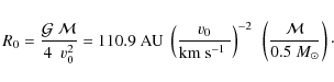
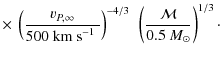
In the solution of V00, the length scale R0 is connected to the mass of the
central object and the velocity normalization via
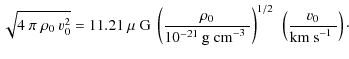
From the velocity and density normalization directly follow the normalizations for the magnetic field and pressure as
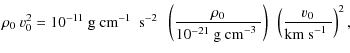
The mass of the central object affects only the length scale. The pressure and temperature of the jet and thus the synthetic emission maps are affected only by the unit density and unit velocity.
As typical jet velocities in YSOs we assumed values of 100, 300, 600 and 1000 km s-1, as typical masses of T Tauri stars 0.2, 0.5 and 0.8 ![]() (Hartigan et al. 1995), and as jet number densities values of 125, 500, 1000 and
(Hartigan et al. 1995), and as jet number densities values of 125, 500, 1000 and
![]() cm-3. We adopt the nomenclature for our runs as e.g.
(
cm-3. We adopt the nomenclature for our runs as e.g.
(
![]() ,
,
![]() ,
M) with
,
M) with
![]() in cm-3,
in cm-3,
![]() in km s-1 and M in
in km s-1 and M in ![]() .
.
In order to find the normalizations listed above, we needed to have typical values of jet density and velocity at a certain position (R, z) for a given mass M, and iteratively solved the Eq. (1). Details of this algorithm and also a graphical picture of this approach are given in Appendix A. The normalizations vary from numerical model to numerical model, therefore we used the corresponding different values for each model.
As another constraint, we require that R0 is small enough that the FWHM of the Gaussian of 15 AU is sampled by a reasonable number of pixels. Because the resolution of our numerical simulations was four pixels per R0, requiring at least two pixels per FWHM requires R0 < 30 AU. This limit highly reduces the number of runs, from 576 to 180. The only valid runs are
- (
 , 600, 0.2), (, 600, 0.5), (, 1000, 0.5),
(, 1000, 0.8) for models ADO, SC1a-b, SC2, SC4;
, 600, 0.2), (, 600, 0.5), (, 1000, 0.5),
(, 1000, 0.8) for models ADO, SC1a-b, SC2, SC4;
- (, 600, 0.2), (,600, 0.5), (, 1000, 0.2),
(, 1000, 0.5), (, 1000, 0.8) for models SC1c-f;
- (,
600, 0.2), (,
1000, 0.2), (,
1000, 0.5),
(,
1000, 0.8) for model SC1g;
- (, 100, 0.2) for model SC3;
- no valid runs for model SC5.
3.2 The artefact of limb-brightening
Table 2: R0 in AU of the different OpenSESAMe runs.
After plotting transverse intensity cuts through the convolved emission maps, it can be seen that the maximum emission does not come from the axis, but from a small shell at a finite radius (Fig. 2, left). This effect of limb-brightening, which has been never observed up to now in real protostellar jets, is a direct consequence of the density and pressure/temperature profiles in the analytical solution and is present in all our models and runs, the untruncated model ADO as well as our truncated models. Details of the physical reasons for this behavior are given in Appendix B.
Because the analytical solution is not well defined close to the axis and we had to interpolate it in our numerical simulations, and because it is likely that a stellar wind resides inside the disk wind (Matsakos et al. 2009), we applied the following corrections before running OpenSESAMe:
- we limited the temperature to 104 K in the whole domain;
- we limited the density around the axis by setting the density inside 1 FWHM to its value at 1 FWHM for each z.
![\begin{figure}
\par\includegraphics[width=7.5cm,clip]{11204f2a.cps}\par\vspace*{2mm}
\includegraphics[width=7.5cm,clip]{11204f2b.cps}
\end{figure}](/articles/aa/full_html/2010/08/aa11204-08/img47.png)
|
Figure 2:
Transverse intensity cuts of the convolved [OI] |
| Open with DEXTER | |
4 Do we have to truncate the disk?
![\begin{figure}
\par\includegraphics[width=14.5cm,clip]{11204f3.eps}
\end{figure}](/articles/aa/full_html/2010/08/aa11204-08/img48.png)
|
Figure 3:
Typical output of OpenSESAMe: cuts of the density and temperature,
the electron and SII and OI ion densities and synthetic emission maps of
the [SII] |
| Open with DEXTER | |
![\begin{figure}
\par\includegraphics[width=14.5cm,clip]{11204f4.eps}
\end{figure}](/articles/aa/full_html/2010/08/aa11204-08/img49.png)
|
Figure 4: Dimensionless jet width derived from synthetic [OI] images as a function of distance from the source in model ADO. |
| Open with DEXTER | |
The extracted jet widths in normalized R0 units are plotted in Fig. 4. In each plot we combine runs with equal velocities and
masses, i.e. only varying the density, which result in identical jet widths as
expected. Because we extracted the jet width from a ratio of intensities
by using the FWHM (we divided the maps by the intensity on the axis and check
where the ratio is 0.5), the factor ![]() cancels out.
cancels out.
Much larger changes are present when we compare runs where ![]() is
identical, but v0 varies (top right and bottom left plot) and when we look
for the influence of the mass (plots in each row). The jet widths derived from
synthetic [OI] are identical to those derived from synthetic [SII] images, thus
we show only results based on [OI] images.
is
identical, but v0 varies (top right and bottom left plot) and when we look
for the influence of the mass (plots in each row). The jet widths derived from
synthetic [OI] are identical to those derived from synthetic [SII] images, thus
we show only results based on [OI] images.
The jet widths in R0 increase with increasing velocity. A higher mass reduces the normalized jet width considerably. In run (500, 600, 0.5), as seen in Fig. 3, the extracted jet width does not follow any directly apparent feature in the emissivity maps nor a specific contour line.
After rescaling the jet widths with the appropriate values of R0, we compared
the modeled and observed jet widths in AU (Fig. 5). The
jet widths are now rescaled with R0, which is proportional to the mass and
anti-proportional to v0 (Eq. (1)). Because
![]() is almost constant in our range of R0,
is almost constant in our range of R0,
![]() and v0 can be interchanged. This behavior of R0 is now
dominant, thus the jet width increases with increasing mass and decreases with
increasing jet velocity, although the second effect seems to be of minor
importance.
and v0 can be interchanged. This behavior of R0 is now
dominant, thus the jet width increases with increasing mass and decreases with
increasing jet velocity, although the second effect seems to be of minor
importance.
![\begin{figure}
\par\includegraphics[width=8cm,clip]{11204f5.eps}
\end{figure}](/articles/aa/full_html/2010/08/aa11204-08/img52.png)
|
Figure 5: Jet widths in AU derived from synthetic [OI] images as a function of distance from the source in model ADO; overlaid are the data points of Fig. 1. |
| Open with DEXTER | |
![\begin{figure}
\par\includegraphics[width=14cm,clip]{11204f6.eps}
\end{figure}](/articles/aa/full_html/2010/08/aa11204-08/img53.png)
|
Figure 6:
Synthetic emission maps of the [OI] |
| Open with DEXTER | |
The untruncated ADO model on average gives too large jet widths compared to the
observations of T Tauri jets. The first five data points within 120 AU from the
jet source in DG Tau can be best approximated with run (500, 600, 0.2),
unfortunately our model does not provide results farther out for such a small
R0. At distances above 200 AU, the run (500, 600, 0.5) gives a jet width in
the observed range but only after the first bump, which is intrinsic for
our analytical model. Hartigan et al. (1995) give a mass of DG Tau of 0.67 ![]() ,
i.e. higher than in both models. Although this difference in mass might not be
meaningful, we conclude that to be able to reproduce all jets in our
sample, we need an additional effect which reduces the derived jet width.
,
i.e. higher than in both models. Although this difference in mass might not be
meaningful, we conclude that to be able to reproduce all jets in our
sample, we need an additional effect which reduces the derived jet width.
![\begin{figure}
\par\includegraphics[width=14.5cm,clip]{11204f7.eps}
\end{figure}](/articles/aa/full_html/2010/08/aa11204-08/img54.png)
|
Figure 7: Jet widths in AU derived from synthetic [OI] images as a function of distance from the source in models ADO and SC1a-g, SC2 and SC4 and for runs (500, 600, 0.2), (500, 600, 0.5), (500, 1000, 0.5), (500, 1000, 0.8); overlaid are the data points of Fig. 1. |
| Open with DEXTER | |
5 Effects of outer truncation
First we investigate the effects of outer truncation. Convolved synthetic maps
for the emission in [OI] ![]() 6300 for some numerical models and run
(500, 1000, 0.5) are given in Fig. 6. Truncation
leads to collimation of the emission region with respect to the model ADO
without any truncation.
6300 for some numerical models and run
(500, 1000, 0.5) are given in Fig. 6. Truncation
leads to collimation of the emission region with respect to the model ADO
without any truncation.
Again we extracted the jet width from emission maps like these. The resulting widths derived from the synthetic [OI] images and scaled to AU are presented in Fig. 7. We found similarities in behavior in the truncated models to the untruncated model ADO. The jet widths show again no dependency on the density, as described for model ADO in the previous section. Surprisingly, in models SC1a-c, SC2 and SC4 the runs (500, 600, 0.2) and (500, 1000, 0.5) and also (500, 1000, 0.8) lead to almost similar physical jet widths. The first two also almost coincide in models SC1d-e. As in model ADO, also in the truncated models the run (500, 600, 0.5) has the smallest jet widths (after the first bump). In principle, we can reproduce even smaller values than the observed ones.
6 Effects of inner truncation
In Paper I we also performed numerical simulations, in which we truncated the
analytical solution in the interior, i.e. at an inner truncation radius. The
physical picture behind this scenario is a stellar magnetosphere truncating the
jet-emitting disk. We showed that inner truncation leads to a decrease of the
jet radius and compression of the material in the inner region.
Unfortunately, only one run met our scaling requirements (Sect. 3.1):
model SC3 and run (![]() ,
100, 0.2). For this model, a convolved synthetic
map for the emission in [OI]
,
100, 0.2). For this model, a convolved synthetic
map for the emission in [OI] ![]() 6300 is given in Fig. 8.
6300 is given in Fig. 8.
After rescaling the derived jet width to AU, we found an almost constant width in the range of the observed values. Note that our model does not provide results farther out than 100 AU due to a small R0.
7 Discussion
We studied the jet widths derived from synthetic emission maps in different forbidden lines as the full-width half-maximum of the emission.
We found that the untruncated model ADO of Vlahakis et al. (2000) cannot account for the small jet widths found in recent optical images taken with HST and AO. The density normalization is not important for the resulting measured jet width as long as we are far from the critical regime.
We investigated different effects for reducing the derived jet width: by imposing an outer radius of the launching region of the underlying accreting disk and thus also of the outflow on the observable structure of the jet and by imposing an inner radius of the underlying accretion disk due to interactions with the stellar magnetosphere.
7.1 Outer truncation
![\begin{figure}
\par\includegraphics[width=5.5cm,clip]{11204f8.cps}
\end{figure}](/articles/aa/full_html/2010/08/aa11204-08/img55.png)
|
Figure 8:
Synthetic emission maps of the [OI] |
| Open with DEXTER | |
![\begin{figure}
\par\includegraphics[width=8cm,clip]{11204f9.eps}
\end{figure}](/articles/aa/full_html/2010/08/aa11204-08/img56.png)
|
Figure 9: Jet widths in AU derived from synthetic [OI] images as a function of distance from the source in model SC3 and for run (500, 100, 0.2); overlaid are the data points of Fig. 1. |
| Open with DEXTER | |
We created synthetic images based on our simulations of truncated disk winds (Stute et al. 2008) as well as new simulations and found that the extracted jet widths in the truncated models decrease for models SC1a-1g, compared to those of the untruncated model ADO, as naively expected.
In the present paradigm, jets are emitted only by the inner part of the disk.
Hence in the other parts the disk can be described by a standard accretion
disk (SAD), in the inner parts by a jet-emitting disk (JED). Anderson et al. (2003)
showed that one can estimate the launching region as
| R0 | = | 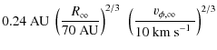
|
|
|
This transition was constrained observationally with measured jet rotation velocities and using the equation above and radii of the order of 0.1-1 AU are used in several theoretical studies as e.g. Combet & Ferreira (2008).
Our results can be used to infer the ``real'' value of the truncation radius
![]() in the observed sample of jets and interpret it as the transition
radius of the JED to the SAD, assuming the specific model of V00 applies.
in the observed sample of jets and interpret it as the transition
radius of the JED to the SAD, assuming the specific model of V00 applies.
At the lower boundary in our simulations, the truncation radii are
given in Table 1. They vary from 5.375 R0 in model SC1a to 0.575 R0 in model SC1g. However, these radii are set at z = 6 R0 (the
lower boundary), not in the equatorial plane. Those can be calculated by
extrapolating the field line, i.e.
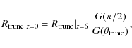
|
(4) |
with
- in models SC1a, SC2-4
 ,
,
- in model SC1b
 ,
,
- in model SC1c
 ,
,
- in model SC1d
 ,
,
- in model SC1e
 ,
,
- in model SC1f
 and
and
- in model SC1g
 .
.
Table 3:
Truncation radius at the equator
![]() in AU of the
different OpenSESAMe runs.
in AU of the
different OpenSESAMe runs.
We found best-fit models for the jets in the observed sample. Note that we always ignored the first bump in the synthetic jet widths and focussed on larger distances from the source:
- the observed mass of DG Tau (diamonds in Fig. 7)
is 0.67
 (Hartigan et al. 1995), therefore we have to focus on the runs
(500, 1000, 0.8), and perhaps also runs (500, 600, 0.5) and (500, 1000, 0.5). The
best-fit model is between ADO and SC1a, thus the truncation radius is larger
than 0.22 AU;
(Hartigan et al. 1995), therefore we have to focus on the runs
(500, 1000, 0.8), and perhaps also runs (500, 600, 0.5) and (500, 1000, 0.5). The
best-fit model is between ADO and SC1a, thus the truncation radius is larger
than 0.22 AU;
- HN Tau (plus signs) has a mass of 0.72
(Hartigan et al. 1995), thus
again the runs (500, 1000, 0.8) are favored. Because we ignored the first bump, we
interpolated the jet shape at larger distances and found a best-fit model
between ADO and SC1a, thus the truncation radius is again larger than 0.34 AU.
However,this result is highly uncertain;
- the mass of CW Tau (squares) is the highest in our sample, 1.03
(Hartigan et al. 1995). Using the runs (500, 1000, 0.8), the best-fit model is SC1b or
SC1c. The truncation radius is thus between 0.25-0.3 AU;
- UZ Tau E (crosses) has the lowest mass in our sample, only 0.18
(Hartigan et al. 1995), we use the runs (500, 600, 0.2). Again we had to interpolate the
jet width from larger distances and choose model SC1a as best-fit model. The
truncation radius is about 0.26 AU;
- the measured mass of RW Aur (circles) is 0.85
(Hartigan et al. 1995),
thus we have to focus on runs (500, 1000, 0.8). We need a very high degree of
truncation as in models SC1e-g, thus a truncation radius of the order of 0.04 AU.
7.2 Inner truncation
Because the jet-emitting accretion disk is thought to be truncated by the
stellar magnetosphere, we also investigated our models in which the analytical
solution is truncated at an inner radius. We found that inner truncation can
also reduce the extracted jet widths. The jet width from our model SC3 and run
(![]() , 100, 0.2) is about 30 AU for the inner 100 AU of the jet. This is well
in the observed range of 15-45 AU. Because we did not vary the inner
truncation radius, we can only claim - based on our results of Paper I - that
the larger the truncation radius, the higher is the compression of the
resulting jet. In our models we chose a radius of 5.375 R0 at z = 6. For
model SC3 and run (
, 100, 0.2) is about 30 AU for the inner 100 AU of the jet. This is well
in the observed range of 15-45 AU. Because we did not vary the inner
truncation radius, we can only claim - based on our results of Paper I - that
the larger the truncation radius, the higher is the compression of the
resulting jet. In our models we chose a radius of 5.375 R0 at z = 6. For
model SC3 and run (![]() , 100, 0.2), this corresponds to an inner truncation
radius of 0.11 AU, which is only slightly higher than the inner hole in T Tauri
disks (0.02-0.07 AU, Najita et al. 2007). A parameter study varying the inner
truncation radius is needed.
, 100, 0.2), this corresponds to an inner truncation
radius of 0.11 AU, which is only slightly higher than the inner hole in T Tauri
disks (0.02-0.07 AU, Najita et al. 2007). A parameter study varying the inner
truncation radius is needed.
8 Conclusions
We showed as a proof of concept that jet widths derived from numerical simulations extending analytical MHD jet formation models can be very helpful for understanding recently observed jet widths from observations with adaptive optics and space telescopes. However, further aspects have to be investigated in more detail.
An intrinsic feature in all our models with outer truncation is the first bump in the extracted jet width, which complicates the comparison of synthetic and observed jet widths. Only for DG Tau and CW Tau, we could unambiguously find models with outer truncation which fitted the observed jet widths at larger distances. For HN Tau and UZ Tau E, we have no observed jet widths at larger distances, only in the region which is contaminated by the bump. RW Aur shows very small observed jet widths at all scales, which cannot be reproduced by any of our models and runs. The derived truncation radii (>0.25 AU) are several times larger than the inner radius of the gaseous disk in T Tauri stars (0.02-0.07 AU, Najita et al. 2007), thus our use of a self-similar disk-wind solution is consistent.
The model with inner truncation gives a synthetic jet width, which is constant
and is within the range of observed widths. Another advantage of this model is
that its flow velocities of the order of 100 km s-1 are closer to
observed values. All models with outer truncation have very high velocities
(>600 km s-1 at our scaling point of
![]() AU and
AU and
![]() AU), several times higher than in that with inner
truncation.
AU), several times higher than in that with inner
truncation.
Because we originally focused only on the effect of outer truncation, we kept the inner truncation radius constant in our models SC3 and SC5. In order to further explore the ability of inner truncation to reproduce the observations, we have to vary the inner truncation radius in a parameter study. Naively, one would expect that the derived jet widths are not decreasing for decreasing truncation radii as for the outer truncation, but are increasing. This, however, has to be tested with new simulations.
In our study, we assumed an inclination of 90![]() of the jet, thus
projection effects may slightly change our results. We will present the results
of such a study in a forthcoming paper.
of the jet, thus
projection effects may slightly change our results. We will present the results
of such a study in a forthcoming paper.
Garcia et al. (2001) showed in their Fig. 1 that the measured jet widths
are mainly characterized by the ejection index ![]() ,
defined by Ferreira (1997).
This is related to the model parameter x of the solution of V00,
,
defined by Ferreira (1997).
This is related to the model parameter x of the solution of V00,
![]() ,
and because in our simulations x = 0.75, we get
,
and because in our simulations x = 0.75, we get
![]() ,
which is intrinsic for a standard disk. In the solution of
Ferreira (1997),
,
which is intrinsic for a standard disk. In the solution of
Ferreira (1997), ![]() also controls the opening of the field lines, because it is
connected to the lever arm
also controls the opening of the field lines, because it is
connected to the lever arm ![]() by
by
![]() .
Garcia et al. (2001) favored cold solutions with values of
.
Garcia et al. (2001) favored cold solutions with values of ![]() between 50-70. If
heating along streamlines is allowed, the relation is broken and also warm
solutions of e.g. Casse & Ferreira (2000b) with smaller
between 50-70. If
heating along streamlines is allowed, the relation is broken and also warm
solutions of e.g. Casse & Ferreira (2000b) with smaller ![]() values of 8 and opening
of streamlines (the ratio of the maximum radius to the initial launch radius)
of about 30 can reproduce the observation. In the solution of V00, we have
values of 8 and opening
of streamlines (the ratio of the maximum radius to the initial launch radius)
of about 30 can reproduce the observation. In the solution of V00, we have
![]() and the maximum opening
and the maximum opening
![]() .
The use of other solutions will
therefore highly influence our results in terms of the outer truncation radius.
.
The use of other solutions will
therefore highly influence our results in terms of the outer truncation radius.
The authors would thank the referee, Sylvie Cabrit, for fruitful discussions, suggestions and comments improving this paper. The present work was supported in part by the European Community's Marie Curie Actions - Human Resource and Mobility within the JETSET (Jet Simulations, Experiments and Theory) network under contract MRTN-CT-2004 005592.
References
- Anderson, J. M., Li, Z.-Y., Krasnopolsky, R., & Blandford, R. D. 2003, ApJ, 590, L107 [NASA ADS] [CrossRef] [Google Scholar]
- Bacciotti, F., & Eislöffel, J. 1999, A&A, 342, 717 [NASA ADS] [Google Scholar]
- Blandford, R. D., & Payne, D. G. 1982, MNRAS, 199, 883 [NASA ADS] [CrossRef] [Google Scholar]
- Cabrit, S., Edwards, S., Strom, S. E., & Strom, K. M. 1990, ApJ, 354, 687 [NASA ADS] [CrossRef] [Google Scholar]
- Cabrit, S., Ferreira, J., & Raga, A. C. 1999, A&A, 343, L61 [Google Scholar]
- Casse, F., & Ferreira, J. 2000a, A&A, 353, 1115 [NASA ADS] [Google Scholar]
- Casse, F., & Ferreira, J. 2000b, A&A, 361, 1178 [NASA ADS] [Google Scholar]
- Combet, C., & Ferreira, J. 2008, A&A, 479, 481 [NASA ADS] [CrossRef] [EDP Sciences] [Google Scholar]
- Dougados, C., Cabrit, S., Lavalley, C., & Menard, F. 2000, A&A, 357, L61 [NASA ADS] [Google Scholar]
- Dougados, C., Cabrit, S., Ferreira, J., et al. 2004, Ap&SS, 293, 45 [NASA ADS] [CrossRef] [Google Scholar]
- Dougados, C. 2008, in Jets from Young Stars II: Clues from High Angular Resolution Observations, ed. F. Bacciotti, E. Whelan, & L. Testi (Berlin Heidelberg: Springer-Verlag), Lecture Notes Phys., 742 [Google Scholar]
- Ferreira, J. 1997, A&A, 319, 340 [NASA ADS] [Google Scholar]
- Ferreira, J. 2007, in Jets from Young Stars: Models and Constraints, ed J. Ferreira, C. Dougados, & E. Whelan (Berlin, Heidelberg: Springer-Verlag), Lecture Notes Phys., 723 [Google Scholar]
- Garcia, P. J. V., Cabrit, S., Ferreira, J., & Binette, L. 2001, A&A, 377, 609 [NASA ADS] [CrossRef] [EDP Sciences] [Google Scholar]
- Gracia, J., Vlahakis, N., & Tsinganos, K. 2006, MNRAS, 367, 201 (GVT06) [NASA ADS] [CrossRef] [Google Scholar]
- Hartigan, P., Edwards, S., & Ghandour, L. 1995, ApJ, 452, 736 [NASA ADS] [CrossRef] [Google Scholar]
- Hartigan, P., Edwards, S., & Pierson, R. 2004, ApJ, 609, 261 [NASA ADS] [CrossRef] [Google Scholar]
- Hartmann, L. 2009, in Protostellar Jets in Context, ed. K. Tsinganos, T. P. Ray, & M. Stute (Berlin, Heidelberg: Springer-Verlag) [Google Scholar]
- Lavalley-Fouquet, C., Cabrit, S., & Dougados, C. 2000, A&A, 356, L41 [NASA ADS] [Google Scholar]
- Livio, M. 2009, in Protostellar Jets in Context, ed. K. Tsinganos, T. P. Ray, & M. Stute (Berlin, Heidelberg: Springer-Verlag) [Google Scholar]
- Matsakos, T., Tsinganos, K., Vlahakis, N., et al. 2008, A&A, 477, 521, M08 [NASA ADS] [CrossRef] [EDP Sciences] [Google Scholar]
- Matsakos, T., Massaglia, S., Trussoni, E., et al. 2009, A&A, 502, 217 [NASA ADS] [CrossRef] [EDP Sciences] [Google Scholar]
- Mignone, A., Bodo, G., Massaglia, S., et al. 2007, ApJS, 170, 228 [Google Scholar]
- Najita, J. R., Carr, J. S., Glassgold, A. E., & Valenti, J. A. 2007, in Protostars and Planets V, ed. B. Reipurth, D. Jewitt, & K. Keil (Tucson: University of Arizona Press), 507 [Google Scholar]
- Ray, T. P., Mundt, R., Dyson, J. E., Falle, S. A. E. G., & Raga, A. C. 1996, ApJ, 468, L103 [NASA ADS] [CrossRef] [Google Scholar]
- Ray, T. P., Dougados, C., Bacciotti, F., et al. 2007, in Protostars and Planets V, ed. B. Reipurth, D. Jewitt, & K. Keil (Tucson: University of Arizona Press), 231 [Google Scholar]
- Stute, M., Tsinganos, K., Vlahakis, N., Matsakos, T., & Gracia, J. 2008, A&A, 491, 339, Paper I [NASA ADS] [CrossRef] [EDP Sciences] [Google Scholar]
- Tzeferacos, P., Ferrari, A., Mignone, A., et al. 2009, MNRAS, 400, 820 [NASA ADS] [CrossRef] [Google Scholar]
- Vlahakis, N., & Tsinganos, K. 1998, MNRAS, 298, 777 [NASA ADS] [CrossRef] [Google Scholar]
- Vlahakis, N., Tsinganos, K., Sauty, C., & Trussoni, E. 2000, MNRAS, 318, 417 [NASA ADS] [CrossRef] [Google Scholar]
- Woitas, J., Ray, T. P., Bacciotti, F., Davis, C. J., & Eislöffel, J. 2002, ApJ, 580, 336 [NASA ADS] [CrossRef] [Google Scholar]
- Zanni, C., Ferrari, A., Rosner, R., Bodo, G., & Massaglia, S. 2007, A&A, 469, 811 [NASA ADS] [CrossRef] [EDP Sciences] [Google Scholar]
Appendix A: Details of the normalization algorithm
![\begin{figure}
\par\includegraphics[width=8cm,clip]{11204fA1.eps}
\end{figure}](/articles/aa/full_html/2010/08/aa11204-08/img78.png)
|
Figure A.1:
Shape of the functions f(i) for all models and of the function
g(i) (thick curve) for
|
| Open with DEXTER | |
In order to find the reference values for the distance R0, pressure p0
and magnetic field B0 listed in Eqs. (1)-(3),
we require some typical values of jet density and velocity at a certain
position - we define the jet as the region at the physical position
![]() AU - and solve iteratively
Eq. (1):
AU - and solve iteratively
Eq. (1):
- 1.
- we start the iteration with the choice R0 = 1 AU, namely in the grid cell (40, 398);
- 2.
- we find v0 by dividing the required jet velocity by the velocity in PLUTO units inside the grid cell;
- 3.
- we calculate R0 with Eq. (1);
- 4.
- we calculate the physical position of the grid cell using this new R0;
- 5.
- if R (z) of the grid cell is larger than 10 AU (100 AU), we move to another grid cell 10% closer to the jet axis (equatorial plane); if R (z) of the grid cell is smaller than 10 AU (100 AU), we move to another grid cell 10% further away;
- 6.
- we stop the iteration when the grid cell does not change anymore between two steps.
|
(A.1) |
Figure A.1 shows f(i) for all models and g(i) for
Reducing the required mass or increasing the required jet velocity shifts
the function g(i) upwards and thus increases i of the intersection point
and decreases R0, until g(i) does not intersect with f(i) anymore
inside the computational domain. For example, we could not find acceptable
sets of normalizations for the runs (![]() ,
1000, 0.2) in models ADO, SC1a-b,
SC2 and SC4; in the models SC1c-g, normalizations were found for all runs.
However, most of these runs were later excluded due to our
requirement of R0 < 30 AU.
,
1000, 0.2) in models ADO, SC1a-b,
SC2 and SC4; in the models SC1c-g, normalizations were found for all runs.
However, most of these runs were later excluded due to our
requirement of R0 < 30 AU.
In the inner truncation models SC3 and SC5, the final value of f(i) is much lower, only about 15, therefore both functions only intersect for small velocities. Again, most of the runs found were later excluded due to our requirement of R0 < 30 AU.
Appendix B: Reasons for the artefact of limb-brightening
If the number density is below the critical density, the emissivity of e.g. the
[SII] ![]() 6731 line can be written as
6731 line can be written as
with
with a powerlaw and an exponential cut-off. One can show that
Thus the main emission comes only from a thin shell of the jet, in which the
temperature is exactly in the range of
![]() K. By changing the
temperature normalization, we can move the emitting shell on the axis, but
the resulting jet widths are of the order of the FWHM of the Gaussian PSF.
Therefore we have to have a constant temperature profile towards the axis.
K. By changing the
temperature normalization, we can move the emitting shell on the axis, but
the resulting jet widths are of the order of the FWHM of the Gaussian PSF.
Therefore we have to have a constant temperature profile towards the axis.
Appendix C: Emission maps of the [OI]  6300 line for all models and runs
Here we present the emission maps of the [OI] ![]() 6300 line for all models
and runs (500,
6300 line for all models
and runs (500, ![]() ,
,
![]() )
for the sake of completeness.
)
for the sake of completeness.
| Figure C.1:
Synthetic emission maps of the [OI] |
|
| Open with DEXTER | |
| Figure C.2:
Synthetic emission maps of the [OI] |
|
| Open with DEXTER | |
| Figure C.3:
Synthetic emission maps of the [OI] |
|
| Open with DEXTER | |
| Figure C.4:
Synthetic emission maps of the [OI] |
|
| Open with DEXTER | |
| Figure C.5:
Synthetic emission maps of the [OI] |
|
| Open with DEXTER | |
| Figure C.6:
Synthetic emission maps of the [OI] |
|
| Open with DEXTER | |
| Figure C.7:
Synthetic emission maps of the [OI] |
|
| Open with DEXTER | |
| Figure C.8:
Synthetic emission maps of the [OI] |
|
| Open with DEXTER | |
| Figure C.9:
Synthetic emission maps of the [OI] |
|
| Open with DEXTER | |
![\begin{figure}
\par\includegraphics[width=4.7cm,clip]{11204fC10.cps}
\vspace*{9mm}
\end{figure}](/articles/aa/full_html/2010/08/aa11204-08/img101.png)
|
Figure C.10:
Synthetic emission maps of the [OI] |
| Open with DEXTER | |
| Figure C.11:
Synthetic emission maps of the [OI] |
|
| Open with DEXTER | |
Footnotes
- ...
code
![[*]](/icons/foot_motif.png)
- http://plutocode.to.astro.it/
- ... parameters
- Strictly speaking this is only true when all lengths are also scaled, but because only the gravity term explicitly depends on the length scale and in our case the gravitational force is small compared to the other forces, this slight inconsistency is unimportant (see Paper I).
- ...
OpenSESAMe
- http://homepages.dias.ie/ /jgracia/OpenSESAMe/
All Tables
Table 1: List of numerical science models.
Table 2: R0 in AU of the different OpenSESAMe runs.
Table 3:
Truncation radius at the equator
![]() in AU of the
different OpenSESAMe runs.
in AU of the
different OpenSESAMe runs.
All Figures
|
|
Figure 1: Variation of jet width ( FWHM) derived from [SII] and [OI] images as a function of distance from the source. Data points are from CFHT/PUEO and HST/STIS observations of DG Tau (diamonds), HN Tau (plus signs), CW Tau (squares), UZ Tau E (crosses), RW Aur (circles), HH 34 (one triangle), HH 30 (black solid line) and HL Tau (red dashed line); data are taken from Ray et al. (2007) and references therein. |
| Open with DEXTER | |
| In the text | |
|
|
Figure 2:
Transverse intensity cuts of the convolved [OI] |
| Open with DEXTER | |
| In the text | |
|
|
Figure 3:
Typical output of OpenSESAMe: cuts of the density and temperature,
the electron and SII and OI ion densities and synthetic emission maps of
the [SII] |
| Open with DEXTER | |
| In the text | |
|
|
Figure 4: Dimensionless jet width derived from synthetic [OI] images as a function of distance from the source in model ADO. |
| Open with DEXTER | |
| In the text | |
|
|
Figure 5: Jet widths in AU derived from synthetic [OI] images as a function of distance from the source in model ADO; overlaid are the data points of Fig. 1. |
| Open with DEXTER | |
| In the text | |
|
|
Figure 6:
Synthetic emission maps of the [OI] |
| Open with DEXTER | |
| In the text | |
|
|
Figure 7: Jet widths in AU derived from synthetic [OI] images as a function of distance from the source in models ADO and SC1a-g, SC2 and SC4 and for runs (500, 600, 0.2), (500, 600, 0.5), (500, 1000, 0.5), (500, 1000, 0.8); overlaid are the data points of Fig. 1. |
| Open with DEXTER | |
| In the text | |
|
|
Figure 8:
Synthetic emission maps of the [OI] |
| Open with DEXTER | |
| In the text | |
|
|
Figure 9: Jet widths in AU derived from synthetic [OI] images as a function of distance from the source in model SC3 and for run (500, 100, 0.2); overlaid are the data points of Fig. 1. |
| Open with DEXTER | |
| In the text | |
|
|
Figure A.1:
Shape of the functions f(i) for all models and of the function
g(i) (thick curve) for
|
| Open with DEXTER | |
| In the text | |
| |
Figure C.1:
Synthetic emission maps of the [OI] |
| Open with DEXTER | |
| In the text | |
| |
Figure C.2:
Synthetic emission maps of the [OI] |
| Open with DEXTER | |
| In the text | |
| |
Figure C.3:
Synthetic emission maps of the [OI] |
| Open with DEXTER | |
| In the text | |
| |
Figure C.4:
Synthetic emission maps of the [OI] |
| Open with DEXTER | |
| In the text | |
| |
Figure C.5:
Synthetic emission maps of the [OI] |
| Open with DEXTER | |
| In the text | |
| |
Figure C.6:
Synthetic emission maps of the [OI] |
| Open with DEXTER | |
| In the text | |
| |
Figure C.7:
Synthetic emission maps of the [OI] |
| Open with DEXTER | |
| In the text | |
| |
Figure C.8:
Synthetic emission maps of the [OI] |
| Open with DEXTER | |
| In the text | |
| |
Figure C.9:
Synthetic emission maps of the [OI] |
| Open with DEXTER | |
| In the text | |
|
|
Figure C.10:
Synthetic emission maps of the [OI] |
| Open with DEXTER | |
| In the text | |
| |
Figure C.11:
Synthetic emission maps of the [OI] |
| Open with DEXTER | |
| In the text | |
Copyright ESO 2010
Current usage metrics show cumulative count of Article Views (full-text article views including HTML views, PDF and ePub downloads, according to the available data) and Abstracts Views on Vision4Press platform.
Data correspond to usage on the plateform after 2015. The current usage metrics is available 48-96 hours after online publication and is updated daily on week days.
Initial download of the metrics may take a while.