| Issue |
A&A
Volume 515, June 2010
|
|
|---|---|---|
| Article Number | A58 | |
| Number of page(s) | 10 | |
| Section | Stellar structure and evolution | |
| DOI | https://doi.org/10.1051/0004-6361/200913855 | |
| Published online | 09 June 2010 | |
Rotation and convective core overshoot in  Ophiuchi
C. C. Lovekin - M.-J. Goupil
LESIA, Observatoire de Paris-Meudon, UMR8109, Meudon, France
Received 11 December 2009 / Accepted 10 March 2010
Abstract
Context. Recent work on several ![]() Cephei stars has succeeded in constraining both their interior rotation
profile and their convective core overshoot. In particular, a recent
study focusing on
Cephei stars has succeeded in constraining both their interior rotation
profile and their convective core overshoot. In particular, a recent
study focusing on ![]() Ophiuchi has shown that a convective core overshoot parameter of
Ophiuchi has shown that a convective core overshoot parameter of
![]() is required to model the observed pulsation frequencies, significantly higher than for other stars of this type.
is required to model the observed pulsation frequencies, significantly higher than for other stars of this type.
Aims. We investigate the effects of rotation and overshoot in early type main sequence pulsators, such as ![]() Cephei stars, and attempt to use the low order pulsation frequencies to
constrain these parameters. This will be applied to a few test models
and the
Cephei stars, and attempt to use the low order pulsation frequencies to
constrain these parameters. This will be applied to a few test models
and the ![]() Cephei star
Cephei star ![]() Ophiuchi.
Ophiuchi.
Methods. We use the 2D stellar evolution code ROTORC and the 2D
linear adiabatic pulsation code NRO to calculate pulsation frequencies
for 9.5 ![]() models evolved to an age of 15.6 Myr. We calculate low order p-modes (
models evolved to an age of 15.6 Myr. We calculate low order p-modes (
![]() )
for models with a range of rotation rates and convective core overshoot
parameters. These low order modes are the same range of modes observed
in
)
for models with a range of rotation rates and convective core overshoot
parameters. These low order modes are the same range of modes observed
in ![]() Ophiuchi.
Ophiuchi.
Results. Using these models, we find that the convective core
overshoot has a larger effect on the pulsation frequencies than the
rotation, except in the most rapidly rotating models considered. When
the differences in radii are accounted for by scaling the frequencies
by
![]() ,
the effects of rotation diminish, but are not entirely accounted for.
Thus, this scaling emphasizes the differences produced by changing the
convective core overshoot. We find that increasing the convective core
overshoot decreases the large separation, while producing a slight
increase in the small separations. We created a model frequency grid
which spanned several rotation rates and convective core overshoot
values. We used this grid to define a modified
,
the effects of rotation diminish, but are not entirely accounted for.
Thus, this scaling emphasizes the differences produced by changing the
convective core overshoot. We find that increasing the convective core
overshoot decreases the large separation, while producing a slight
increase in the small separations. We created a model frequency grid
which spanned several rotation rates and convective core overshoot
values. We used this grid to define a modified ![]() statistic in order to determine the best fitting parameters from a set
of observed frequencies. Using this statistic, we are able to recover
the rotation velocity and convective core overshoot for a few test
models. We have also performed a ``hare and hound'' exercise to see how
well 1D models can recover these parameters. Finally, we discuss the
case of the
statistic in order to determine the best fitting parameters from a set
of observed frequencies. Using this statistic, we are able to recover
the rotation velocity and convective core overshoot for a few test
models. We have also performed a ``hare and hound'' exercise to see how
well 1D models can recover these parameters. Finally, we discuss the
case of the ![]() Cephei star
Cephei star ![]() Oph. Using the observed frequencies and a fixed mass and metallicity,
we find a lower overshoot than previously determined, with
Oph. Using the observed frequencies and a fixed mass and metallicity,
we find a lower overshoot than previously determined, with
![]() .
Our determination of the rotation rate agrees well with both previous work and observations, around 30 km s-1.
.
Our determination of the rotation rate agrees well with both previous work and observations, around 30 km s-1.
Key words: asteroseismology - stars: oscillations - stars: rotation
1 Introduction
Recently, great progress in the asteroseismology of ![]() Cephei stars has been made thanks to extensive observational campaigns,
which have allowed constraints to be placed on the interior properties
of some of these stars. For example, Aerts et al. (2003) and Aerts et al. (2004b)
have compiled and analyzed 21 years of photometry for V836 Cen,
identifying six frequencies and their degree and order. Subsequent
modeling has placed constraints on the mass, age, metallicity,
convective core overshooting (
Cephei stars has been made thanks to extensive observational campaigns,
which have allowed constraints to be placed on the interior properties
of some of these stars. For example, Aerts et al. (2003) and Aerts et al. (2004b)
have compiled and analyzed 21 years of photometry for V836 Cen,
identifying six frequencies and their degree and order. Subsequent
modeling has placed constraints on the mass, age, metallicity,
convective core overshooting (
![]() )
and internal rotation profile for this star (Dupret et al. 2004). They find strong evidence for
)
and internal rotation profile for this star (Dupret et al. 2004). They find strong evidence for
![]() in the absence of rotational mixing. Although the rotation rate for this star is quite slow, around 2 km s-1, the observed frequencies can not be matched with a uniformly rotating model.
in the absence of rotational mixing. Although the rotation rate for this star is quite slow, around 2 km s-1, the observed frequencies can not be matched with a uniformly rotating model.
A second ![]() Cephei star,
Cephei star, ![]() Eridani, has also been studied extensively with both photometric and spectroscopic campaigns (Aerts et al. 2004a; Handler et al. 2004). Nine modes were detected for this star, including the radial mode and two
Eridani, has also been studied extensively with both photometric and spectroscopic campaigns (Aerts et al. 2004a; Handler et al. 2004). Nine modes were detected for this star, including the radial mode and two ![]() triplets (De Ridder et al. 2004). Modeling of
triplets (De Ridder et al. 2004). Modeling of ![]() Eridani has also shown that non-uniformly rotating models are required (Pamyatnykh et al. 2004; Ausseloos et al. 2004).
As for V836 Cen, this star cannot be uniformly rotating to match the
observed frequencies, and some convective core overshooting may be
required. There is also some indication that the interior chemical
composition is not homogeneous, with Fe overabundant in the driving
zone.
Eridani has also shown that non-uniformly rotating models are required (Pamyatnykh et al. 2004; Ausseloos et al. 2004).
As for V836 Cen, this star cannot be uniformly rotating to match the
observed frequencies, and some convective core overshooting may be
required. There is also some indication that the interior chemical
composition is not homogeneous, with Fe overabundant in the driving
zone.
Several other ![]() Cephei stars have also been successfully modeled. Using observations by the MOST satellite, Aerts et al. (2006) were able to place constraints on the physical parameters of
Cephei stars have also been successfully modeled. Using observations by the MOST satellite, Aerts et al. (2006) were able to place constraints on the physical parameters of ![]() Ceti, including constraining the convective core overshoot (
Ceti, including constraining the convective core overshoot (
![]() ). Seismic modeling of
). Seismic modeling of ![]() CMa has constrained the core overshoot to
CMa has constrained the core overshoot to
![]() ,
as well as placing constraints on the mass and age of the star (Mazumdar et al. 2006).
,
as well as placing constraints on the mass and age of the star (Mazumdar et al. 2006).
Most recently, Briquet et al. (2007) have successfully modeled the ![]() Cephei star
Cephei star ![]() Ophiuchi using rigid rotation.
This star has been the subject of both photometric and spectroscopic campaigns (Briquet et al. 2005; Handler et al. 2005), with 7 frequencies identified. These frequencies are thought to be the radial fundamental, one
Ophiuchi using rigid rotation.
This star has been the subject of both photometric and spectroscopic campaigns (Briquet et al. 2005; Handler et al. 2005), with 7 frequencies identified. These frequencies are thought to be the radial fundamental, one ![]() triplet, and three components of an
triplet, and three components of an ![]() quintuplet based on both spectroscopic and photometric mode identification. Recent independent modeling agrees with the
quintuplet based on both spectroscopic and photometric mode identification. Recent independent modeling agrees with the ![]() identifications, although in some cases they assign a different m to the modes (Daszynska-Daszkiewicz & Walczak 2010). Spectroscopic observations were also used to determine the metallicity of
identifications, although in some cases they assign a different m to the modes (Daszynska-Daszkiewicz & Walczak 2010). Spectroscopic observations were also used to determine the metallicity of ![]() Ophiuchi, with a best value of
Z = 0.0114 using the new Asplund mixture (Briquet et al. 2007). Based on these observations, the best fitting model for
Ophiuchi, with a best value of
Z = 0.0114 using the new Asplund mixture (Briquet et al. 2007). Based on these observations, the best fitting model for ![]() Oph has been found to have a mass of about 8.2
Oph has been found to have a mass of about 8.2 ![]() ,
,
![]() ,
,
![]() ,
,
![]() and a rotational velocity of about 30 km s-1 (Briquet et al. 2007).
and a rotational velocity of about 30 km s-1 (Briquet et al. 2007).
The convective core overshoot determined for ![]() Ophiuchi is surprisingly large,
Ophiuchi is surprisingly large,
![]() .
This result is more than double that found for similar
.
This result is more than double that found for similar ![]() Cephei stars, which have
Cephei stars, which have
![]() around 0.1-0.2. It is possible that the unusually high overshoot is a
result of 1D modeling, which does not take into account rotational
effects on the evolution. Although
around 0.1-0.2. It is possible that the unusually high overshoot is a
result of 1D modeling, which does not take into account rotational
effects on the evolution. Although ![]() Oph is relatively slowly rotating for a B star, its rotation velocity,
Oph is relatively slowly rotating for a B star, its rotation velocity,
![]() km s-1, is significantly higher than the stars discussed above, which have rotation velocities around 2 km s-1 (V836 Cen) and 6 km s-1 (
km s-1, is significantly higher than the stars discussed above, which have rotation velocities around 2 km s-1 (V836 Cen) and 6 km s-1 (![]() Eri). Rotation and convective core overshoot may be complimentary
effects, in which case including rotation could reduce the amount of
convective core overshoot required to match the observed frequencies.
The
Eri). Rotation and convective core overshoot may be complimentary
effects, in which case including rotation could reduce the amount of
convective core overshoot required to match the observed frequencies.
The ![]() of
of ![]() Oph is about 30 km s-1and the star is thought to be viewed nearly equator on (Briquet et al. 2005).
Although this is not particularly rapid rotation for a star of this
type, the rotation should produce some effect on the structure and
frequencies. We have chosen to model
Oph is about 30 km s-1and the star is thought to be viewed nearly equator on (Briquet et al. 2005).
Although this is not particularly rapid rotation for a star of this
type, the rotation should produce some effect on the structure and
frequencies. We have chosen to model ![]() Oph using models which are uniformly rotating on the ZAMS. In this
work, we use 2D stellar evolution and linear adiabatic pulsation codes
to determine the effects of rotation and overshoot on pulsation
frequencies. By including a 2D treatment of rotation, we investigate
whether the overshoot of
Oph using models which are uniformly rotating on the ZAMS. In this
work, we use 2D stellar evolution and linear adiabatic pulsation codes
to determine the effects of rotation and overshoot on pulsation
frequencies. By including a 2D treatment of rotation, we investigate
whether the overshoot of ![]() Oph could be reduced while still matching the observed frequencies.
Oph could be reduced while still matching the observed frequencies.
This paper is organized as follows. In Sect. 2, we discuss the stellar evolution and pulsation calculations. In Sect. 3 we recall the effects of convective overshoot on the structure of the star, and in Sect. 4
we discuss the effects of rotation and overshoot on the observed
frequencies in these models. Using the resulting variation we attempt
to determine the rotation rate and overshoot using the observed
frequencies in Sect. 5. As
asteroseismic modeling is more commonly done using 1D models, we
perform a ``hare and hound'' exercise to determine how different the
results from the two methods can be. This exercise is discussed in
Sect. 6. Finally, we constrain the rotation and overshoot of ![]() Oph in Sect. 7. Our results are summarized in Sect. 8.
Oph in Sect. 7. Our results are summarized in Sect. 8.
2 Numerical method
Our stellar models are calculated using the 2D stellar structure code ROTORC (Deupree 1990,1995). This code takes the conservation equations for mass, energy, 3 components of momentum and the composition together with Poisson's equation and solves them implicitly on a two dimensional finite difference grid using the Henyey method (Henyey et al. 1964). We use OPAL opacities (Iglesias & Rogers 1996) and equation of state (Rogers et al. 1996). Unlike standard 1D stellar evolution codes, ROTORC uses the fractional surface equatorial radius and the colatitude as independent variables. The surface equatorial radius is determined by requiring that the integral of the density over the volume of the model equal the total mass. The surface radius in the other angular zones is calculated by assuming the surface is an equipotential. As the models evolve, angular momentum is conserved locally. Although these models are uniformly rotating on the ZAMS, they become slightly differentially rotating as they evolve. This 2D modeling allows us to calculate the structural changes produced by rigid rotation without making assumptions about the shape a priori.
Based on the calculations of Briquet et al. (2007), the mass of ![]() Oph is around 8.5
Oph is around 8.5 ![]() .
We have found that when rotation is taken into account, more massive
models are generally needed to reach a given temperature and
lumniosity. We have calculated models at 8.5, 9 and 9.5
.
We have found that when rotation is taken into account, more massive
models are generally needed to reach a given temperature and
lumniosity. We have calculated models at 8.5, 9 and 9.5 ![]() ,
and have found that the 9.5
,
and have found that the 9.5 ![]() models gave the best match to the observed temperature and luminosity of
models gave the best match to the observed temperature and luminosity of ![]() Oph. We have calculated a small grid of these 9.5
Oph. We have calculated a small grid of these 9.5 ![]() models evolved to an age of 15.6 Myr. For these calculations, we
used 581 radial zones and 10 angular zones. The fractional surface
equatorial radius was taken to be 1, and the ratio between the polar
and equatorial radii decreases as the rotation rate increases. For the
velocities considered here, the rotational effects are not expected to
be too severe (see Lovekin et al. 2009).
These models are uniformly rotating on the ZAMS, with surface
equatorial velocities on the ZAMS of 0, 50, 100, 150 and
200 km s-1, (corresponding to approximately 0, 35, 65, 110 and 150 km s-1 at 15.6 Myr) and overshoot parameters (
models evolved to an age of 15.6 Myr. For these calculations, we
used 581 radial zones and 10 angular zones. The fractional surface
equatorial radius was taken to be 1, and the ratio between the polar
and equatorial radii decreases as the rotation rate increases. For the
velocities considered here, the rotational effects are not expected to
be too severe (see Lovekin et al. 2009).
These models are uniformly rotating on the ZAMS, with surface
equatorial velocities on the ZAMS of 0, 50, 100, 150 and
200 km s-1, (corresponding to approximately 0, 35, 65, 110 and 150 km s-1 at 15.6 Myr) and overshoot parameters (
![]() )
of 0, 0.08, 0.18, 0.28 and 0.38. We used a metallicity slightly higher than that determined by Briquet et al. (2007) for
)
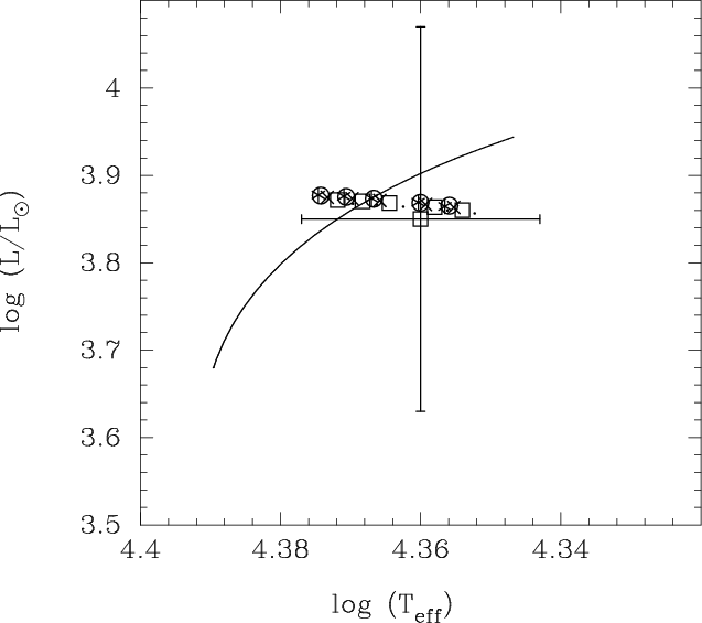
of 0, 0.08, 0.18, 0.28 and 0.38. We used a metallicity slightly higher than that determined by Briquet et al. (2007) for ![]() Oph, with Z = 0.02. The initial hydrogen fraction of these models was 0.7. The properties of these models are summarized in Table 1. The location of these models in the HR diagram is shown in Fig. 1, along with a sample evolution track (v = 0,
Oph, with Z = 0.02. The initial hydrogen fraction of these models was 0.7. The properties of these models are summarized in Table 1. The location of these models in the HR diagram is shown in Fig. 1, along with a sample evolution track (v = 0,
![]() ). The location of
). The location of ![]() Oph with observational error bars from the photometric observations of Handler et al. (2005) is shown for reference.
Oph with observational error bars from the photometric observations of Handler et al. (2005) is shown for reference.
|
Figure 1:
Location in the HR diagram for the 9.5 |
| Open with DEXTER | |
Table 1: Summary of model properties.
To calculate pulsation frequencies, we used a 2D linear adiabatic pulsation code, NRO (Clement 1998). This code solves the linearized pulsation equations on a 2D grid using a finite difference technique. The ROTORC model, which is defined on a spherical polar grid is transformed into a model with the same number of radial zones, but defined on surfaces of constant density. The pulsation equations are rewritten as finite difference expressions and the coefficients are placed in a band diagonal matrix. Each element of this matrix is itself a matrix, containing the coefficients at each zone in the 2D grid. The solution proceeds in two steps, from the centre outwards and from the surface inwards. The solutions are required to match at some intermediate fitting surface. At this point, a discriminant can be evaluated, which will only be satisfied (equal to zero) if an eigenvalue has been located. Frequencies are detected by stepping through frequency space and looking for zero crossings in the value of the discriminant. This method can result in missed frequencies if the frequencies are sufficiently close together, but this can usually be avoided by reducing the frequency step size. For further discussion of the solution mechanism, refer to Lovekin & Deupree (2008); Clement (1998).
In rotating stars, a given mode cannot be described by a single spherical harmonic, but requires a linear combination of
![]() 's.
We can calculate the first few terms in this combination as the
eigenfunctions calculated with NRO are given as a function of r and
's.
We can calculate the first few terms in this combination as the
eigenfunctions calculated with NRO are given as a function of r and ![]() ,
and are defined at several points on the surface. Up to 9 angular zones
can be included in the calculation, with one radial integration
performed for each angle included. The solution is given at N
angles, which can subsequently be decomposed into the contributions of
individual spherical harmonics, effectively calculating the first N
terms in the linear combination. Each radial integration contains
angular derivatives, evaluated using finite differencing, so the
resultant coupling among spherical harmonics arises naturally. In NRO, specifying
,
and are defined at several points on the surface. Up to 9 angular zones
can be included in the calculation, with one radial integration
performed for each angle included. The solution is given at N
angles, which can subsequently be decomposed into the contributions of
individual spherical harmonics, effectively calculating the first N
terms in the linear combination. Each radial integration contains
angular derivatives, evaluated using finite differencing, so the
resultant coupling among spherical harmonics arises naturally. In NRO, specifying ![]() specifies the parity of the mode, and the calculation is performed using the first N even or odd spherical harmonics. In non-axisymmetric modes, the appropriate spherical harmonics are chosen starting with
specifies the parity of the mode, and the calculation is performed using the first N even or odd spherical harmonics. In non-axisymmetric modes, the appropriate spherical harmonics are chosen starting with ![]() = m.
= m.
Since a given mode in a rotating star is described by a linear
combination of spherical harmonics, the mode no longer has a unique ![]() ,
although m does remain unique. Since
,
although m does remain unique. Since ![]() is no longer unique, some new way of identifying modes must be used. We have chosen to identify modes by the parameter
is no longer unique, some new way of identifying modes must be used. We have chosen to identify modes by the parameter ![]() ,
which is the
,
which is the ![]() of the mode in the non-rotating model to which a given mode can be
traced back. This tracing is done for a series of models of gradually
increasing velocity, based on both the shape of the latitudinal
variation at the surface and the frequency. As the velocity gradually
increases, the resulting distortion increases, allowing the modes to be
identified. However, this process becomes more difficult as the
rotation rate increases, and is described in more detail in Lovekin & Deupree (2008). Similar problems have been encountered by for example, Reese et al. (2009).
of the mode in the non-rotating model to which a given mode can be
traced back. This tracing is done for a series of models of gradually
increasing velocity, based on both the shape of the latitudinal
variation at the surface and the frequency. As the velocity gradually
increases, the resulting distortion increases, allowing the modes to be
identified. However, this process becomes more difficult as the
rotation rate increases, and is described in more detail in Lovekin & Deupree (2008). Similar problems have been encountered by for example, Reese et al. (2009).
We have calculated frequencies for
![]() ,
as shown in Fig. 2 for the non-rotating models. We have chosen these low order p-modes for comparison with the modes detected in
,
as shown in Fig. 2 for the non-rotating models. We have chosen these low order p-modes for comparison with the modes detected in ![]() Oph. The frequencies shown in this plot were scaled by a factor of
Oph. The frequencies shown in this plot were scaled by a factor of
![]() to account for differences in the radii of the models. We have chosen the radius at a colatitude of 40
to account for differences in the radii of the models. We have chosen the radius at a colatitude of 40![]() as this radius has been found to be the radius most appropriate for calculating a pulsation constant in similar models (Lovekin & Deupree 2008).
as this radius has been found to be the radius most appropriate for calculating a pulsation constant in similar models (Lovekin & Deupree 2008).
![\begin{figure}
\par\includegraphics[width=8.6cm,clip]{13855f2.ps}
\end{figure}](/articles/aa/full_html/2010/07/aa13855-09/img54.png)
|
Figure 2:
The calculated frequencies for the non-rotating model; * - |
| Open with DEXTER | |
3 Structural effects
In order to better understand the influence of convective core
overshooting, we have considered the effects of rotation and overshoot
on the stellar structure for a collection of models at the same age. As
seen in Fig. 1 and Table 1,
increasing the convective core overshoot increases both the effective
temperature and luminosity slightly. Increased rotation does the
opposite, causing a slight decrease in temperature and luminosity. This
decrease is small except for the most rapidly rotating model considered
here (200 km s-1). These changes in temperature
and luminosity can be related to the change in the radius of the star.
As the rotation rate increases, the equatorial radius increases, while
the polar radius decreases. This effect is well known, and has been
demonstrated by many other authors (see, for example Deupree 2001; Meynet & Maeder 1997; Bodenheimer 1971).
We have also found that for a given rotation rate, increasing the
convective core overshoot decreases the radius by up to 0.8 ![]() for models at the same age and velocity, despite the corresponding increase in both temperature and luminosity (see Table 1).
for models at the same age and velocity, despite the corresponding increase in both temperature and luminosity (see Table 1).
To help us assess the effect of changing core overshoot on the
structure, and hence the frequencies, we have calculated the
Brunt-V"ais"al"a frequency, defined as
![\begin{displaymath}N^2 = g\left[\frac{1}{P\Gamma_1}\frac{\partial P}{\partial r} - \frac{1}{\rho}\frac{\partial \rho}{\partial r}\right]
\end{displaymath}](/articles/aa/full_html/2010/07/aa13855-09/img55.png)
|
(1) |
for each of our models. In Fig. 3, we show N2/g for a non-rotating model and a rapidly rotating model (200 km s-1) with no convective core overshooting. The small wiggles visible, particularly in the outer sections of the star, are purely numerical effects, resulting from the finite difference calculation of the derivative. The main peak at the boundary of the convective core has approximately the same size and shape in both models. Clearly, changing the rotation rate does not produce much change in the shape of the normalized Brunt-V"ais"al"a frequency. Although increased rotation increases the absolute size of the convective core, in terms of fractional radius, this size remains roughly constant. In these models, local conservation of momentum means there is little radial mixing, so the composition gradient does not change significantly with rotation rate. Although there are slight differences throughout the envelope of the star, they are small and unlikely to cause large shifts in the frequencies. On the other hand, the overshoot has a much larger effect on the Brunt-V"ais"al"a frequency. Figure 4 shows the Brunt-V"ais"al"a frequency for two non-rotating models with core overshoot parameters of 0 and 0.38. As expected, the peak at the boundary of the convective core has shifted outwards in radius. This region is really the only significant difference, and the Brunt-V"ais"al"a frequencies are similar throughout the envelopes of the models.
![\begin{figure}
\par\includegraphics[width=8.5cm,clip]{13855f3.ps}
\end{figure}](/articles/aa/full_html/2010/07/aa13855-09/img56.png)
|
Figure 3:
The normalized Brunt-V"ais"al"a frequency for a 9.5 |
| Open with DEXTER | |
![\begin{figure}
\par\includegraphics[width=8.5cm,clip]{13855f4.ps}
\end{figure}](/articles/aa/full_html/2010/07/aa13855-09/img57.png)
|
Figure 4:
The normalized Brunt-V"ais"al"a frequency for 9.5 |
| Open with DEXTER | |
4 Effects on the frequencies and frequency separations
Using the 2D stellar evolution and pulsation calculations described in Sect. 2, we have calculated pulsation frequencies for models with rotational velocities from 0-200 km s-1
and overshoot parameters of 0-0.38. Each model was evolved to an age of
15.6 Myr. As the overshoot and rotation change the evolution
slightly, all of these models have slightly different radii and core
hydrogen fraction (![]() ), as discussed in Sect. 3 (see also Table 1 and Fig. 1). In order to offset the effects of this difference, we have scaled the frequencies by a factor of
), as discussed in Sect. 3 (see also Table 1 and Fig. 1). In order to offset the effects of this difference, we have scaled the frequencies by a factor of
![]() when looking for the effects of rotation and convective core overshoot.
We have chosen the radius at this colatitude as it has been found to
produce the best pulsation constant (Lovekin & Deupree 2008), and hence should be the best choice for scaling the frequencies.
when looking for the effects of rotation and convective core overshoot.
We have chosen the radius at this colatitude as it has been found to
produce the best pulsation constant (Lovekin & Deupree 2008), and hence should be the best choice for scaling the frequencies.
4.1 Frequencies
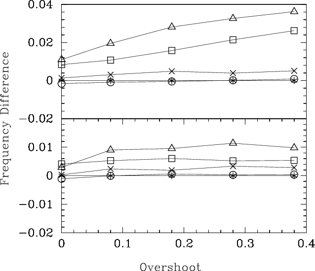
To determine the change in frequency produced by rotation and
overshoot, we have plotted the scaled frequency as a function of
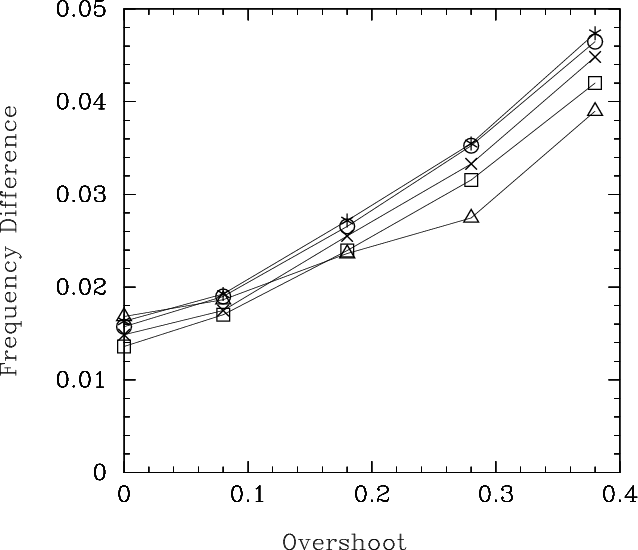
overshoot relative to the non-rotating case (Fig. 5) for the ![]() p1 and p2 modes. The results are similar for the
p1 and p2 modes. The results are similar for the ![]() and 2 modes. In all cases, the differences in scaled frequency produced
by increasing the velocity are small, of order 1-1.5%. This is true
regardless of which radius is used to scale the frequencies. Using the
equatorial radius does not change the results, while when the
frequencies are scaled by the polar radius the magnitude of the
frequency difference is slightly larger. Interestingly, this change in
scaling also changes the sign of the frequency differences. When the
frequencies are scaled by the equatorial radius, the frequencies
increase as the rotation rate increases, while they decrease with
increasing rotation rate when scaled by the polar radius.
and 2 modes. In all cases, the differences in scaled frequency produced
by increasing the velocity are small, of order 1-1.5%. This is true
regardless of which radius is used to scale the frequencies. Using the
equatorial radius does not change the results, while when the
frequencies are scaled by the polar radius the magnitude of the
frequency difference is slightly larger. Interestingly, this change in
scaling also changes the sign of the frequency differences. When the
frequencies are scaled by the equatorial radius, the frequencies
increase as the rotation rate increases, while they decrease with
increasing rotation rate when scaled by the polar radius.
|
Figure 5:
The change in the |
| Open with DEXTER | |
As discussed in Sect. 3,
although the equatorial radius increases as the rotation rate
increases, the polar radius can actually decrease slightly. For
example, while the equatorial radius in the models with no convective
overshoot increases from 6.76 ![]() to 6.85
to 6.85 ![]() as the rotation rate increases from 0 to 200 km s-1, the polar radius actually decreases to 6.68
as the rotation rate increases from 0 to 200 km s-1, the polar radius actually decreases to 6.68
![]() .
This increases the scaling factor as the rotation rate increases, and
so the scaled frequencies actually decrease relative to the
non-rotating case. At a given overshoot, the radius at a colatitude of
40
.
This increases the scaling factor as the rotation rate increases, and
so the scaled frequencies actually decrease relative to the
non-rotating case. At a given overshoot, the radius at a colatitude of
40![]() stays nearly constant, changing by only 0.007
stays nearly constant, changing by only 0.007 ![]() as the velocity increases from 0 to 200 km s-1,
giving us another reason to choose this as the scaling radius. However,
for a given velocity there is no point on the stellar surface at which
the radius stays approximately constant for all overshoots, and scaling
by the radius is not as effective. In this way, our scaling accounts
for the change in radius produced by rotation, but not that produced by
convective core overshooting. As a result, the curves shown in
Fig. 6 are relatively flat as a function of velocity, while the curves shown in Fig. 5
show variation with increasing overshoot. This choice of scaling will
highlight the differences resulting from the overshooting, making them
easier to analyze.
as the velocity increases from 0 to 200 km s-1,
giving us another reason to choose this as the scaling radius. However,
for a given velocity there is no point on the stellar surface at which
the radius stays approximately constant for all overshoots, and scaling
by the radius is not as effective. In this way, our scaling accounts
for the change in radius produced by rotation, but not that produced by
convective core overshooting. As a result, the curves shown in
Fig. 6 are relatively flat as a function of velocity, while the curves shown in Fig. 5
show variation with increasing overshoot. This choice of scaling will
highlight the differences resulting from the overshooting, making them
easier to analyze.
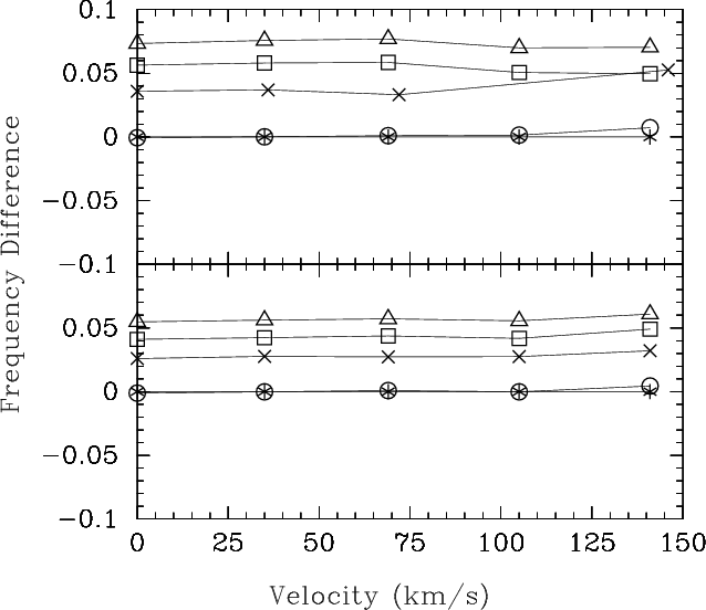
We have also calculated the change in frequency as a function of velocity relative to the case with
![]() ,
shown in Fig. 6, again for the
,
shown in Fig. 6, again for the ![]() p1 and p2
modes. The trends are similar, although larger in magnitude, with the
differences typically of order 10%, as might be expected based on our
choice of scaling. In this case, overshoot appears to affect all
p1 and p2
modes. The trends are similar, although larger in magnitude, with the
differences typically of order 10%, as might be expected based on our
choice of scaling. In this case, overshoot appears to affect all ![]() values equally, as there is little variation with increasing
values equally, as there is little variation with increasing ![]() .
When scaling the frequencies, using the polar radius decreases the
magnitude of the frequency difference slightly, but does not affect the
sign of the frequency difference. Changing the convective core
overshoot does not affect the shape of the star as dramatically as does
rotation, and both the polar and equatorial radii decrease as
.
When scaling the frequencies, using the polar radius decreases the
magnitude of the frequency difference slightly, but does not affect the
sign of the frequency difference. Changing the convective core
overshoot does not affect the shape of the star as dramatically as does
rotation, and both the polar and equatorial radii decrease as
![]() is increased.
is increased.
|
Figure 6:
The change in the |
| Open with DEXTER | |
Both velocity and overshoot can significantly affect the absolute
frequencies, although the effect is almost negligible (less than 1.5%)
with respect to rotation when the frequencies are scaled to account for
differences in radius. The differences shown in Figs. 5 and 6 are scaled using the radius at 40![]() ;
the differences in the unscaled frequencies are about two orders of
magnitude larger. Although the scaled frequencies decrease with
increasing rotation and overshoot, increasing overshoot actually
increases the unscaled frequencies, while increasing velocity causes
the frequencies to decrease. Based on the results here, we find that
the effects of slow to moderate uniform rotation (up to about
200 km s-1)
can be primarily accounted for by the effect on the stellar radius. The
effects of increasing convective core overshoot, on the other hand, are
not so easily accounted for by scaling, and are nearly an order of
magnitude larger than the rotational differences when scaled
frequencies are considered. Although the value of the frequencies
themselves can change significantly, we find that as might be expected,
overshoot produces no effect on the mode splitting.
;
the differences in the unscaled frequencies are about two orders of
magnitude larger. Although the scaled frequencies decrease with
increasing rotation and overshoot, increasing overshoot actually
increases the unscaled frequencies, while increasing velocity causes
the frequencies to decrease. Based on the results here, we find that
the effects of slow to moderate uniform rotation (up to about
200 km s-1)
can be primarily accounted for by the effect on the stellar radius. The
effects of increasing convective core overshoot, on the other hand, are
not so easily accounted for by scaling, and are nearly an order of
magnitude larger than the rotational differences when scaled
frequencies are considered. Although the value of the frequencies
themselves can change significantly, we find that as might be expected,
overshoot produces no effect on the mode splitting.
4.2 Frequency separations
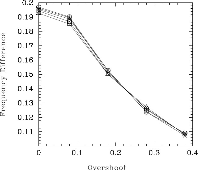
We have also calculated the effect of rotation and overshoot on the
frequency separations. Although the large and small separations are
asymptotic limits, we have applied the definitions to our low order
modes, and continue to refer to these as the large and small
separation. At large radial order, the large separation is defined as
| (2) |
where n is the radial order of the modes. This separation is shown in Fig. 7 for the low order
|
Figure 7:
The large separation for the
|
| Open with DEXTER | |
The small separation is defined as
| (3) |
and shown in Fig. 8 for the even modes. As with the large separation, the small separation decreases slightly as a function of rotation rate up to approximately 200 km s-1. At this velocity, there is a minimum in the small separation, and the small separation increases by approximately 20
|
Figure 8:
The small separations for even (
|
| Open with DEXTER | |
5 Constraining

Once we had established the effects of rotation and overshooting on the
pulsation frequencies and separations, we attempted to determine if
these could be used to constrain a star given a set of observed
frequencies. To do this, we calculated three test models with the same
mass and age as the previous grid of models (see Sect. 2), but with slightly different rotation rates and convective core overshoots: (
![]() ,
,
![]() = (80 km s-1, 0.1), (180 km s-1, 0.1) and (80 km s-1,
0.3). By comparing the differences between the frequencies for these
test models (henceforth the observed frequencies) and the frequencies
in our original grid (model frequencies) we hope to constrain the
rotation and overshoot. Note that throughout this section, we compare
absolute frequencies, not scaled frequencies as in the previous
section.
= (80 km s-1, 0.1), (180 km s-1, 0.1) and (80 km s-1,
0.3). By comparing the differences between the frequencies for these
test models (henceforth the observed frequencies) and the frequencies
in our original grid (model frequencies) we hope to constrain the
rotation and overshoot. Note that throughout this section, we compare
absolute frequencies, not scaled frequencies as in the previous
section.
Initially, we attempted to match individual frequencies. For a given
observed frequency, we calculate the absolute value of the difference
between the observed frequency and each model frequency (
![]() )
and plot this difference versus the observed frequency (
)
and plot this difference versus the observed frequency (
![]() ). All frequencies are normalized by the observed
). All frequencies are normalized by the observed
![]() frequency to offset the effects of varying radius. The results of this calculation are shown in Fig. 9 for the
frequency to offset the effects of varying radius. The results of this calculation are shown in Fig. 9 for the ![]() p1 frequency of the observed
p1 frequency of the observed
![]() km s-1,
km s-1,
![]() case.
The models with the same convective core overshoot parameter cluster in
this diagram, giving no information about the velocity. There is a
clear minimum difference in frequency which falls between
case.
The models with the same convective core overshoot parameter cluster in
this diagram, giving no information about the velocity. There is a
clear minimum difference in frequency which falls between
![]() and 0.18, corresponding to the target overshoot of 0.1.
and 0.18, corresponding to the target overshoot of 0.1.
![\begin{figure}
\par\includegraphics[width=8.5cm,clip]{13855f9.ps}
\end{figure}](/articles/aa/full_html/2010/07/aa13855-09/img70.png)
|
Figure 9:
Determination of overshoot using the |
| Open with DEXTER | |
Using this method, we can of course find a good match for a single
frequency. However, we found that fitting different observed
frequencies from a single observed star can give different results for
the best fitting overshoot. To determine the single best solution for
the rotation and overshoot for each set of observations, we combine the
data for all observed frequencies to determine the best overall fit for
a given model. We do this using a modified ![]() statistic. To calculate this, we compare the observed frequencies to
the calculated frequencies from each model. For a given rotation and
overshoot, we determine the best fitting model frequency for each
observed frequency, where the
statistic. To calculate this, we compare the observed frequencies to
the calculated frequencies from each model. For a given rotation and
overshoot, we determine the best fitting model frequency for each
observed frequency, where the ![]() of the mode is known, but m and n are free parameters. The total
of the mode is known, but m and n are free parameters. The total ![]() for this model is the sum of the differences squared for the
best-fitting matches for the individual frequencies, normalized by the
number of frequencies we fit:
for this model is the sum of the differences squared for the
best-fitting matches for the individual frequencies, normalized by the
number of frequencies we fit:

|
(4) |
where N is the number of frequencies fit for each model. The surface equatorial velocity and core overshoot of the best fit model is given by the lowest overall
This method works best if some additional constraints are applied. Once
a model frequency has been matched to an observed frequency, it is
flagged and considered unavailable for future matches. If more than one
observed frequency is best matched to the same model frequency, we use
a recursive algorithm to determine which arrangement of the frequencies
gives the lowest ![]() .
This also allows us to determine the best fit in cases where we have
more observed frequencies than model frequencies. We also exclude
observed frequencies that are more than 5
.
This also allows us to determine the best fit in cases where we have
more observed frequencies than model frequencies. We also exclude
observed frequencies that are more than 5 ![]() Hz
above (below) the maximum (minimum) value in the model grid. Both of
these constraints remove frequencies from the set of observed
frequencies, and different numbers of frequencies may be removed when
comparing to different models. To account for this, for each overshoot
and velocity, we normalize the
Hz
above (below) the maximum (minimum) value in the model grid. Both of
these constraints remove frequencies from the set of observed
frequencies, and different numbers of frequencies may be removed when
comparing to different models. To account for this, for each overshoot
and velocity, we normalize the ![]() by the number of observed frequencies for which matches were found.
by the number of observed frequencies for which matches were found.
Using this method, we were able to recover the input parameters for our
three ``observed'' models. The observed models have velocities of 80
and 180 km s-1 on the ZAMS, which correspond to 57 or 65 km s-1 (depending on the core overshooting) and 129 km s-1at an age of 15.6 Myr, and overshoot parameters of 0.1 and 0.3 ![]() .
For a model with (v = 129 km s-1,
.
For a model with (v = 129 km s-1,
![]() ), we recovered (110, 0.08), with an uncertainty of
), we recovered (110, 0.08), with an uncertainty of ![]() 50 km s-1 in velocity and
50 km s-1 in velocity and ![]() 0.1
in overshoot due to the coarseness of our model grid. Similarly, for a
model with (57, 0.1) we recovered (65, 0.18) and for a model with (59,
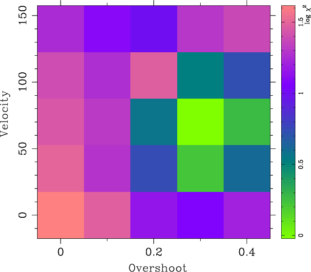
0.3), we recovered (65, 0.28). A sample plot of the
0.1
in overshoot due to the coarseness of our model grid. Similarly, for a
model with (57, 0.1) we recovered (65, 0.18) and for a model with (59,
0.3), we recovered (65, 0.28). A sample plot of the ![]() space is shown in Fig. 10
for a model with parameters (59, 0.3). In general, we find acceptable
solutions over a range of bins, generally straddling the true value. In
the example shown in Fig. 10,
the best solution has a slightly higher velocity and lower overshoot
than the true values, and models with a slightly lower velocity or
higher overshoot are also acceptable solutions.
space is shown in Fig. 10
for a model with parameters (59, 0.3). In general, we find acceptable
solutions over a range of bins, generally straddling the true value. In
the example shown in Fig. 10,
the best solution has a slightly higher velocity and lower overshoot
than the true values, and models with a slightly lower velocity or
higher overshoot are also acceptable solutions.
|
Figure 10:
The log of |
| Open with DEXTER | |
The models shown above were calculated using a full set of calculated
frequencies (about 20 frequencies), including the first two radial
orders for all modes. In more realistic cases, fewer frequencies would
be available, and the m and n
of these modes would be unknown. To examine a more realistic case, we
have created an ``observed'' star with a reduced set of frequencies and
compared them to the full model grid. We have assumed the frequencies
of the ![]() fundamental, a
fundamental, a ![]() triplet and a full
triplet and a full ![]() quintuplet are known (10 frequencies in total). We found that reducing
the number of frequencies in this way did not affect the determination
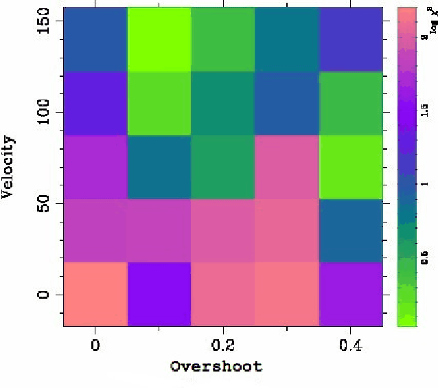
of the best fitting solution. We do find some evidence for a degeneracy
between rotation and overshoot in the most rapidly rotating case, shown
in Fig. 11.
In this case, when only 10 frequencies are included, the best fitting
solution remains in the same area, now at 145 km s-1,
quintuplet are known (10 frequencies in total). We found that reducing
the number of frequencies in this way did not affect the determination
of the best fitting solution. We do find some evidence for a degeneracy
between rotation and overshoot in the most rapidly rotating case, shown
in Fig. 11.
In this case, when only 10 frequencies are included, the best fitting
solution remains in the same area, now at 145 km s-1,
![]() .
A secondary minimum has also appeared, with acceptable solutions having
a core overshoot parameter of 0.38 and a velocity of 65 km s-1.
.
A secondary minimum has also appeared, with acceptable solutions having
a core overshoot parameter of 0.38 and a velocity of 65 km s-1.
|
Figure 11:
The log of |
| Open with DEXTER | |
Clearly, our resolution, particularly in velocity, is very low, and better constraints could be established by using a finer grid. However, even with this coarse resolution, the method successfully returns the correct (albeit uncertain) surface equatorial velocity and core overshoot, at least in cases where the mass and age of the star are known. In general, the mass and age are not known, which will make the fitting process more difficult.
6 Hare and hound exercise
Next, we decided to see how well this determination of rotation and
overshoot could be done using 1D models. This will help quantify the
errors introduced by neglecting rapid rotation in these models. To do
this, low order frequencies were calculated by one of us (CCL) using a
uniformly rotating 2D model as described above. The selected model is
an 8.5 ![]() model, evolved to an age of 20 Myr, with a ZAMS rotation rate of 150 km s-1 (108 km s-1
after 20 Myr). The calculated frequencies and observed position in the
HR diagram were passed on as a set of observational quantities, given
in Table 2. One of us
(MJG) then used these observations to try and determine the convective
core overshoot and rotation rate of the star. The star was assumed to
be a uniformly rotating
model, evolved to an age of 20 Myr, with a ZAMS rotation rate of 150 km s-1 (108 km s-1
after 20 Myr). The calculated frequencies and observed position in the
HR diagram were passed on as a set of observational quantities, given
in Table 2. One of us
(MJG) then used these observations to try and determine the convective
core overshoot and rotation rate of the star. The star was assumed to
be a uniformly rotating ![]() Cephei star oscillating with low order p and g modes with metallicity Z = 0.02. For comparison, we also use the frequencies in Table 2 in a 2D fitting process as described above, assuming the mass and age of the star are known.
Cephei star oscillating with low order p and g modes with metallicity Z = 0.02. For comparison, we also use the frequencies in Table 2 in a 2D fitting process as described above, assuming the mass and age of the star are known.
Table 2: ``Observational'' data used in hare & hound exercise.
In the 1D case, this star was modelled with masses of 8.3 and 8.5 ![]() ,
chosen based on which tracks cross the observed location in the HR
diagram. The calculated evolutionary sequences cross the error box at
an age between 18 and 25 Myr, depending on the amount of
convective core overshoot. Sequences were considered for
,
chosen based on which tracks cross the observed location in the HR
diagram. The calculated evolutionary sequences cross the error box at
an age between 18 and 25 Myr, depending on the amount of
convective core overshoot. Sequences were considered for
![]() ,
0.05, 0.1, 0.2, 0.3 and 0.4. As expected, there is a degeneracy between
mass, age and overshoot in the HR diagram, shown in Fig. 12.
The oscillation code used in this section, WAR(saw)M(eudon), includes
the effects of uniform rotation as a perturbation for axisymmetric
modes as well as frequencies of nonaxisymmetric modes up to third order
in the rotation rate (Daszynska-Daszkiewicz et al. 2002; Soufi et al. 1998; Goupil 2010; Goupil & Talon 2009; Goupil 2009).
Comparison between frequencies obtained with a perturbed approach and a nonperturbative one can be found in Reese et al. (2006); Lignières et al. (2006) for a frequency comparison using the same model, a 2D polytrope, in both approaches, and in Ouazzani et al. (2009) for a comparison using a 1D polytrope in the perturbative approach
and a 2D polytrope involved in the nonperturbative one.
,
0.05, 0.1, 0.2, 0.3 and 0.4. As expected, there is a degeneracy between
mass, age and overshoot in the HR diagram, shown in Fig. 12.
The oscillation code used in this section, WAR(saw)M(eudon), includes
the effects of uniform rotation as a perturbation for axisymmetric
modes as well as frequencies of nonaxisymmetric modes up to third order
in the rotation rate (Daszynska-Daszkiewicz et al. 2002; Soufi et al. 1998; Goupil 2010; Goupil & Talon 2009; Goupil 2009).
Comparison between frequencies obtained with a perturbed approach and a nonperturbative one can be found in Reese et al. (2006); Lignières et al. (2006) for a frequency comparison using the same model, a 2D polytrope, in both approaches, and in Ouazzani et al. (2009) for a comparison using a 1D polytrope in the perturbative approach
and a 2D polytrope involved in the nonperturbative one.
Initially, frequencies were calculated assuming no rotation.
Particularly for the
![]() modes, matching the frequencies was a problem, and for some modes no
solution was found. In this case, the modes identified in Table 2 as p1, p2 and g1 had frequencies corresponding to the p1, g1 and g2 modes in the 1D models. None of the models considered were able to simultaneously fit all of the modes at the same age. A
modes, matching the frequencies was a problem, and for some modes no
solution was found. In this case, the modes identified in Table 2 as p1, p2 and g1 had frequencies corresponding to the p1, g1 and g2 modes in the 1D models. None of the models considered were able to simultaneously fit all of the modes at the same age. A ![]() technique, similar to that described above, was then used to fit all of the modes simultaneously. This
technique, similar to that described above, was then used to fit all of the modes simultaneously. This ![]() fit determined that the 8.3
fit determined that the 8.3 ![]() models gave a better fit to the data, with overshoots of around
models gave a better fit to the data, with overshoots of around
![]() .
The models with the lowest
.
The models with the lowest ![]() have ages between 21-22 Myr, and the temperature and luminosity
are within the observed errors of the target ``star'' (see Fig. 13).
have ages between 21-22 Myr, and the temperature and luminosity
are within the observed errors of the target ``star'' (see Fig. 13).
![\begin{figure}
\par\includegraphics[width=8.5cm,clip]{13855f12.ps}
\end{figure}](/articles/aa/full_html/2010/07/aa13855-09/img80.png)
|
Figure 12:
HR diagram showing the evolutionary tracks (dashed lines) for 8.5 |
| Open with DEXTER | |
![\begin{figure}
\par\includegraphics[width=8.5cm,clip]{13855f13.ps}
\end{figure}](/articles/aa/full_html/2010/07/aa13855-09/img81.png)
|
Figure 13:
The quantity |
| Open with DEXTER | |
The 1D models used in this section are capable of including the effects
of uniform rotation as a perturbation, allowing the mode splitting to
be included. A second ![]() was calculated for the splitting of the models compared to the
``observed'' model. As expected, this splitting was found to be
independent of the overshoot. Good agreement was found for rotation
rates below 125 km s-1, while above this rate the g mode splitting does not agree and
was calculated for the splitting of the models compared to the
``observed'' model. As expected, this splitting was found to be
independent of the overshoot. Good agreement was found for rotation
rates below 125 km s-1, while above this rate the g mode splitting does not agree and ![]() becomes large.
becomes large.
When all effects are included, the 1D modeling finds the best solution to be 8.3 ![]() ,
21 Myr,
,
21 Myr,
![]() and
and
![]() km s-1. In contrast, the 2D modelling described above finds a best fit model with
km s-1. In contrast, the 2D modelling described above finds a best fit model with
![]() and
and
![]() km s-1, given an assumed mass and age of 8.5
km s-1, given an assumed mass and age of 8.5 ![]() and 20 Myr. Solutions at 65 km s-1
are also acceptable, as are core overshoot parameters of 0.18. The
large range in possible velocities found with the 2D models are a
result of the coarseness of the grid, which contains no models with
velocities near 100 km s-1. Although the 1D models
are able to determine the velocity of a target model, the determination
of the overshoot is much less accurate. As discussed in Lignières et al. (2006) and Lovekin & Deupree (2008), for stars rotating more rapidly than about 100 km s-1,
a more accurate treatment of the rotation and pulsation is needed.
These works have shown that a 2D approach tends to produce a larger
effect on the frequencies than 1D perturbative methods. As discussed
above, rotation and overshoot change the unscaled frequencies in
opposite directions. While increasing rotation decreases the
frequencies, increasing core overshoot increases the frequencies.
According to Lovekin & Deupree (2008); Lignières et al. (2006),
1D calculations will not find as large a shift from rotation as 2D
models, and hence will need a smaller overshoot to match the observed
frequency in rapidly rotating stars.
and 20 Myr. Solutions at 65 km s-1
are also acceptable, as are core overshoot parameters of 0.18. The
large range in possible velocities found with the 2D models are a
result of the coarseness of the grid, which contains no models with
velocities near 100 km s-1. Although the 1D models
are able to determine the velocity of a target model, the determination
of the overshoot is much less accurate. As discussed in Lignières et al. (2006) and Lovekin & Deupree (2008), for stars rotating more rapidly than about 100 km s-1,
a more accurate treatment of the rotation and pulsation is needed.
These works have shown that a 2D approach tends to produce a larger
effect on the frequencies than 1D perturbative methods. As discussed
above, rotation and overshoot change the unscaled frequencies in
opposite directions. While increasing rotation decreases the
frequencies, increasing core overshoot increases the frequencies.
According to Lovekin & Deupree (2008); Lignières et al. (2006),
1D calculations will not find as large a shift from rotation as 2D
models, and hence will need a smaller overshoot to match the observed
frequency in rapidly rotating stars.
7 Application to
Oph
Finally, we decided to test the technique discussed in Sect. 5 on ![]() Oph. As discussed in Sect. 5, our resolution in both velocity and overshoot is quite coarse, so we do not expect to place tight constraints on
Oph. As discussed in Sect. 5, our resolution in both velocity and overshoot is quite coarse, so we do not expect to place tight constraints on ![]() Oph in this exploratory calculation. We fixed the metallicity of our models at Z = 0.02, using the Grevesse & Sauval (1998) abundances. For our asteroseismic comparison, we fixed the mass at 9.5
Oph in this exploratory calculation. We fixed the metallicity of our models at Z = 0.02, using the Grevesse & Sauval (1998) abundances. For our asteroseismic comparison, we fixed the mass at 9.5 ![]() ,
after calculating the evolutionary tracks of 8.5, 9 and 9.5
,
after calculating the evolutionary tracks of 8.5, 9 and 9.5 ![]() models and determining which models gave the best match to the observed location of
models and determining which models gave the best match to the observed location of ![]() Oph.
Oph.
The seven observed frequencies of ![]() Oph were compared against the 9.5
Oph were compared against the 9.5 ![]() models shown in Fig. 1, evolved to an age of 15.6 Myr. We used the spectroscopic mode identifications given by Briquet et al. (2005), but used only the given
models shown in Fig. 1, evolved to an age of 15.6 Myr. We used the spectroscopic mode identifications given by Briquet et al. (2005), but used only the given ![]() values as constraints. As for the calculations performed in Sect. 5, we found that the best results were obtained when each frequency is compared only to model frequencies of the same
values as constraints. As for the calculations performed in Sect. 5, we found that the best results were obtained when each frequency is compared only to model frequencies of the same ![]() .
When we do this comparison for
.
When we do this comparison for ![]() Oph, we find the best fit model has a rotation and overshoot of (
Oph, we find the best fit model has a rotation and overshoot of (![]() km s-1,
km s-1,
![]() ). This model is located within the observed photometric errors for
). This model is located within the observed photometric errors for ![]() Oph, with a luminosity of
Oph, with a luminosity of
![]() and an effective temperature
and an effective temperature
![]() K.
The rotation velocity found in our best solution is in good agreement
with the rotation velocity as determined from both the
K.
The rotation velocity found in our best solution is in good agreement
with the rotation velocity as determined from both the ![]() and the observed mode splitting,
and the observed mode splitting, ![]() km s-1 (Briquet et al. 2005,2007). The convective core overshoot determined here is slightly lower than that determined by Briquet et al. (2007),
although the two results do agree within the errors. It seems that when
a more accurate treatment of rotation is taken into account, at least
for slowly rotating stars, this does indeed reduce the need for
convective core overshooting. Our new estimate is still higher than the
results determined for other
km s-1 (Briquet et al. 2005,2007). The convective core overshoot determined here is slightly lower than that determined by Briquet et al. (2007),
although the two results do agree within the errors. It seems that when
a more accurate treatment of rotation is taken into account, at least
for slowly rotating stars, this does indeed reduce the need for
convective core overshooting. Our new estimate is still higher than the
results determined for other ![]() Cephei stars (typically 0.1-0.2), although again, the results agree to within our uncertainties.
Cephei stars (typically 0.1-0.2), although again, the results agree to within our uncertainties.
![\begin{figure}
\par\includegraphics[width=8.5cm,clip]{13855f14.ps}
\end{figure}](/articles/aa/full_html/2010/07/aa13855-09/img89.png)
|
Figure 14:
Log |
| Open with DEXTER | |
Our models for ![]() Oph have been calculated using a metallicity of Z = 0.02 at the composition of Grevesse & Sauval (1998), considerably higher than that determined by Briquet et al. (2007).
As discussed in their work, higher metallicity is correlated to lower
convective core overshoot, so one would expect our models to have a
lower overshoot. In fact, based on the results given in their Table 4,
we would expect a 1D model with our metallicity to have an overshoot of
Oph have been calculated using a metallicity of Z = 0.02 at the composition of Grevesse & Sauval (1998), considerably higher than that determined by Briquet et al. (2007).
As discussed in their work, higher metallicity is correlated to lower
convective core overshoot, so one would expect our models to have a
lower overshoot. In fact, based on the results given in their Table 4,
we would expect a 1D model with our metallicity to have an overshoot of
![]() .
As is expected, this is lower than the overshoot calculated by Briquet et al. (2007),
and is much closer to the value obtained with our 2D models.
Nevertheless, our models also show the need for an unusually high
convective core overshoot in this star. Although our models have shown
some indications that rotation and overshoot can be complimentary
effects, it appears that more rapid rotation is required in order to
influence the frequencies.
.
As is expected, this is lower than the overshoot calculated by Briquet et al. (2007),
and is much closer to the value obtained with our 2D models.
Nevertheless, our models also show the need for an unusually high
convective core overshoot in this star. Although our models have shown
some indications that rotation and overshoot can be complimentary
effects, it appears that more rapid rotation is required in order to
influence the frequencies.
Another limitation of our models is the restriction to fixed mass and
age. This is of course not realistic, and has been introduced to limit
the computations required. As mentioned in Sect. 2, we initially calculated models at three different masses, 8.5, 9 and 9.5 ![]() .
All of these models were close to the observed error box of
.
All of these models were close to the observed error box of ![]() Oph, although the lower mass models needed to be evolved to a higher
age. Although detailed frequency calculations were not performed for
these models, it seems likely that matching models could be found.
Including mass and age as free parameters is currently under
investigation and will be included in future work.
Oph, although the lower mass models needed to be evolved to a higher
age. Although detailed frequency calculations were not performed for
these models, it seems likely that matching models could be found.
Including mass and age as free parameters is currently under
investigation and will be included in future work.
8 Conclusions
We have found that both rotation and overshoot do have an effect on stellar frequencies, although this is predominately through the effects of changing stellar radius. Increasing convective core overshoot increases the unscaled frequencies, while rotation causes the unscaled frequencies to decrease, although certain choices of scaling can minimize this effect for rotation. Although the frequencies themselves may change, as expected we find that the overshoot has no effect on the mode splitting.
We also investigated the effect of overshooting on the large and small separations. We find that increasing convective core overshoot decreases the large separations, but increases the small separation. Unfortunately, both of these effects are similar to the effects of rotation noted by Lovekin et al. (2009), and may not be useful for disentangling the effects of rotation and overshoot.
We have attempted to use the changes in frequency to constrain the best
fitting convective core overshoot. Using individual modes, we were able
to easily constrain the convective core overshoot, although not the
rotation. As should be expected, different modes gave different
results, so we developed a modified ![]() statistic, simultaneously fitting all known frequencies for models of known mass and age (9.5
statistic, simultaneously fitting all known frequencies for models of known mass and age (9.5 ![]() ,
15.6 Myr). We found this was most effective if the
,
15.6 Myr). We found this was most effective if the ![]() s of all frequencies were known. When the
s of all frequencies were known. When the ![]() s
are included, we are able to correctly determine both rotation and
overshoot for models in our grid as well as for three test models with
slightly different
s
are included, we are able to correctly determine both rotation and
overshoot for models in our grid as well as for three test models with
slightly different
![]() and
and
![]() .
Although the uncertainties on our results are large as a result of the
coarse grid spacing used, in all cases the best solutions surrounded
the true parameters of the test models.
.
Although the uncertainties on our results are large as a result of the
coarse grid spacing used, in all cases the best solutions surrounded
the true parameters of the test models.
We also conducted a hare and hound exercise using frequencies calculated using 2D stellar models and pulsation calculations. We found that using 1D stellar models, we were able to find a model that reproduced the frequencies for reasonably close values of age, mass, rotation and convective core overshoot. The 1D models were able to find a velocity quite close to the true rotation rate, although the determination of core overshoot was not as accurate. For a model with true parameters (108, 0.25), the 1D models returned a best fit of (125, 0.1), while the 2D models found a best fit of (145, 0.28). The mass and age returned by the 1D models were also quite close to the true values.
Finally, we applied these methods to ![]() Oph, a rotating
Oph, a rotating ![]() Cephei star with seven observed frequencies. Using models at a fixed
mass and metallicity, we find an overshoot slightlylower than that
determined by Briquet et al. (2007), with
Cephei star with seven observed frequencies. Using models at a fixed
mass and metallicity, we find an overshoot slightlylower than that
determined by Briquet et al. (2007), with
![]() ,
as expected for our higher metallicity models. The rotation velocity
for this model agrees well with the observed value, around
30 km s-1. We also find that a good match to
,
as expected for our higher metallicity models. The rotation velocity
for this model agrees well with the observed value, around
30 km s-1. We also find that a good match to ![]() Oph requires a more massive star than determined by Briquet et al. (2007), around 9.5
Oph requires a more massive star than determined by Briquet et al. (2007), around 9.5 ![]() vs. 8.2
vs. 8.2 ![]() in their models. This difference in mass could be a a consequence of
including rotation in our models, which tends to make models appear
less massive, but may also be a result of the higher metallicity used
in our models. Decreasing the convective core overshoot from 0.44 to
0.28
in their models. This difference in mass could be a a consequence of
including rotation in our models, which tends to make models appear
less massive, but may also be a result of the higher metallicity used
in our models. Decreasing the convective core overshoot from 0.44 to
0.28 ![]() brings
brings ![]() Oph closer to the range of overshoots found in other
Oph closer to the range of overshoots found in other ![]() Cephei stars, around 0.1-0.2
Cephei stars, around 0.1-0.2 ![]() ,
but is still high.
,
but is still high.
As discussed above, (Sect. 6),
the fact that the 1D calculation returns a lower overshoot than the 2D
models while the 1D calculations find a higher overshoot for ![]() Oph is probably a result of the 1D treatment of rotation. At slow rotation velocities (<100 km s-1), like
Oph is probably a result of the 1D treatment of rotation. At slow rotation velocities (<100 km s-1), like ![]() Oph, the 1D method works well, while for more rapidly rotating models,
as in the hare and hound exercise performed here, the 1D treatment of
rotation results in an underestimate of the convective core overshoot.
Oph, the 1D method works well, while for more rapidly rotating models,
as in the hare and hound exercise performed here, the 1D treatment of
rotation results in an underestimate of the convective core overshoot.
The authors acknowledge financial support from the French National Research Agency (ANR) for the SIROCO (SeIsmology, ROtation and COnvection with the COROT satellite ) project.
References
- Aerts, C., Thoul, A., Scuflaire, R., et al. 2003, Science, 300, 1926 [NASA ADS] [CrossRef] [PubMed] [Google Scholar]
- Aerts, C., De Cat, P., Handler, G., et al. 2004a, MNRAS, 347, 463 [NASA ADS] [CrossRef] [Google Scholar]
- Aerts, C., Waelkens, C., Daszynska-Daszkiewicz, J., et al. 2004b, A&A, 415, 241 [NASA ADS] [CrossRef] [EDP Sciences] [Google Scholar]
- Aerts, C., Marchenko, S. V., Matthews, J. M., et al. 2006, ApJ, 642, 470 [NASA ADS] [CrossRef] [Google Scholar]
- Ausseloos, M., Scuflaire, R., Thoul, A., & Aerts, C. 2004, MNRAS, 355, 352 [NASA ADS] [CrossRef] [Google Scholar]
- Bodenheimer, P. 1971, ApJ, 167, 153 [NASA ADS] [CrossRef] [Google Scholar]
- Briquet, M., Lefever, K., Uytterhoeven, K., & Aerts, C. 2005, MNRAS, 362, 619 [NASA ADS] [CrossRef] [Google Scholar]
- Briquet, M., Morel, T., Thoul, A., et al. 2007, MNRAS, 381, 1482 [NASA ADS] [CrossRef] [Google Scholar]
- Clement, M. J. 1998, ApJS, 116, 57 [NASA ADS] [CrossRef] [Google Scholar]
- Daszynska-Daszkiewicz, J., Dziembowski, W. A., Pamyatnykh, A. A., & Goupil, M. 2002, A&A, 392, 151 [NASA ADS] [CrossRef] [EDP Sciences] [Google Scholar]
- Daszynska-Daszkiewicz, J., & Walczak, P. 2010, MNRAS, 98 [Google Scholar]
- De Ridder, J., Telting, J. H., Balona, L. A., et al. 2004, MNRAS, 351, 324 [NASA ADS] [CrossRef] [Google Scholar]
- Deupree, R. G. 1990, ApJ, 357, 175 [NASA ADS] [CrossRef] [Google Scholar]
- Deupree, R. G. 1995, ApJ, 439, 357 [NASA ADS] [CrossRef] [Google Scholar]
- Deupree, R. G. 2001, ApJ, 552, 268 [NASA ADS] [CrossRef] [Google Scholar]
- Dupret, M.-A., Thoul, A., Scuflaire, R., et al. 2004, A&A, 415, 251 [NASA ADS] [CrossRef] [EDP Sciences] [Google Scholar]
- Goupil, M. J. 2009, Lect. Notes Phys., 765, 45 [NASA ADS] [CrossRef] [Google Scholar]
- Goupil, M. J. 2010, Lect. Notes Phys., in press [Google Scholar]
- Goupil, M. J., & Talon, S. 2009, Commun. Asteroseismol., 158, 220 [NASA ADS] [Google Scholar]
- Grevesse, N., & Sauval, A. J. 1998, Space Sci. Rev., 85, 161 [NASA ADS] [CrossRef] [Google Scholar]
- Handler, G., Shobbrook, R. R., Jerzykiewicz, M., et al. 2004, MNRAS, 347, 454 [NASA ADS] [CrossRef] [Google Scholar]
- Handler, G., Shobbrook, R. R., & Mokgwetsi, T. 2005, MNRAS, 362, 612 [NASA ADS] [CrossRef] [Google Scholar]
- Henyey, L., Forbes, J., & Gould, N. 1964, ApJ, 139, 306 [NASA ADS] [CrossRef] [Google Scholar]
- Iglesias, C. A., & Rogers, F. J. 1996, ApJ, 464, 943 [NASA ADS] [CrossRef] [Google Scholar]
- Lignières, F., Rieutord, M., & Reese, D. 2006, A&A, 455, 607 [NASA ADS] [CrossRef] [EDP Sciences] [Google Scholar]
- Lovekin, C. C., & Deupree, R. G. 2008, ApJ, 679, 1499 [NASA ADS] [CrossRef] [Google Scholar]
- Lovekin, C. C., Deupree, R. G., & Clement, M. J. 2009, ApJ, 693, 677 [NASA ADS] [CrossRef] [Google Scholar]
- Mazumdar, A., Briquet, M., Desmet, M., & Aerts, C. 2006, A&A, 459, 589 [NASA ADS] [CrossRef] [EDP Sciences] [Google Scholar]
- Meynet, G., & Maeder, A. 1997, A&A, 321, 465 [NASA ADS] [Google Scholar]
- Ouazzani, R., Goupil, M., Dupret, M., & Reese, D. 2009, Commun. Asteroseismol., 158, 283 [NASA ADS] [Google Scholar]
- Pamyatnykh, A. A., Handler, G., & Dziembowski, W. A. 2004, MNRAS, 350, 1022 [NASA ADS] [CrossRef] [Google Scholar]
- Reese, D., Lignières, F., & Rieutord, M. 2006, A&A, 455, 621 [NASA ADS] [CrossRef] [EDP Sciences] [Google Scholar]
- Reese, D. R., Thompson, M. J., MacGregor, K. B., et al. 2009, A&A, 506, 183 [NASA ADS] [CrossRef] [EDP Sciences] [Google Scholar]
- Rogers, F. J., Swenson, F. J., & Iglesias, C. A. 1996, ApJ, 456, 902 [NASA ADS] [CrossRef] [Google Scholar]
- Soufi, F., Goupil, M. J., & Dziembowski, W. A. 1998, A&A, 334, 911 [NASA ADS] [Google Scholar]
All Tables
Table 1: Summary of model properties.
Table 2: ``Observational'' data used in hare & hound exercise.
All Figures
|
|
Figure 1:
Location in the HR diagram for the 9.5 |
| Open with DEXTER | |
| In the text | |
|
|
Figure 2:
The calculated frequencies for the non-rotating model; * - |
| Open with DEXTER | |
| In the text | |
|
|
Figure 3:
The normalized Brunt-V"ais"al"a frequency for a 9.5 |
| Open with DEXTER | |
| In the text | |
|
|
Figure 4:
The normalized Brunt-V"ais"al"a frequency for 9.5 |
| Open with DEXTER | |
| In the text | |
|
|
Figure 5:
The change in the |
| Open with DEXTER | |
| In the text | |
|
|
Figure 6:
The change in the |
| Open with DEXTER | |
| In the text | |
|
|
Figure 7:
The large separation for the
|
| Open with DEXTER | |
| In the text | |
|
|
Figure 8:
The small separations for even (
|
| Open with DEXTER | |
| In the text | |
|
|
Figure 9:
Determination of overshoot using the |
| Open with DEXTER | |
| In the text | |
|
|
Figure 10:
The log of |
| Open with DEXTER | |
| In the text | |
|
|
Figure 11:
The log of |
| Open with DEXTER | |
| In the text | |
|
|
Figure 12:
HR diagram showing the evolutionary tracks (dashed lines) for 8.5 |
| Open with DEXTER | |
| In the text | |
|
|
Figure 13:
The quantity |
| Open with DEXTER | |
| In the text | |
|
|
Figure 14:
Log |
| Open with DEXTER | |
| In the text | |
Copyright ESO 2010
Current usage metrics show cumulative count of Article Views (full-text article views including HTML views, PDF and ePub downloads, according to the available data) and Abstracts Views on Vision4Press platform.
Data correspond to usage on the plateform after 2015. The current usage metrics is available 48-96 hours after online publication and is updated daily on week days.
Initial download of the metrics may take a while.