| Issue |
A&A
Volume 515, June 2010
|
|
|---|---|---|
| Article Number | A36 | |
| Number of page(s) | 11 | |
| Section | Stellar structure and evolution | |
| DOI | https://doi.org/10.1051/0004-6361/200913729 | |
| Published online | 04 June 2010 | |
Giant pulses from the Crab pulsar
A wide-band study
R. Karuppusamy1,3 - B. W. Stappers2,3 - W. van Straten4
1 - Sterrenkunde Instituut Anton Pannenkoek, University of Amsterdam,
Kruislaan 403, Amsterdam, The Netherlands
2 - Jodrell Bank Centre for Astrophysics, School of Physics and
Astronomy, The University of Manchester, Manchester M13 9PL, UK
3 - Stichting ASTRON, Postbus 2, 7990 AA, Dwingeloo, The Netherlands
4 - Centre for Astrophysics and Supercomputing, Swinburne University of
Technology, Hawthorn, VIC 3122, Australia
Received 24 November 2009 / Accepted 7 February 2010
Abstract
The Crab pulsar is well-known for its anomalous giant radio pulse
emission. Past studies have concentrated only on the very bright pulses
or were insensitive to the faint end of the giant pulse luminosity
distribution. With our new instrumentation offering a large bandwidth
and high time resolution combined with the narrow radio beam of the
Westerbork Synthesis Radio Telescope (WSRT), we seek to probe the weak
giant pulse emission regime. The WSRT was used in a phased array mode,
resolving a large fraction of the Crab nebula. The resulting pulsar
signal was recorded using the PuMa II pulsar backend and then
coherently dedispersed and searched for giant pulse emission. After
careful flux calibration, the data were analysed to study the giant
pulse properties. The analysis includes the distributions of the
measured pulse widths, intensities, energies, and scattering times. The
weak giant pulses are shown to form a separate part of the intensity
distribution. The large number of giant pulses detected were used to
analyse scattering and scintillation in giant pulses. We report for the
first time the detection of giant pulse emission at both the main- and
interpulse phases within a single rotation period. The rate of
detection is consistent with the appearance of pulses at either pulse
phase as being independent. These pulse pairs were used to examine the
scintillation timescales within a single pulse period.
Key words: pulsars: individual: Crab pulsar
1 Introduction
Identified as the supernova remnant that resulted from SN 1054, the Crab nebula is one of the strongest radio sources in the sky, and it harbours the young neutron star PSR B0531+21. The pulsar is visible across the entire observable electromagnetic spectrum, and at radio wavelengths it is the second brightest pulsar in the northern sky. PSR B0531+21 was discovered by Staelin & Reifenstein (1968), soon after the discovery of pulsars. This pulsar is noted for several features including the near orthogonal alignment of the magnetic and rotational axis that gives rise to the observed interpulse emission. The average emission profile of the pulsar, obtained by averaging the radio emission from many rotations of the star, exhibits a number of features that change quite remarkably with radio frequency (Moffett & Hankins 1994). The single pulses show a large variation in amplitude and duration as a function of time. The most enigmatic of these are its occassional intense bursts known as giant pulses (Staelin & Sutton 1970; Heiles et al. 1970). The giant pulses can be extremely narrow, of the order of 0.4 ns (Hankins & Eilek 2007) and the pulse flux can be several 1000 times the average pulse flux. The ultrashort durations of the giant pulses imply very high equivalent brightness temperatures (Hankins et al. 2003) indicating that they originate from nonthermal, coherent emission processes. In this work, we define giant pulses as the pulses with a significantly narrower width than the average emission and contain a flux of at least 10 times the mean flux density of the pulsar.
The Crab pulsar is one of just a handful of pulsars that have been shown to have giant pulse emission. Some other pulsars, like the young Vela pulsar, also show narrow, bursty emission called giant micropulses (Johnston et al. 2001). The fluxes of these micropulses are within a factor of 3 times the average pulse flux. In the pulsars that show giant pulse emission, the pulse intensity and energy distributions exhibit power-law statistics (Argyle & Gower 1972), while the giant micropulses give rise to log-normal distributions (Cairns et al. 2001). In contrast, the bulk of the pulsar population have pulse intensities and energies that follow either a normal or an exponential distribution (Ritchings 1976; Hesse & Wielebinski 1974). This indicates that the giant pulses and micropulses may form a different emission population.
The Crab giant pulses have been studied by different groups, yet the nature of the emission process remains elusive. In the very early studies at low sky frequencies, the data were afflicted by dispersion smearing and scattering (Heiles et al. 1970; Gower & Argyle 1972), but the power-law nature of the intensity distribution of giant pulses was identified. In the next major study, Lundgren et al. (1995) discuss a multi-wavelength observation of giant pulse emission, and note the possibility of a weak giant pulse emission population at radio wavelengths, which they are unable to resolve owing to insufficient sensitivity. Sallmen et al. (1999) found that the Crab giant pulses are broad band at radio wavelengths. They also determine giant pulse spectral indices in the range of -2.2 to -4.9 using their widely spaced observation bands and 29 simultaneously detected giant pulses. Observations by Hankins et al. (2003) revealed that giant pulses at 5.5 GHz contain nanosecond wide subpulses and the presence of such narrow features has been predicted in numerical modelling by Weatherall (1998). At these frequencies the radio emission character of the Crab pulsar changes, with the interpulse emission becoming dominant. A multi-wavelength radio observation of Crab giant pulses with widely spaced frequency bands (0.43 GHz and 8.8 GHz) is presented by Cordes et al. (2004), who discuss the effects of scintillation over a wide range of frequencies. Popov & Stappers (2007) and Eilek et al. (2002) investigated pulse width distributions and find that narrow pulses tend to be brighter. Bhat et al. (2008) carried out a similar analysis in addition to scattering and dispersion variations in the nebula. All of these studies point to the peculiarity of the Crab pulsar and its puzzling emission process, and motivates further study in finer detail using a large number of pulses. For the work discussed in this paper, we utilised the wide band capabilities of the new pulsar machine, PuMa-II (Karuppusamy et al. 2008) and the Westerbork Synthesis Radio Telescope (WSRT) in the coherent tied-array mode. At small hour angles, the synthesised beam of the WSRT effectively resolves out the Crab nebula, reducing the nebular contribution to the system temperature. Thus the WSRT and PuMa-II combination makes this study much more sensitive in terms of signal-to-noise ratio achieved, and in number of pulses than was possible in the past. The rest of the paper is organised as follows: in Sect. 2 we describe the observational set up and data reduction, flux calibration is discussed in Sect. 3, the giant pulse characteristics are discussed in Sect. 4. We report detections of double giant pulses in Sect. 5, and the scattering analysis is presented in Sect. 6.
2 Observations and data reduction
The radio observations of the Crab pulsar reported here were carried
out as part of a multi-wavelength observation with the Integral ![]() -ray
telescope and the WSRT on 11 October 2005. The WSRT observations were
from UTC
-ray
telescope and the WSRT on 11 October 2005. The WSRT observations were
from UTC
![]() to
to ![]() with a break of three minutes in the
middle of the observation to switch data disks. The results of the
with a break of three minutes in the
middle of the observation to switch data disks. The results of the
![]() -ray
observations will be reported elsewhere.
-ray
observations will be reported elsewhere.
Table 1: Telescope parameters and observation details.
The pulsar was observed at eight different sky frequencies in
the
L-Band, which is the most sensitive front-end
receiver at the WSRT
(
![]() K). The sky
frequencies (see
Table 1)
were chosen to be free of radio frequency
interference. Two orthogonal polarisations of
K). The sky
frequencies (see
Table 1)
were chosen to be free of radio frequency
interference. Two orthogonal polarisations of ![]() MHz
analogue
signals from each telescope were 2-bit sampled at the Nyquist rate of
40 MHz. The telescope was operated in the tied-array mode in
which
coherent sums of the sampled voltages were formed in dedicated adder
units resulting in 6-bit summed voltages. A coherent sum was achieved
by determining the instrumental phase offsets between the telescopes
using observations of a strong calibrator source. These phase offsets,
combined with the geometrical phase offsets required for tracking the
source are applied to each telescope. The resulting values were then
read off as 8-bit data and recorded in the PuMa-II storage
nodes. This resulted in a total of 13.5 Terabytes of raw data. After
the observation, the data were processed offline using the open-source
pulsar data processing software package
DSPSR
MHz
analogue
signals from each telescope were 2-bit sampled at the Nyquist rate of
40 MHz. The telescope was operated in the tied-array mode in
which
coherent sums of the sampled voltages were formed in dedicated adder
units resulting in 6-bit summed voltages. A coherent sum was achieved
by determining the instrumental phase offsets between the telescopes
using observations of a strong calibrator source. These phase offsets,
combined with the geometrical phase offsets required for tracking the
source are applied to each telescope. The resulting values were then
read off as 8-bit data and recorded in the PuMa-II storage
nodes. This resulted in a total of 13.5 Terabytes of raw data. After
the observation, the data were processed offline using the open-source
pulsar data processing software package
DSPSR![]() . A 32-channel synthetic
coherent filterbank was formed across each 20 MHz band with
coherent
dedispersion applied across each of the channels using the dispersion
measure (DM) of the pulsar. We obtained the DM (=56.742) from the
Crab pulsar ephemeris maintained by the Jodrell Bank
Observatory
. A 32-channel synthetic
coherent filterbank was formed across each 20 MHz band with
coherent
dedispersion applied across each of the channels using the dispersion
measure (DM) of the pulsar. We obtained the DM (=56.742) from the
Crab pulsar ephemeris maintained by the Jodrell Bank
Observatory![]() (Lyne et al. 1993) at
the epoch closest to our observation. Frequency
resolution was preserved so that studies of spectral indices,
scintillation, and scattering could be carried out.
(Lyne et al. 1993) at
the epoch closest to our observation. Frequency
resolution was preserved so that studies of spectral indices,
scintillation, and scattering could be carried out.
The total intensity was computed for each pulse from the
dedispersed
data. Giant pulses were detected by computing the peak signal-to-noise
ratio (denoted by S/N). The
giant pulse detection threshold was set
at ![]() in each band, where
in each band, where ![]() is the off-pulse
root-mean-square noise fluctuation. Pulses below the detection
threshold were discarded to ease storage requirements. The original
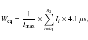
sampling time was 25 ns. The 32-channel filterbank and the
choice of
4.1
is the off-pulse
root-mean-square noise fluctuation. Pulses below the detection
threshold were discarded to ease storage requirements. The original
sampling time was 25 ns. The 32-channel filterbank and the
choice of
4.1 ![]() s
final time resolution resulted in 8192 phase bins. The time
resolution of 4.1
s
final time resolution resulted in 8192 phase bins. The time
resolution of 4.1 ![]() s
was chosen to match the estimated scattering
timescale available at the time (Sallmen
et al. 1999). However, it is known
from recent work by Bhat et al.
(2008) that single pulses at these radio
frequencies can be as narrow as 0.5
s
was chosen to match the estimated scattering
timescale available at the time (Sallmen
et al. 1999). However, it is known
from recent work by Bhat et al.
(2008) that single pulses at these radio
frequencies can be as narrow as 0.5 ![]() s. In addition to the single
pulses, average pulse profiles with 128 frequency channels in
each
20 MHz band were formed every 10 s.
s. In addition to the single
pulses, average pulse profiles with 128 frequency channels in
each
20 MHz band were formed every 10 s.
The reduced data consisted of ![]() 21 000 giant pulse candidates in
each recorded band. An example candidate is shown in Fig. 1,
where the pulse was detected in all bands. In the offline analysis
stage, these candidates were combined in software using only pulses
that show the expected dispersion delay. This method ensures that
spurious signals were filtered out in our analysis. After combining in
software, 12 959 giant pulses were identifed to have
occurred
simultaneously at all observed sky frequencies. Of the
12 959 pulses,
11384 were detected at the main pulse phase and 1370 at the interpulse
phase of the average pulse profile.
21 000 giant pulse candidates in
each recorded band. An example candidate is shown in Fig. 1,
where the pulse was detected in all bands. In the offline analysis
stage, these candidates were combined in software using only pulses
that show the expected dispersion delay. This method ensures that
spurious signals were filtered out in our analysis. After combining in
software, 12 959 giant pulses were identifed to have
occurred
simultaneously at all observed sky frequencies. Of the
12 959 pulses,
11384 were detected at the main pulse phase and 1370 at the interpulse
phase of the average pulse profile.
The data were folded and the single pulses were formed using
the DSPSR
software package and a polynomial determined by using TEMPO
(Taylor & Weisberg 1989).
The folded profiles formed in each 20-MHz band were
combined in software to validate the DM used. The combined data are
shown in Fig. 2
as a frequency-phase image and shows
no smearing, confirming that the value of DM is correct. A similar
procedure was used to combine simultaneous giant pulses in all seven
bands. Some artifacts of the 2-bit systems of the individual
telescopes are visible once the profile is summed for the entire
six-hour long observation. The width of these artifacts match the
dispersion smearing in the bands as seen in the top panel of
Fig. 2.
The quantisation noise is 12% for a single telescope,
whose signal is sampled using 2-bits (Cooper
1970). Since signals from
the 14 telescopes of the array were coherently summed, the
uncorrelated quantisation noise was reduced by a factor of ![]() .
The resulting noise of 3.7% is considered too small to
be problematic in the analysis that follows. In many stages of the
analysis, extensive use of the PSRCHIVE (Hotan
et al. 2004) utilities was
made to view and validate the pulsar data and to compute the S/N
used
in later analysis.
.
The resulting noise of 3.7% is considered too small to
be problematic in the analysis that follows. In many stages of the
analysis, extensive use of the PSRCHIVE (Hotan
et al. 2004) utilities was
made to view and validate the pulsar data and to compute the S/N
used
in later analysis.
![\begin{figure}
\par\includegraphics[width=8.5cm,clip]{13279fg1.ps}
\end{figure}](/articles/aa/full_html/2010/07/aa13729-09/img21.png)
|
Figure 1:
Total intensity of a coherently dedispersed giant pulse at the main
pulse phase detected in all recorded bands at 4.1 |
| Open with DEXTER | |
![\begin{figure}
\par\includegraphics[angle=-90,width=8cm,clip]{13279fg2.ps}
\end{figure}](/articles/aa/full_html/2010/07/aa13729-09/img22.png)
|
Figure 2: The plot shows the average pulse profile ( top panel) and the total intensity for six of the seven recorded bands in greyscale ( lower panel). The striped nature of channels at 1330 MHz and 1390 MHz comes from the overlap in the adajcent frequency bands. The roll-off of the filters used in the system is also seen as a reduced intensity at the band edges. A low-level extended feature is seen at the edge (also visible in the top panel as the elevated baseline in the right side of the main pulse) of each band which is due to the 2-bit quantisation noise and is only visible in long exposures. |
| Open with DEXTER | |
3 Flux calibration
![\begin{figure}
\par\includegraphics[angle=-90,width=8cm,clip]{13279fg3.ps}
\end{figure}](/articles/aa/full_html/2010/07/aa13729-09/img23.png)
|
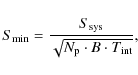
Figure 3:
The upper panel shows the change in minimum
detectable signal
|
| Open with DEXTER | |
where,
The term
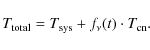
The peak flux of the giant pulses were computed using the
modified
radiometer equation (Lorimer &
Kramer 2005) for the pulsar case,
![]() .
With the above considerations of the
nebular contribution to
.
With the above considerations of the
nebular contribution to ![]() and with
and with ![]() K
in the
WSRT's L-Band, the system retained sufficiently
high sensitivity in
the first 15 000 s of the observation. Two other
factors have
been neglected in this calibration procedure and do not contribute
significantly to the
K
in the
WSRT's L-Band, the system retained sufficiently
high sensitivity in
the first 15 000 s of the observation. Two other
factors have
been neglected in this calibration procedure and do not contribute
significantly to the ![]() :
the relative change in the
orientation of the WSRT's fan beam and the Crab nebula over the course
of observation and the partial shadowing of three telescopes out of
the 14 for HA
:
the relative change in the
orientation of the WSRT's fan beam and the Crab nebula over the course
of observation and the partial shadowing of three telescopes out of
the 14 for HA ![]() (the last 3 h of our observation).
(the last 3 h of our observation).
4 Single-pulse statistics
For the analysis that follows, all pulses that were flux-calibrated as described in the previous section were used. The discussed change in system sensitivity does not limit this analysis thanks to our careful flux calibration procedure. While approximately 70% of the pulses were detected in all seven bands simultaneously, the rest were detected in two or more of the seven bands recorded. For the results described below, where applicable, only those pulses that were detected in all seven bands were used and explicitly mentioned.
4.1 Pulse intensity distributions
The giant pulse fluxes of the Crab pulsar contribute to the long
exponential tail of the single pulse intensity histograms
(Argyle & Gower 1972),
while the normal pulsars show Gaussian or exponential
pulse intensity distributions (Hesse
& Wielebinski 1974). Figure 4 shows the
average pulse flux distribution for pulses detected in at least two of
the seven recorded bands. The average pulse flux is computed by
integrating all emission within the equivalent width, ![]() of the
giant pulse (see Sect. 4.4).
This value is averaged over the pulse
period to obtain the average pulse flux. The pulse in each band was
detected based on a threshold of
of the
giant pulse (see Sect. 4.4).
This value is averaged over the pulse
period to obtain the average pulse flux. The pulse in each band was
detected based on a threshold of ![]() .
A pulse detected in two
bands satisfies the
.
A pulse detected in two
bands satisfies the ![]() limit. In the
first three hours of the observation (when the system was most
sensitive), the flux equivalent system noise in 4.1
limit. In the
first three hours of the observation (when the system was most
sensitive), the flux equivalent system noise in 4.1 ![]() s is
109 Jy. Averaged over the pulse period, a pulse of
s is
109 Jy. Averaged over the pulse period, a pulse of ![]() corresponds
to an average pulse flux density of 3.9 Jy. This implies
that it is sensitive to all pulses greater than
corresponds
to an average pulse flux density of 3.9 Jy. This implies
that it is sensitive to all pulses greater than ![]() ,
where
,
where ![]() mJy
is the average flux density
of the Crab pulsar. Therefore, the flux distribution computed here
contains a good fraction of weak giant pulses compared to those
reported elsewhere (see Table 2).
mJy
is the average flux density
of the Crab pulsar. Therefore, the flux distribution computed here
contains a good fraction of weak giant pulses compared to those
reported elsewhere (see Table 2).
The intensity distributions displayed in Fig. 4 shows at
least two components: a peak at or below ![]() 4 Jy - the weak
pulses that may comprise the trailing part of the normal pulse
distribution. The next component peaking at
4 Jy - the weak
pulses that may comprise the trailing part of the normal pulse
distribution. The next component peaking at ![]() 20 Jy resembles a
lognormal distribution with a power-law tail. The bright giant pulses
result in the extended power-law tail and is described by
20 Jy resembles a
lognormal distribution with a power-law tail. The bright giant pulses
result in the extended power-law tail and is described by ![]() ,
where NF
is the number of pulses detected in
1.8 Jy flux intervals of F. The value of
,
where NF
is the number of pulses detected in
1.8 Jy flux intervals of F. The value of ![]() and
and
![]() was determined from the best fits to the data in
the interval 118 Jy
was determined from the best fits to the data in
the interval 118 Jy
![]() Jy and
40 Jy
Jy and
40 Jy
![]() Jy
for the giant pulses in the main- and interpulse, respectively. Visual
inspection of Fig. 4
shows that the distribution is
multi-modal, with giant pulses in the region
Jy
for the giant pulses in the main- and interpulse, respectively. Visual
inspection of Fig. 4
shows that the distribution is
multi-modal, with giant pulses in the region ![]() Jy and the
pulses below this limit possibly representing normal pulses.
Jy and the
pulses below this limit possibly representing normal pulses.
![\begin{figure}
\par\includegraphics[angle=-90,width=8cm,clip]{13279fg4.ps}
\end{figure}](/articles/aa/full_html/2010/07/aa13729-09/img55.png)
|
Figure 4:
Distribution of the pulse intensity of all giant pulses detected at the
main- and interpulse phases in the upper and lower panels,
respectively. The long tail results from the giant pulse emission. The
best fit power-law curve is shown with slope |
| Open with DEXTER | |
Table 2: Reported sensitivity to the Crab giant pulse observations in the literature.
It is worth noting the differences in the intensity
distributions
displayed in Fig. 4.
While the distribution of the giant
pulses in the main pulse phase shows a clear turn over at ![]() 20 Jy,
the emergence of a bimodality in the region containing weak pulses is
evident in the intensity distribution of the interpulse giants. The
distribution corresponding to the interpulse phase also shows a
flattening in the 10-30 Jy region. The clear excess of weak
pulses in
both the distributions in the region
20 Jy,
the emergence of a bimodality in the region containing weak pulses is
evident in the intensity distribution of the interpulse giants. The
distribution corresponding to the interpulse phase also shows a
flattening in the 10-30 Jy region. The clear excess of weak
pulses in
both the distributions in the region ![]() Jy is due to our
method
of setting
Jy is due to our
method
of setting ![]() s (equal to
the time resolution). In this
case the emission window we considered is dominated by noise or weak
and narrow pulses. The slopes of the power-law models obtained here
can be compared to the values reported earlier. Figure 4 of
Lundgren et al. (1995)
shows a slope of
s (equal to
the time resolution). In this
case the emission window we considered is dominated by noise or weak
and narrow pulses. The slopes of the power-law models obtained here
can be compared to the values reported earlier. Figure 4 of
Lundgren et al. (1995)
shows a slope of ![]() for data at 800 MHz,
which is slightly steeper than the slopes of the main- and interpulse
distributions derived here. Cordes
et al. (2004) derive a value of
for data at 800 MHz,
which is slightly steeper than the slopes of the main- and interpulse
distributions derived here. Cordes
et al. (2004) derive a value of ![]() -2.3
at 433 MHz and Bhat
et al. (2008) found
-2.3
at 433 MHz and Bhat
et al. (2008) found ![]() at 1300 MHz,
which are comparable to the slope the main pulse intensity
distribution in our work. The slopes of the intensity distribution
reported here generally agree considering the effect of low number
statisics and/or dispersion smearing in the observations reported
elsewhere. While this experiment was sensitive to much lower fluxes,
the long observation time has also enabled the detection of rarer
bright pulses.
at 1300 MHz,
which are comparable to the slope the main pulse intensity
distribution in our work. The slopes of the intensity distribution
reported here generally agree considering the effect of low number
statisics and/or dispersion smearing in the observations reported
elsewhere. While this experiment was sensitive to much lower fluxes,
the long observation time has also enabled the detection of rarer
bright pulses.
4.2 Pulse energy distributions
![\begin{figure}
\par\includegraphics[angle=-90,width=8cm,clip]{13279fg5.ps}
\end{figure}](/articles/aa/full_html/2010/07/aa13729-09/img61.png)
|
Figure 5: The cumulative probablity distribution of the energy in giant pulses detected at the main pulse and the interpulse phases in the upper and lower panels, respectively. The y-axis is the fraction of the total number of pulses and pulse energy is plotted on the x-axis. Also shown are the occurrence rates per minute, second and hour. |
| Open with DEXTER | |
The relative occurrence rates of giant pulses is displayed as a
cumulative probablity distribution of the individual pulse energies in
Fig. 5.
The pulse energy is computed by multiplying the
equivalent width, ![]() ,
and the average pulse flux. As described
in Sect. 4.1,
we computed the best fits to the cumulative
probablity distributions of the main- and interpulse giants. The
power-law curve with
,
and the average pulse flux. As described
in Sect. 4.1,
we computed the best fits to the cumulative
probablity distributions of the main- and interpulse giants. The
power-law curve with ![]() and
and ![]() fits the data for pulse energies at the main- and inter pulse
phases, respectively. The break seen at
fits the data for pulse energies at the main- and inter pulse
phases, respectively. The break seen at ![]() 2000 Jy
2000 Jy ![]() s is
consistent with the break value reported by Popov
& Stappers (2007). The emission
at the interpulse phase shows a somewhat shallower power-law.
s is
consistent with the break value reported by Popov
& Stappers (2007). The emission
at the interpulse phase shows a somewhat shallower power-law.
It is known from Popov &
Stappers (2007) that the power-law index has a width
dependence, varying from -1.7 to -3.2 as the pulse width
increases. Based on this variation, the index we find is in good
agreement with Popov & Stappers
(2007) and Bhat
et al. (2008) (
![]() at 1300 MHz). However, we fit only a single power law
unlike the two power-law
fits found by these authors. Partial fits to the low-energy pulses
yield more than two components, with shallower power-law indices
indicating a simple dual-component fit is insufficient. One
explanation for this can be the bias introduced by setting
at 1300 MHz). However, we fit only a single power law
unlike the two power-law
fits found by these authors. Partial fits to the low-energy pulses
yield more than two components, with shallower power-law indices
indicating a simple dual-component fit is insufficient. One
explanation for this can be the bias introduced by setting
![]() s for narrow pulses,
overestimating the pulse
energy. However, this can only be a minor contribution and is an
argument that there is a clear break in the intensity distribution.
To compare the occurrence rates we see here, we proceed to derive the
rates from the arrival times of the giant pulses in the next section.
s for narrow pulses,
overestimating the pulse
energy. However, this can only be a minor contribution and is an
argument that there is a clear break in the intensity distribution.
To compare the occurrence rates we see here, we proceed to derive the
rates from the arrival times of the giant pulses in the next section.
4.3 Giant pulse rates
The distribution of the separation times between successive giant
pulses is plotted in Fig. 6. If the giant
pulses are
mutually exclusive events independent of each other, then the arrival
time separation follows a Poisson process (Lundgren
et al. 1995). The
probablity of a giant pulse occurring in the interval x
is then
given by ![]() ,
where
,
where ![]() is the mean pulse
rate. Since our data only consist of giant pulses, we expected to see
an exponential reduction in the separation time between the
pulses. Figure 6
shows the fits to the separation times
at both the inter- and main-pulse phases.
is the mean pulse
rate. Since our data only consist of giant pulses, we expected to see
an exponential reduction in the separation time between the
pulses. Figure 6
shows the fits to the separation times
at both the inter- and main-pulse phases.
![\begin{figure}
\par\includegraphics[angle=-90,width=8cm,clip]{13279fg6.ps}
\end{figure}](/articles/aa/full_html/2010/07/aa13729-09/img66.png)
|
Figure 6: The symbols show the distribution of separation times between successive giant pulses at the main- and interpulse phases and the solid lines are the best fits to the distribution. The top ordinate axis corresponds to the curve and data for the pulses at the main pulse phase and are offset by 450 for clarity. |
| Open with DEXTER | |
Functions with an exponential decay with time constants ![]() and
and ![]() are in excellent agreement
with the data at the main- and interpulse phases, respectively. From
the values of
are in excellent agreement
with the data at the main- and interpulse phases, respectively. From
the values of ![]() ,
the mean giant pulse rates are one main- pulse
giant every 0.9 s and one inter pulse giant every
5.81 s
observed above our threshold limit of 3.9 Jy. At these
frequencies,
the interpulse giants are comparatively less numerous as is evident
from our data. For comparision, the inter-pulse giants are brighter
and more frequent in frequency bands above 5.5 GHz (Cordes et al. 2004). The
combined rate of the giant pulses (fit and data not shown) is one
pulse every 0.803 s. The foregoing discussion confirms earlier
predictions that the giant pulse rate increases with frequency for the
Crab pulsar (Sallmen
et al. 1999; Lundgren et al. 1995). The
effect of the WSRT's
sensitivity reduction towards the end of the observation, as displayed
in Fig. 3,
may have contributed to the long tail of the
distribution, where fewer pulses were detected than in the first half
of the observation. However, the rate derived here is robust, since
the system had sufficiently high sensitivity in the first half of the
observation.
,
the mean giant pulse rates are one main- pulse
giant every 0.9 s and one inter pulse giant every
5.81 s
observed above our threshold limit of 3.9 Jy. At these
frequencies,
the interpulse giants are comparatively less numerous as is evident
from our data. For comparision, the inter-pulse giants are brighter
and more frequent in frequency bands above 5.5 GHz (Cordes et al. 2004). The
combined rate of the giant pulses (fit and data not shown) is one
pulse every 0.803 s. The foregoing discussion confirms earlier
predictions that the giant pulse rate increases with frequency for the
Crab pulsar (Sallmen
et al. 1999; Lundgren et al. 1995). The
effect of the WSRT's
sensitivity reduction towards the end of the observation, as displayed
in Fig. 3,
may have contributed to the long tail of the
distribution, where fewer pulses were detected than in the first half
of the observation. However, the rate derived here is robust, since
the system had sufficiently high sensitivity in the first half of the
observation.
4.4 Width distributions
The equivalent pulse width, ![]() is defined as the width of a
top-hat pulse with height equal to the peak intensity of the
pulse.
is defined as the width of a
top-hat pulse with height equal to the peak intensity of the
pulse. ![]() for the giant pulses detected in all seven bands was
computed. The results are displayed in panels on the right in
Fig. 7.
We express
for the giant pulses detected in all seven bands was
computed. The results are displayed in panels on the right in
Fig. 7.
We express ![]() as
as
where
![\begin{figure}
\par\includegraphics[angle=-90,width=8.5cm,clip,clip]{13279fg7.ps}
\end{figure}](/articles/aa/full_html/2010/07/aa13729-09/img73.png)
|
Figure 7:
Plot of intensity against pulse width for the main- and interpulse
windows in the top left and lower left panels.
Histograms of equivalent pulse widths are shown in the top
right and lower right panels. The distribution has an
exponential envelope. For pulses with computed |
| Open with DEXTER | |
The giant pulses at these frequencies can be quite narrow. For
instance, Bhat et al. (2008)
find pulse widths to be 0.5 ![]() s and
Eilek et al. (2002)
found 0.2
s and
Eilek et al. (2002)
found 0.2 ![]() s.
Our method of data reduction allowed
a time resolution of 4.1
s.
Our method of data reduction allowed
a time resolution of 4.1 ![]() s, so pulses with
s, so pulses with ![]() s
were taken to have a width equal to 4.1
s
were taken to have a width equal to 4.1 ![]() s. This results in some
pulses being underestimated in flux and overestimated in equivalent
width. The computed equivalent widths range from 4.1
s. This results in some
pulses being underestimated in flux and overestimated in equivalent
width. The computed equivalent widths range from 4.1 ![]() s to
s to
![]() 120
120 ![]() s, and we
find that bright pulses tend to be narrow
as seen in the left hand panels of Fig. 7. This was also
suggested by Sallmen et al.
(1999) and shown by Eilek
et al. (2002). Popov
& Stappers (2007)
found a similar behaviour in addition to a width-dependent break in
the power-law fits to the pulse-energy distribution.
s, and we
find that bright pulses tend to be narrow
as seen in the left hand panels of Fig. 7. This was also
suggested by Sallmen et al.
(1999) and shown by Eilek
et al. (2002). Popov
& Stappers (2007)
found a similar behaviour in addition to a width-dependent break in
the power-law fits to the pulse-energy distribution.
In the seven closely spaced radio bands observed, we note that
a vast
majority of the pulses have widths larger than 4.1 ![]() s. This is
seen in the pulse width histograms at the two pulse phases, displayed
in the panels on the right in Fig. 7. The distribution
shows
a peak at
s. This is
seen in the pulse width histograms at the two pulse phases, displayed
in the panels on the right in Fig. 7. The distribution
shows
a peak at ![]() 16
16![]() s, which
is 4 times our ultimate time
resolution in the main pulse, and the peak shifts towards narrower
timescales for the interpulses. We find less than
s, which
is 4 times our ultimate time
resolution in the main pulse, and the peak shifts towards narrower
timescales for the interpulses. We find less than ![]() of the pulses
with
of the pulses
with ![]() s,
indicating that the majority of the pulses
show wider widths than our time resolution. The shape of the width
distribution is similar at both the main- and interpulse phases.The
contribution to the tail region of the distribution comes from scatter
broadened pulses.
s,
indicating that the majority of the pulses
show wider widths than our time resolution. The shape of the width
distribution is similar at both the main- and interpulse phases.The
contribution to the tail region of the distribution comes from scatter
broadened pulses.
4.5 Spectral index of giant pulses
The data were recorded in 7 different radio bands each 20 MHz
wide in
the frequency range 1300-1450 MHz, and several thousands of
pulses
were detected simultaneously in all bands. The spectral index of
individual pulses was computed by modelling the flux variation of a
giant pulse as ![]() .
Here,
.
Here, ![]() is the flux of
the giant pulse at frequency
is the flux of
the giant pulse at frequency ![]() ,
and k the spectral index. The
histograms of the derived spectral indices are displayed in
Fig. 8
for the giants at both pulse phases. A large
dispersion in the spectral index is seen, with values
,
and k the spectral index. The
histograms of the derived spectral indices are displayed in
Fig. 8
for the giants at both pulse phases. A large
dispersion in the spectral index is seen, with values ![]() for the
main- and
for the
main- and ![]() for the interpulse giants.
for the interpulse giants.
![\begin{figure}
\par\includegraphics[angle=-90,width=8cm,clip]{13279fg8.ps}
\end{figure}](/articles/aa/full_html/2010/07/aa13729-09/img80.png)
|
Figure 8: Histogram of spectral indices for the giant pulses detected at the main pulse ( bottom panel) and the interpulse phase ( top panel). The spread in the distributions is indicative of fitting errors. See text for details. |
| Open with DEXTER | |
These spectral index values are quite a bit shallower than those
detected previously (see Introduction) over wider frequency
separations. We therefore consider the effects of diffractive
interstellar scintillation (DISS) on the spectral index
estimates. Strong DISS results in pulse intensity variations within
each of the seven bands. The effect of scintillation is to modulate
the observed pulsar signal in both time and frequency. This is seen as
regions of enhanced or diminished brightness in a grey scale plot of
the intensity as a function of time and frequency. These regions are
known as scintles. We estimate the scintillation bandwidth based on
the pulse scatter timescales, ![]() s
at sky
frequency of 200 MHz, as reported in the work of Bhat et al. (2007). We
further make use of their revised
s
at sky
frequency of 200 MHz, as reported in the work of Bhat et al. (2007). We
further make use of their revised ![]() frequency
scaling and consider that the scintillation bandwidth and
scattering timescale are related by
frequency
scaling and consider that the scintillation bandwidth and
scattering timescale are related by ![]() ,
where the constant C1=1.05
for a thin scattering screen
(Cordes et al. 2004).
From these considerations
,
where the constant C1=1.05
for a thin scattering screen
(Cordes et al. 2004).
From these considerations ![]() MHz
in the 1300-1460 MHz band. On examining a few giant
pulses by eye, it was clear that some of the scintles are resolved,
while some were narrower than our channel width of
MHz
in the 1300-1460 MHz band. On examining a few giant
pulses by eye, it was clear that some of the scintles are resolved,
while some were narrower than our channel width of ![]() MHz.
Thus, in the flux obtained by integrating the signal in the
20 MHz-wide bands, the scintles tend to average out. This
implies that
scintillation does not cause the spread in the individual giant-pulse
spectral indices. Moreover, with such narrow
scintillation bandwidths, averaging over many giant pulse spectral
index determinations as we have done here would give an average
spectral index that reflects the true average spectral index.
MHz.
Thus, in the flux obtained by integrating the signal in the
20 MHz-wide bands, the scintles tend to average out. This
implies that
scintillation does not cause the spread in the individual giant-pulse
spectral indices. Moreover, with such narrow
scintillation bandwidths, averaging over many giant pulse spectral
index determinations as we have done here would give an average
spectral index that reflects the true average spectral index.
Refractive interstellar scintillation (RISS) cannot corrugate
the
spectra of single pulses, since the pulse intensity variations due to
RISS are noticeable in observation of the order of a few days
(Lundgren et al. 1995).
However, the pulses do have a significant structure
that is intrinsic to the emission process. One example is displayed in
Fig. 1
and these pulses do contribute to the spread in the
computed spectral indices. In this figure, it is clear that the
leading short burst shows considerable variation across the seven
bands, while the scattered trailing part of the pulse is correlated
across frequency. This is again similar to what Hankins
& Eilek (2007) find, as
shown in their Fig. 4, but at a much higher frequency of ![]() 9 GHz.
9 GHz.
Sallmen et al. (1999)
find that the spectral index variation is between
-4.9 and -2.2 based on 29 pulses they observed in two bands
centred at 1.4 GHz and 0.6 GHz. The spread in the
indices computed
here and that of Sallmen
et al. (1999) points to the stochastic nature of the
giant pulse emission process and/or the disturbed plasma flow in the
magnetosphere caused by strong plasma turbulence (Hankins
& Eilek 2007). The
giant pulses used in this analysis were detected in all seven bands
and represent 70![]() of all detected pulses in our data. Since each of
our bands is 20 MHz wide, detection in seven bands implies an
emission
bandwidth of at least
of all detected pulses in our data. Since each of
our bands is 20 MHz wide, detection in seven bands implies an
emission
bandwidth of at least ![]() MHz.
This suggests that the
emission bandwidth of Crab giant pulses is potentially greater than
MHz.
This suggests that the
emission bandwidth of Crab giant pulses is potentially greater than
![]() ,
unlike the giant pulse emission from the
millisecond pulsar B1937+21 (Popov
& Stappers 2003). We note that the
,
unlike the giant pulse emission from the
millisecond pulsar B1937+21 (Popov
& Stappers 2003). We note that the
![]() for the Crab giant pulses reported by
Sallmen et al. (1999)
was based on 29 simultaneous giant pulses from their
90-min observation (
for the Crab giant pulses reported by
Sallmen et al. (1999)
was based on 29 simultaneous giant pulses from their
90-min observation (![]() 161 086 stellar
rotations). Those 29 pulses could have been chance detections,
while the
161 086 stellar
rotations). Those 29 pulses could have been chance detections,
while the ![]() limit derived here comes from a much larger sample of giant
pulses so is more robust. We detected a total of
17 587 giant
pulses, of which approximately 4000 were detected in less than
7 bands. Clearly it is impossible to include the pulses
detected in only
a few bands in this analysis as that would increase the dispersion in
the spectral indices computed; however, this lack of detection in all
bands, for pulses which were clearly detected in the other bands, is
an argument for there being some narrow band effects that appear to
modulate the giant pulse intensity.
limit derived here comes from a much larger sample of giant
pulses so is more robust. We detected a total of
17 587 giant
pulses, of which approximately 4000 were detected in less than
7 bands. Clearly it is impossible to include the pulses
detected in only
a few bands in this analysis as that would increase the dispersion in
the spectral indices computed; however, this lack of detection in all
bands, for pulses which were clearly detected in the other bands, is
an argument for there being some narrow band effects that appear to
modulate the giant pulse intensity.
5 Double giant pulses
During direct inspection of some giant pulses, it was noticed that
occasional giant pulse emission was evident at both the main- and
interpulse phases within a single rotation period of the star. To
determine how many such pulses were present, the following search
algorithm was used. First, the giant pulses detected in all seven
bands were combined in software across the frequency bands. The pulses
were then averaged over polarisation and frequency to create single
pulse total intensity profiles. The search algorithm was made
sensitive to emission at both emission windows (main- and interpulse)
by traversing each pulse profile twice; in the first pass, the
emission peak and phase information was recorded, following which a
search is made in the other emission window i.e. if a pulse was
detected at the main pulse phase we check whether a pulse is also seen
at the interpulse phase. All pulses that show signal ![]()
![]() in
the second emission window are collected separately. The pulses
returned by the search procedure were examined by eye to validate the
double pulse nature. To our knowledge, this is the first instance of
this phenomena being reported. A total of 197 pulses
that show
emission at both pulse phases were found in our data set above the
in
the second emission window are collected separately. The pulses
returned by the search procedure were examined by eye to validate the
double pulse nature. To our knowledge, this is the first instance of
this phenomena being reported. A total of 197 pulses
that show
emission at both pulse phases were found in our data set above the
![]() detection
threshold.
detection
threshold.
![\begin{figure}
\par\includegraphics[angle=-90,width=8cm,clip]{13279fg9.ps}
\end{figure}](/articles/aa/full_html/2010/07/aa13729-09/img92.png)
|
Figure 9: Detected double giant pulses shown as a ratio of the main pulse to the interpulse flux. The x-axis shows time since the start of the observation. |
| Open with DEXTER | |
To consider how likely this is to happen by chance, we note that the
observation lasted 643 263 rotations of the star and
11 584 and 1375 giant pulses were found at the main-
and interpulse phases,
respectively, above the ![]() detection threshold in each
band. Since these giant pulses were detected in all seven bands, the
effective threshold is now
detection threshold in each
band. Since these giant pulses were detected in all seven bands, the
effective threshold is now ![]() .
If the
.
If the
![]() criterion is
used to search for the double pulses, a total
of 17 pulses are seen. In other words, only 17 pulses in the
197 detected show
criterion is
used to search for the double pulses, a total
of 17 pulses are seen. In other words, only 17 pulses in the
197 detected show ![]() in either of the two emission
windows. Let the giant pulses occurring at the two pulse phases be
independent events, with individual probablitites P(A)
and
P(B). The chance of two giant
pulses occurring within a single
rotation period is the joint probablity P(A,B)=P(A).P(B).
Thus the
chance of detecting a giant pulse above the
in either of the two emission
windows. Let the giant pulses occurring at the two pulse phases be
independent events, with individual probablitites P(A)
and
P(B). The chance of two giant
pulses occurring within a single
rotation period is the joint probablity P(A,B)=P(A).P(B).
Thus the
chance of detecting a giant pulse above the ![]() threshold limit
at the main- and interpulse phases are P(A)=11584/643263
and P(B)=
1375/642 263 leading to
threshold limit
at the main- and interpulse phases are P(A)=11584/643263
and P(B)=
1375/642 263 leading to ![]() .
We therefore
expect a total of
.
We therefore
expect a total of ![]() pulse
periods with pulses
at both phases in our data. The detection of 17 pulses is thus
consistent with the expected 24 pulses.
pulse
periods with pulses
at both phases in our data. The detection of 17 pulses is thus
consistent with the expected 24 pulses.
As seen above, combining the seven bands improves sensitivity
and
allows the detection of weaker pulses. Considering pulses with S/Ngreater
than ![]() in the second emission window resulted in the
detection of an additional 180 double pulses. While the 197 pulses
detected are not sufficient to perform meaningful statistics of these
pulses, in Sect. 6.1
we use our population of double giant
pulses to study scintillation and scattering within a 0.5 rotation of
the pulsar.
in the second emission window resulted in the
detection of an additional 180 double pulses. While the 197 pulses
detected are not sufficient to perform meaningful statistics of these
pulses, in Sect. 6.1
we use our population of double giant
pulses to study scintillation and scattering within a 0.5 rotation of
the pulsar.
Although the appearance of the pulses in the same rotation
period is
consistent with the individual occurrence rates, we compared the GP
properties at each phase. In the double pulses, the emission in the
interpulse phase is typically narrower (
![]() s)
than
the emission at the main pulse phase and pulses at the main pulse
phase are typically brighter, as shown in Fig. 9. In
both cases this is consistent with the known population of GPs at each
phase. A similar analysis to the one in Sect. 4.3 was done to
determine the rate of double pulses and a rate
of 1 pulse in 84 s, or one in
2545 rotations of the star was found to have giant
pulse emission at both pulse phases. Thus, given the narrowness and
very low occurrence rates of these pulses, they were easily missed in
earlier observations.
s)
than
the emission at the main pulse phase and pulses at the main pulse
phase are typically brighter, as shown in Fig. 9. In
both cases this is consistent with the known population of GPs at each
phase. A similar analysis to the one in Sect. 4.3 was done to
determine the rate of double pulses and a rate
of 1 pulse in 84 s, or one in
2545 rotations of the star was found to have giant
pulse emission at both pulse phases. Thus, given the narrowness and
very low occurrence rates of these pulses, they were easily missed in
earlier observations.
6 Single-pulse scattering
The frequency resolution and large bandwidth of our data benefits
scattering and scintillation checks on the individual pulses in two
ways. First, the pulses detected in 7 bands are combined in software
to give 224 channels across the 140 MHz bandwidth allowing
examination
of scintillation. Second, the large bandwidth of the combined pulse
increases sensitivity and makes it possible to identify low-level
extended scatter tails. To characterise the scattering time ![]() in the
pulsar signal, we computed the extent of pulse broadening in
the individual giant pulses. If the pulses are scattered by a
thin-screen between the source and the observer, the pulses can then
be modelled as an one-sided exponential with a vertical rise and a
rapid decay (Williamson 1972).
This can be written as
in the
pulsar signal, we computed the extent of pulse broadening in
the individual giant pulses. If the pulses are scattered by a
thin-screen between the source and the observer, the pulses can then
be modelled as an one-sided exponential with a vertical rise and a
rapid decay (Williamson 1972).
This can be written as
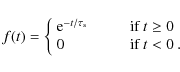
This model was fit to the data using a least-squares minimisation and the 1/e time derived from the models was taken as
![\begin{figure}
\par\includegraphics[angle=-90,width=7.8cm,clip]{13279fg10.ps}
\end{figure}](/articles/aa/full_html/2010/07/aa13729-09/img102.png)
|
Figure 10:
Upper panel: a plot of the values of time
constant |
| Open with DEXTER | |
The lower panel of Fig. 10
shows an exponential
envelope in the distribution of ![]() .
The individual pulse
scattering time varies from 4.1
.
The individual pulse
scattering time varies from 4.1 ![]() s to
s to ![]() 90
90![]() s. The large
number of pulses in the distribution with
s. The large
number of pulses in the distribution with ![]() s
is
related to our ultimate time resolution of 4.1
s
is
related to our ultimate time resolution of 4.1 ![]() s. This also
implies that a large fraction of the pulses have scattering time
s. This also
implies that a large fraction of the pulses have scattering time
![]() s.
At a slightly earlier epoch than our
observations, Bhat et al.
(2007) determined a value of
s.
At a slightly earlier epoch than our
observations, Bhat et al.
(2007) determined a value of ![]() s
at 200 MHz. Using their revised frequency scaling of
s
at 200 MHz. Using their revised frequency scaling of
![]() ,
the scattering time at the centre
of our band (1373 MHz) is
,
the scattering time at the centre
of our band (1373 MHz) is ![]() s. At a
slightly later
epoch, Bhat et al. (2008)
find a value of
s. At a
slightly later
epoch, Bhat et al. (2008)
find a value of ![]() s
at 1300 MHz, which contrasts with the value of
8 ms at 111 MHz (or 1.4
s
at 1300 MHz, which contrasts with the value of
8 ms at 111 MHz (or 1.4 ![]() s at
1300 MHz using a
s at
1300 MHz using a ![]() scaling law) reported by
Kuzmin et al. (2008).
With our data, we are not sensitive to scatter times
below 4.1
scaling law) reported by
Kuzmin et al. (2008).
With our data, we are not sensitive to scatter times
below 4.1 ![]() s,
but to the dispersion seen in the histogram of
scatter times in Fig. 10
shows that variations can even
be expected within a single observation of six hours. We again refer
to Fig. 1
for an example of the extreme form of this
variation: the different parts of the same pulse
show different
scattering effects, imparting a significant structure to the pulse. In
their work on DISS, Cordes &
Rickett (1998) emphasise that considering the 1/etime
equal to
s,
but to the dispersion seen in the histogram of
scatter times in Fig. 10
shows that variations can even
be expected within a single observation of six hours. We again refer
to Fig. 1
for an example of the extreme form of this
variation: the different parts of the same pulse
show different
scattering effects, imparting a significant structure to the pulse. In
their work on DISS, Cordes &
Rickett (1998) emphasise that considering the 1/etime
equal to
![]() is only valid for a thin screen and does not
always hold. In light of the limited validity in interpreting the
1/e time and the spread in the values of scatter
times found in our
analysis, we suggest that the scattering in the direction of Crab
pulsar cannot be modelled by single thin screen. The spread in
is only valid for a thin screen and does not
always hold. In light of the limited validity in interpreting the
1/e time and the spread in the values of scatter
times found in our
analysis, we suggest that the scattering in the direction of Crab
pulsar cannot be modelled by single thin screen. The spread in
![]() ranges from
ranges from ![]()
![]() s to
s to ![]()
![]() s in our
s in our ![]() 6 hour-observation.
This proves most of the scattering cannot be due to
the ISM, as the line of sight through the ISM does not change rapidly
enough to explain these variations. Therefore, the bulk of scattering
should orginate in the Crab nebula. The nebula can clearly give rise
to a complex screen or changes in the structures in the vicinity of
the pulsar that give rise to the short-term changes in scattering time
(Sallmen
et al. 1999; Lyne et al. 2001; Backer
et al. 2000). The scattering of pulses cannot be in
the
pulsar magnetosphere. In that case the pulses at lower frequencies
that originate higher up in the magnetosphere should show lower
scatter times, because according to the standard pulsar models, the
number density of charged particles is lower in the upper
magnetosphere (Lyubarskii &
Petrova 1998). However,
6 hour-observation.
This proves most of the scattering cannot be due to
the ISM, as the line of sight through the ISM does not change rapidly
enough to explain these variations. Therefore, the bulk of scattering
should orginate in the Crab nebula. The nebula can clearly give rise
to a complex screen or changes in the structures in the vicinity of
the pulsar that give rise to the short-term changes in scattering time
(Sallmen
et al. 1999; Lyne et al. 2001; Backer
et al. 2000). The scattering of pulses cannot be in
the
pulsar magnetosphere. In that case the pulses at lower frequencies
that originate higher up in the magnetosphere should show lower
scatter times, because according to the standard pulsar models, the
number density of charged particles is lower in the upper
magnetosphere (Lyubarskii &
Petrova 1998). However, ![]() scales with frequency as
scales with frequency as
![]() (Popov et al. 2006),
and this does not support the hypothesis
that scattering could have its orgins in the pulsar magnetosphere.
(Popov et al. 2006),
and this does not support the hypothesis
that scattering could have its orgins in the pulsar magnetosphere.
The diffractive scintillation timescale, ![]() at this
frequency was estimated by Cordes
et al. (2004) as 25.5 s, based on pairs of
single pulses with sufficient S/N.
However, the pulse pairs they
used were separated in time by a few pulse periods. Since our data has
good frequency resolution (224 frequency channels across
140 MHz), and
we detected several pulses with multiple components, we proceeded to
estimate possible variations in the scintillation time on shorter
timescales.
at this
frequency was estimated by Cordes
et al. (2004) as 25.5 s, based on pairs of
single pulses with sufficient S/N.
However, the pulse pairs they
used were separated in time by a few pulse periods. Since our data has
good frequency resolution (224 frequency channels across
140 MHz), and
we detected several pulses with multiple components, we proceeded to
estimate possible variations in the scintillation time on shorter
timescales.
6.1 Scintillation within single pulses
The scintillation timescale within single pulses was estimated using
those pulses that show well separated components and the double pulses
discussed in Sect. 5.
The search for at least two
components in single pulses was carried out based on the component
separation of ![]() 25
25![]() s. This was
done by examining the pulses
by eye, after an automated first pass. The first pass provided 451
giant pulse candidates, 368 of those displayed at least two distinct
shots in the main pulse phase, and 18 candidates were found in the
interpulse phase. The 197 double pulses were included in this
analysis. Assuming that the two shots of pulses are intrinsic to the
pulsar emission and that the scattering screen remains stable within a
pulse period, any scintillation would affect the two components
similarly, introducing a correlated frequency structure. The
scintillation timescale is then the 1/e point along
the time axis of
the 2-dimensional intensity correlation function,
s. This was
done by examining the pulses
by eye, after an automated first pass. The first pass provided 451
giant pulse candidates, 368 of those displayed at least two distinct
shots in the main pulse phase, and 18 candidates were found in the
interpulse phase. The 197 double pulses were included in this
analysis. Assuming that the two shots of pulses are intrinsic to the
pulsar emission and that the scattering screen remains stable within a
pulse period, any scintillation would affect the two components
similarly, introducing a correlated frequency structure. The
scintillation timescale is then the 1/e point along
the time axis of
the 2-dimensional intensity correlation function, ![]() of the spectrum
(Cordes 1986). The computed
correlation coefficients between the two
components and the double pulses are displayed in
Fig. 11.
of the spectrum
(Cordes 1986). The computed
correlation coefficients between the two
components and the double pulses are displayed in
Fig. 11.
![\begin{figure}
\par\includegraphics[angle=-90,width=7.8cm,clip]{13279fg11.ps}
\end{figure}](/articles/aa/full_html/2010/07/aa13729-09/img113.png)
|
Figure 11:
Correlation coefficients of the spectra within a single pulse period.
Top panel shows correlation between the two components of
giant pulse, while lower panel is the double
giants. The separation between the components |
| Open with DEXTER | |
The correlation coefficient of ![]() 0.4 for many pulse component
pairs is in excellent agreement with the value derived by
Cordes et al. (2004).
They derive a value of 0.33 considering the giant
pulses to be 100% polarised, amplitude modulated, scintillated shot
noise. It also implies that these components have undergone similar
scintillation effects, ruling out the possibility of any variation in
the scattering medium on these timescales. The average correlation
coefficients computed for the double pulses is consistent with the
average value computed for the widely spaced pulse components (pulses
in the top panel of Fig. 11).
Since a clear roll-off in the
values of correlation coefficient is not seen in the data presented
here, we conclude that the scintillation timescales are longer
than 14 ms, which is entirely consistent with Cordes et al. (2004).
0.4 for many pulse component
pairs is in excellent agreement with the value derived by
Cordes et al. (2004).
They derive a value of 0.33 considering the giant
pulses to be 100% polarised, amplitude modulated, scintillated shot
noise. It also implies that these components have undergone similar
scintillation effects, ruling out the possibility of any variation in
the scattering medium on these timescales. The average correlation
coefficients computed for the double pulses is consistent with the
average value computed for the widely spaced pulse components (pulses
in the top panel of Fig. 11).
Since a clear roll-off in the
values of correlation coefficient is not seen in the data presented
here, we conclude that the scintillation timescales are longer
than 14 ms, which is entirely consistent with Cordes et al. (2004).
7 Discussion
To our knowledge this is the largest collection of high time-resolution giant pulse analysis presented in the literature. Even though some features of the giant pulse emission like the giant nano shots are in the process of being explained (Hankins & Eilek 2007), several questions still remain about the pulsar emission mechanism in general and the giant pulse phenomena in particular. From the measured pulse widths and the observed structure in many pulses, it is evident from the analysis presented in this paper that the giant pulse emission is a manifestation of temporal plasma changes in the pulsar magnetosphere. The observed giant pulse rates are further evidence for this temporal variation, because if the mechanism responsible for the giant pulses is active on timescales longer than a pulse period, a clear excess of giant pulses separated by a single rotation period can be expected. On the basis of the giant pulse arrival times, it was concluded that the observed giant pulse emission does not come from a steady emission beam loosely bound to the stellar surface (Sallmen et al. 1999; Lundgren et al. 1995). We confirm that our data do not support such a model, for if such a beam with random wobbles operates, a characteristic width in the giant pulses can be expected. In other words, the distribution of the pulse widths would be normally distributed with a mean width.
The power-law nature of the giant pulse intensity distributions was shown by Lundgren et al. (1995), and they inferred that the normal pulses formed a separate part of the intensity distributions. In this work, we have shown conclusively that the giant pulses consist of two distinct populations especially for those pulses found at the inter pulse phase. We see a definite change in the shape of the distribution of pulse energies as we go to lower energies and we also see a slight broadening of the pulses. These pulses still seem to be distinct from what might be called ``normal pulses'': they are still narrower than most subpulses and are at least 27 times brighter than the normal pulses. The slope of the distribution containing these pulses is different from rest of the intensity distribution. These pulses could possibly be the trailing part of the distribution inferred by Lundgren et al. (1995). Moreover, how these relate to the precursor emission is unclear, which can clearly be improved upon using the double giant pulses. While there is evidence of a broadening of the pulses as they weaken in intensity, they do not appear to be as broad as standard subpulses. This finding has implications in the model derived by Petrova (2004), where a clear power-law distribution is explained, but not a weak giant population. The power-law index derived also has implications for interpreting giant pulse emission on the basis of self organised criticality (Bak et al. 1987), as suggested by Cairns (2004).
The spectral index of the Crab giant pulses reported in this
work
suggests that the emission bandwidth is at least ![]() and
may approach the upper limit
and
may approach the upper limit ![]() predicted in
numerical models by Weatherall (1998).
Hankins & Eilek (2007)
find a similar
emission bandwidth at 9.5 GHz. Moreover, the average spectral
index of
giant pulses at the interpulse phase is flatter than the giant pulses
at the main pulse phase. This possibly explains the dominant and
bright nature of interpulse giants at
predicted in
numerical models by Weatherall (1998).
Hankins & Eilek (2007)
find a similar
emission bandwidth at 9.5 GHz. Moreover, the average spectral
index of
giant pulses at the interpulse phase is flatter than the giant pulses
at the main pulse phase. This possibly explains the dominant and
bright nature of interpulse giants at ![]() GHz. We note the
prominent emergence of bimodality in the intensity distribution of the
interpulses relative to the main phase pulses. Furthermore,
(Hankins & Eilek 2007)
find upward drifting emission bands in the spectrum of
the interpulses giants and not in the main pulse giants. These
differences strongly suggest a different nature to the interpulses. To
explain the drifting emission bands, Lyutikov
(2007) derived an excess
plasma density of
GHz. We note the
prominent emergence of bimodality in the intensity distribution of the
interpulses relative to the main phase pulses. Furthermore,
(Hankins & Eilek 2007)
find upward drifting emission bands in the spectrum of
the interpulses giants and not in the main pulse giants. These
differences strongly suggest a different nature to the interpulses. To
explain the drifting emission bands, Lyutikov
(2007) derived an excess
plasma density of ![]() 105
and a large Lorentz factor of the
emitting particles of the order of
105
and a large Lorentz factor of the
emitting particles of the order of ![]() 107, and this condition is
satisfied close to the light cylinder over the magnetic
equator. However, the model proposed by Lyutikov
(2007) is only valid
for
107, and this condition is
satisfied close to the light cylinder over the magnetic
equator. However, the model proposed by Lyutikov
(2007) is only valid
for ![]() GHz,
where the emission bands are observed. While
results from our observations can neither support nor rule out this
model, the difference in pulse intensity distributions we find
indicates that the interpulse giants are different in nature.
GHz,
where the emission bands are observed. While
results from our observations can neither support nor rule out this
model, the difference in pulse intensity distributions we find
indicates that the interpulse giants are different in nature.
It is worth noting that the pulsar signal is a stochastic process that contributes to the measurement noise of the pulsed intensity. This is especially true in the case of giant pulse emission, where pulsed flux can exceed 1500 Jy, an order of magnitude greater than the system equivalent flux density (SEFD) of approximately 145 Jy. Source-intrinsic noise increases the measurement uncertainty of various derived parameters, such as the pulsed flux density, pulse width, scattering time, and spectral index van Straten (2009). In addition, any temporal and/or spectral correlations - either intrinsic to the giant pulse emission or induced by interstellar scintillation - will also affect the uncertainties of any derived parameters. The vast majority of the pulses presented in this analysis have average flux densities that are lower than the SEFD, and we do not expect that self-noise will significantly alter the results of this analysis. To accurately quantify the impact of self-noise on parameter distributions (such as those presented in Figs. 4, 5, 7, and 8) would require extensive simulations that are beyond the scope of the present work but may provide additional insight in a future paper.
The previously unreported double pulses we found are consistent with the occurrence rate on a purely probabilistic basis. Collecting even more of these pulse pairs would allow for better checks of the statistics of occurrence to ascertain that they are chance occurrences and not indicative of some longer term underlying phenomenon driving the giant pulse emisision. Moreover detecting more of these pulses at higher time resolution would provide further insight into the nature of these pulses. Hankins & Eilek (2007) found that the giant pulses at the interpulse phase show an additional dispersion when compared to the pulses at the main pulse phase. The closest pulse pair they were able to examine were separated by 12 min. One may gain new insight into the excess dispersion seen at the interpulse phase by examining the double giant pulses, which are the closest giant pulse pair possible.
Scattering analysis of single pulses presented in this paper
show a
variety of scattering times and corroborates with the analysis of
Sallmen et al. (1999).
They show that scattering from multiple screens or a
single thick screen is excluded because of the observed frequency
independence of the pulse component separation. From this it was
concluded that the multiple components that make up the giant pulses
are intrinisic to the emission mechanism. Using multiple components
and the double pulses, we conclude that the scintillation timescales
are greater than 14 ms, which indicates that there are no
large
changes in the number density of the scattering medium along the line
of sight through the nebula on similar timescales. That the multiple
components we detect in the giant pulses are spaced by at least
25 ![]() s
implies that the magnetosphere and/or the plasma does not
change on these timescales, if the source intrinsic emission is less
than 25
s
implies that the magnetosphere and/or the plasma does not
change on these timescales, if the source intrinsic emission is less
than 25 ![]() s.
On the other hand, giant pulses may consist of
overlapping nano shots. In this case the competing models make use of
plasma turbulence leading to modulational instablity (Weatherall 1998) or
the induced Compton scattering of low-frequency radio waves
(Petrova 2004) in the
magnetosphere to explain the origin of the nano
shots. While with our data we are not sensitive to the pulses less
than 4.1
s.
On the other hand, giant pulses may consist of
overlapping nano shots. In this case the competing models make use of
plasma turbulence leading to modulational instablity (Weatherall 1998) or
the induced Compton scattering of low-frequency radio waves
(Petrova 2004) in the
magnetosphere to explain the origin of the nano
shots. While with our data we are not sensitive to the pulses less
than 4.1 ![]() s
duration, there is an indication that the emission
bandwidth
s
duration, there is an indication that the emission
bandwidth ![]() ,
suggesting that the pulses can
potentially have structure as narrow as 3.6 ns at this
frequency.
,
suggesting that the pulses can
potentially have structure as narrow as 3.6 ns at this
frequency.
8 Conclusions
The large collection of single pulses we gathered has allowed us to perform a range of statistics with the data. After careful flux calibration, a detailed analysis of the pulse intensities, energies, widths, and separation times was done by computing distributions of these quantities. In the single-pulse intensity distributions, we find a clear evidence of two distinct populations in the giant pulses. The giant pulse separation times show a Poission distribution, and the rate of occurrence of giant pulses was determined. Spectral indices for a large number of giant pulses were computed with the narrowly spaced multi band data. Significant dispersion in the spectral indices was found and a small negative average spectral index was found for the main- and interpulse giants, and they are flatter than the average pulse emission. We also note that in some cases there is evidence for intensity modulation with bandwidths that are smaller than the full band but not consistent with scintillation effects. The previously undetected double giant pulses were presented and we find that they are not more frequent than would be expected by chance. The scatter time for a large number of giant pulses was determined by modelling the scatter broadening as an exponenial function and the distribution of scatter times was computed. The double giant pulses were reported for the first time and it is found that they are not very different from the normal giant pulses. Using multiple emission components either at the main- or interpulse phase and the double giant pulses, we find no evidence of variation of the scattering material on timescales shorter than 14 ms based on the correlation coefficient computed for emission within a single-pulse period.
AcknowledgementsThe WSRT is operated by ASTRON. We thank the observers for setting up the observations. The PuMa-II instrument and one of us, R.K., are funded by Nederlands Onderzoekschool Voor Astronomie (NOVA). We acknowledge the use of SAO/NASA Astrophysics Data System. R.K. thanks Maciej Serylak for his helpful comments. We thank the anonymous referee for comments that improved this paper.
References
- Argyle, E., & Gower, J. F. R. 1972, ApJ, 175, L89 [NASA ADS] [CrossRef] [Google Scholar]
- Backer, D. C., Wong, T., & Valanju, J. 2000, ApJ, 543, 740 [NASA ADS] [CrossRef] [Google Scholar]
- Bak, P., Tang, C., & Wiesenfeld, K. 1987, Phys. Rev. Lett., 59, 381 [NASA ADS] [CrossRef] [PubMed] [Google Scholar]
- Bhat, N. D. R., Wayth, R. B., Knight, H. S., et al. 2007, ApJ, 665, 618 [NASA ADS] [CrossRef] [Google Scholar]
- Bhat, N. D. R., Tingay, S. J., & Knight, H. S. 2008, ApJ, 676, 1200 [NASA ADS] [CrossRef] [Google Scholar]
- Bietenholz, M. F., Kassim, N., Frail, D. A., et al. 1997, ApJ, 490, 291 [NASA ADS] [CrossRef] [Google Scholar]
- Cairns, I. H. 2004, ApJ, 610, 948 [NASA ADS] [CrossRef] [Google Scholar]
- Cairns, I. H., Johnston, S., & Das, P. 2001, ApJ, 563, L65 [NASA ADS] [CrossRef] [Google Scholar]
- Cooper, B. F. C. 1970, Aust. J. Phys., 23, 521 [NASA ADS] [Google Scholar]
- Cordes, J. M. 1986, ApJ, 311, 183 [NASA ADS] [CrossRef] [Google Scholar]
- Cordes, J. M., & Rickett, B. J. 1998, ApJ, 507, 846 [NASA ADS] [CrossRef] [Google Scholar]
- Cordes, J. M., Bhat, N. D. R., Hankins, T. H., McLaughlin, M. A., & Kern, J. 2004, ApJ, 612, 375 [NASA ADS] [CrossRef] [Google Scholar]
- Dicke, R. H. 1946, Rev. Sci. Instrum., 17, 268 [NASA ADS] [CrossRef] [Google Scholar]
- Eilek, J. A., Arendt, Jr., P. N., Hankins, T. H., & Weatherall, J. C. 2002, in Neutron Stars, Pulsars, and Supernova Remnants, ed. W. Becker, H. Lesch, & J. Trümper, 249 [Google Scholar]
- Gower, J. F. R., & Argyle, E. 1972, ApJ, 171, L23 [NASA ADS] [CrossRef] [Google Scholar]
- Hankins, T. H., & Eilek, J. A. 2007, ApJ, 670, 693 [NASA ADS] [CrossRef] [Google Scholar]
- Hankins, T. H., Kern, J. S., Weatherall, J. C., & Eilek, J. A. 2003, Nature, 422, 141 [NASA ADS] [CrossRef] [PubMed] [Google Scholar]
- Heiles, C., Campbell, D. B., & Rankin, J. M. 1970, Nature, 226, 529 [NASA ADS] [CrossRef] [PubMed] [Google Scholar]
- Hesse, K. H., & Wielebinski, R. 1974, A&A, 31, 409 [NASA ADS] [Google Scholar]
- Hotan, A. W., van Straten, W., & Manchester, R. N. 2004, Proc. Astron. Soc. Aust., 21, 302 [Google Scholar]
- Johnston, S., van Straten, W., Kramer, M., & Bailes, M. 2001, ApJ, 549, L101 [NASA ADS] [CrossRef] [Google Scholar]
- Karuppusamy, R., Stappers, B., & van Straten, W. 2008, PASP, 120, 191 [NASA ADS] [CrossRef] [Google Scholar]
- Kuzmin, A., Losovsky, B. Y., Jordan, C. A., & Smith, F. G. 2008, A&A, 483, 13 [NASA ADS] [CrossRef] [EDP Sciences] [Google Scholar]
- Lorimer, D. R., & Kramer, M. 2005, Handbook of Pulsar Astronomy (Cambridge University Press) [Google Scholar]
- Lundgren, S. C., Cordes, J. M., Ulmer, M., et al. 1995, ApJ, 453, 433 [NASA ADS] [CrossRef] [Google Scholar]
- Lyne, A. G., Pritchard, R. S., & Smith, F. G. 1993, MNRAS, 265, 1003 [NASA ADS] [CrossRef] [Google Scholar]
- Lyne, A. G., Pritchard, R. S., & Graham-Smith, F. 2001, MNRAS, 321, 67 [NASA ADS] [CrossRef] [Google Scholar]
- Lyubarskii, Y. E., & Petrova, S. A. 1998, A&A, 333, 181 [NASA ADS] [Google Scholar]
- Lyutikov, M. 2007, MNRAS, 381, 1190 [NASA ADS] [CrossRef] [Google Scholar]
- Moffett, D. A., & Hankins, T. H. 1994, BAAS, 184, 2103 [NASA ADS] [Google Scholar]
- Petrova, S. A. 2004, A&A, 424, 227 [NASA ADS] [CrossRef] [EDP Sciences] [Google Scholar]
- Popov, M. V., & Stappers, B. 2003, Astron. Rep., 47, 660 [Google Scholar]
- Popov, M. V., & Stappers, B. 2007, A&A, 470, 1003 [NASA ADS] [CrossRef] [EDP Sciences] [Google Scholar]
- Popov, M. V., Kuz'min, A. D., Ul'yanov, O. M., et al. 2006, Astron. Rep., 50, 562 [NASA ADS] [CrossRef] [Google Scholar]
- Ritchings, R. T. 1976, MNRAS, 176, 249 [NASA ADS] [Google Scholar]
- Sallmen, S., Backer, D. C., Hankins, T. H., Moffett, D., & Lundgren, S. 1999, ApJ, 517, 460 [NASA ADS] [CrossRef] [Google Scholar]
- Staelin, D. H., & Reifenstein, III, E. C. 1968, Science, 162, 1481 [NASA ADS] [CrossRef] [PubMed] [Google Scholar]
- Staelin, D. H., & Sutton, J. M. 1970, Nature, 226, 69 [NASA ADS] [CrossRef] [PubMed] [Google Scholar]
- Taylor, J. H., & Weisberg, J. M. 1989, ApJ, 345, 434 [NASA ADS] [CrossRef] [Google Scholar]
- van Straten, W. 2009, ApJ, 694, 1413 [NASA ADS] [CrossRef] [Google Scholar]
- Weatherall, J. C. 1998, ApJ, 506, 341 [NASA ADS] [CrossRef] [Google Scholar]
- Williamson, I. P. 1972, MNRAS, 157, 55 [NASA ADS] [Google Scholar]
Footnotes
- ...
DSPSR
![[*]](/icons/foot_motif.png)
- http://dspsr.sourceforge.net/
- ...
Observatory
- http://www.jb.man.ac.uk/ pulsar/crab.html
- ... gain
- The telescope gain is 1.34 K Jy-1 for an ideal array combiner. The reduction in gain is attributed to losses in the formation of the tied-array signal.
All Tables
Table 1: Telescope parameters and observation details.
Table 2: Reported sensitivity to the Crab giant pulse observations in the literature.
All Figures
|
|
Figure 1:
Total intensity of a coherently dedispersed giant pulse at the main
pulse phase detected in all recorded bands at 4.1 |
| Open with DEXTER | |
| In the text | |
|
|
Figure 2: The plot shows the average pulse profile ( top panel) and the total intensity for six of the seven recorded bands in greyscale ( lower panel). The striped nature of channels at 1330 MHz and 1390 MHz comes from the overlap in the adajcent frequency bands. The roll-off of the filters used in the system is also seen as a reduced intensity at the band edges. A low-level extended feature is seen at the edge (also visible in the top panel as the elevated baseline in the right side of the main pulse) of each band which is due to the 2-bit quantisation noise and is only visible in long exposures. |
| Open with DEXTER | |
| In the text | |
|
|
Figure 3:
The upper panel shows the change in minimum
detectable signal
|
| Open with DEXTER | |
| In the text | |
|
|
Figure 4:
Distribution of the pulse intensity of all giant pulses detected at the
main- and interpulse phases in the upper and lower panels,
respectively. The long tail results from the giant pulse emission. The
best fit power-law curve is shown with slope |
| Open with DEXTER | |
| In the text | |
|
|
Figure 5: The cumulative probablity distribution of the energy in giant pulses detected at the main pulse and the interpulse phases in the upper and lower panels, respectively. The y-axis is the fraction of the total number of pulses and pulse energy is plotted on the x-axis. Also shown are the occurrence rates per minute, second and hour. |
| Open with DEXTER | |
| In the text | |
|
|
Figure 6: The symbols show the distribution of separation times between successive giant pulses at the main- and interpulse phases and the solid lines are the best fits to the distribution. The top ordinate axis corresponds to the curve and data for the pulses at the main pulse phase and are offset by 450 for clarity. |
| Open with DEXTER | |
| In the text | |
|
|
Figure 7:
Plot of intensity against pulse width for the main- and interpulse
windows in the top left and lower left panels.
Histograms of equivalent pulse widths are shown in the top
right and lower right panels. The distribution has an
exponential envelope. For pulses with computed |
| Open with DEXTER | |
| In the text | |
|
|
Figure 8: Histogram of spectral indices for the giant pulses detected at the main pulse ( bottom panel) and the interpulse phase ( top panel). The spread in the distributions is indicative of fitting errors. See text for details. |
| Open with DEXTER | |
| In the text | |
|
|
Figure 9: Detected double giant pulses shown as a ratio of the main pulse to the interpulse flux. The x-axis shows time since the start of the observation. |
| Open with DEXTER | |
| In the text | |
|
|
Figure 10:
Upper panel: a plot of the values of time
constant |
| Open with DEXTER | |
| In the text | |
|
|
Figure 11:
Correlation coefficients of the spectra within a single pulse period.
Top panel shows correlation between the two components of
giant pulse, while lower panel is the double
giants. The separation between the components |
| Open with DEXTER | |
| In the text | |
Copyright ESO 2010
Current usage metrics show cumulative count of Article Views (full-text article views including HTML views, PDF and ePub downloads, according to the available data) and Abstracts Views on Vision4Press platform.
Data correspond to usage on the plateform after 2015. The current usage metrics is available 48-96 hours after online publication and is updated daily on week days.
Initial download of the metrics may take a while.