| Issue |
A&A
Volume 515, June 2010
|
|
|---|---|---|
| Article Number | A68 | |
| Number of page(s) | 12 | |
| Section | Galactic structure, stellar clusters, and populations | |
| DOI | https://doi.org/10.1051/0004-6361/200913315 | |
| Published online | 10 June 2010 | |
The origin of carbon: Low-mass stars and an evolving, initially top-heavy IMF?
L. Mattsson
Dept. Physics and Astronomy, Div. of Astronomy and Space Physics, Uppsala University, Box 515, 751 20 Uppsala, Sweden
Received 16 September 2009 / Accepted 3 March 2010
Abstract
Multi-zone chemical evolution models (CEMs), differing in the
nucleosynthesis prescriptions (yields) and prescriptions of star
formation, have been computed for the Milky Way. All models fit the
observed O/H and Fe/H gradients well and reproduce the main
characteristics of the gas distribution, but they are also designed to
do so. For the C/H gradient the results are inconclusive with regards
to yields and star formation.
The C/Fe and O/Fe vs. Fe/H, as well as C/O vs. O/H trends predicted by
the models for the solar neighbourhood zone were compared with stellar
abundances from the literature. For O/Fe vs. Fe/H all models fit the
data, but for C/O vs. O/H, only models with increased carbon yields for
zero-metallicity stars or an evolving initial mass function provide
good fits. Furthermore, a steep star formation threshold in the disc
can be ruled
out since it predicts a steep fall-off in all abundance gradients
beyond a certain galactocentric distance (![]() kpc)
and cannot explain the
possible flattening of the C/H and Fe/H gradients in the outer disc
seen in observations. Since in the best-fit models the enrichment
scenario is such that carbon is primarily produced in low-mass stars,
it is suggested that in every environment where the peak of star
formation happened a few
Gyr back in time, winds of carbon-stars are responsible for
most of the carbon enrichment. However, a significant contribution by
zero-metallicity stars, especially at very early stages, and by winds
of high-mass stars, which are increasing in strength with metallicity,
cannot be ruled out by the CEMs presented here. In the solar
neighbourhood, as much as 80%, or as little as
40% of the carbon may have been injected to the interstellar medium by
low- and intermediate-mass stars. The stellar origin of carbon remains
an open question, although production in low- and intermediate-mass
stars appears to be the simplest explanation of observed carbon
abundance trends.
kpc)
and cannot explain the
possible flattening of the C/H and Fe/H gradients in the outer disc
seen in observations. Since in the best-fit models the enrichment
scenario is such that carbon is primarily produced in low-mass stars,
it is suggested that in every environment where the peak of star
formation happened a few
Gyr back in time, winds of carbon-stars are responsible for
most of the carbon enrichment. However, a significant contribution by
zero-metallicity stars, especially at very early stages, and by winds
of high-mass stars, which are increasing in strength with metallicity,
cannot be ruled out by the CEMs presented here. In the solar
neighbourhood, as much as 80%, or as little as
40% of the carbon may have been injected to the interstellar medium by
low- and intermediate-mass stars. The stellar origin of carbon remains
an open question, although production in low- and intermediate-mass
stars appears to be the simplest explanation of observed carbon
abundance trends.
Key words: stars: carbon - stars: mass-loss - Galaxy: abundances - Galaxy: evolution - Galaxy: formation - Galaxy: stellar content
1 Introduction
Carbon is one of the most common elements, but we know surprisingly little about its origin. What we do know, however, is that it is ubiquitous throughout the Universe, and can be found in just about any astrophysical environment. We also know that life, as we know it, requires the existence of carbon, nitrogen, oxygen and a few other elements. Understanding the origin of carbon may therefore tell us something about the probability of finding carbon-based life elsewhere in the Galaxy, i.e., beyond the solar neighbourhood.
The stellar origin of carbon is mainly due to the Triple-Alpha reaction (Salpeter 1952) but this reaction may occur in various types of stars. Carbon Stars (C-stars) have been recognised as a class of astronomical object for more than a century and have several times been suggested as the main carbon sources in the Universe. Already in the work by Burbidge et al. (1957) it was suggested that carbon was provided by mass-loss from red giants and supergiants. Later Dearborn (1978) suggested that low-mass stars may be a significant source of carbon based on abundance determinations in planetary nebulae. Recent theoretical work on stellar evolution of low and intermediate mass (LIM) stars also points to low-mass stars as being significant producers of carbon, although the quantative results may differ (Marigo 2001; Izzard et al. 2004; Gavilán et al. 2005, Karakas & Lattanzio 2007).
Models of chemical evolution (CEMs) are in general in good agreement with observed abundances if a delayed carbon release from LIM-stars is assumed. Timmes et al. (1995) used the nucleosynthetic yields by Woosley & Weaver (1995, from hereon cited as WW95) and Renzini & Voli (1981), which led to a very significant contribution of carbon from LIM-stars to the Galactic Disc, and more recent work (using other sets of yields for LIM-stars) have led to quite similar results (Chiappini et al. 2003; Akerman et al. 2004; Carigi et al. 2005; Gavilán et al. 2005). However, Maeder (1992) argued that radiatively driven winds from high-mass (HM) stars should provide huge amounts of helium and carbon. In such case, these stars would be the main contributors, and in CEMs the role of LIM-stars would have to be much less significant to avoid over-production of carbon compared with observed abundances. Garnett et al. (1995) observed that the C/O-ratio increased with increasing O/H in dwarf irregular galaxies, which they interpreted as being consistent with carbon being produced in HM-stars with metallicity-dependent yields, as in the models by Maeder (1992) and Portinari et al. (1998). Following that idea, Gustafsson et al. (1999) argued that the rising C/O-trend with metallicity that they found in Galactic-disc stars was the result of carbon being produced in HM-stars rather than LIM-stars.
Recent observations have revealed a declining trend with increasing metallicity for the C/O ratio in the solar neighbourhood at early times (Akerman et al. 2004; Fabbian et al. 2009a). C/O vs. O/H shows a negative slope roughly until the anticipated onset of disc formation, i.e., during the first billion years of Galactic evolution, which is in disagreement (see, e.g. Chiappini et al. 2003; Gavilán et al. 2005) with the predictions of CEMs that do not include any modifications of the standard carbon and oxygen yields. Such C/O discrepancy is obviously connected to the first generations of stars in the Milky Way, and may therefore have common origin with our still incomplete understanding of early chemical evolution. For instance, the underabundance of essentially metal-free LIM-stars in the halo, which is often claimed to be a result of a top-heavy initial mass function (IMF) at early times (see, e.g. Abel et al. 2002; Tumlinson 2006; Karlsson et al. 2008, and references therein), is one such problem. If the IMF has evolved from being initially top-heavy, to the form that is observed in the solar neighbourhood today, it is possible that this may affect the evolution of the C/O ratio as well. Chiappini et al. (2000) have considered an evolving IMF, but concluded that it did not improve the agreement with observational constraints. However, their study did not focus on the early chemical evolution and abundance trends at very low metallicity. Another possible explanation of the C/O discrepancy may be that stars at very low metallicities could be fast rotators, with rotation speeds up to 800 km s-1 (Chiappini et al. 2006), but there is no independent evidence for a large fraction of rapidly rotating stars at early times.
In this paper, the origin of carbon is investigated once again, using a set of multi-zone CEMs for the Milky Way. Several nucleosynthetic prescriptions are considered, as well as the effects of an evolving IMF.
2 Chemical evolution model
2.1 Galaxy Formation
It is usually assumed that the Galaxy was formed through baryonic
infall, or more precisely, by accretion of pristine gas (hydrogen and
helium), and that the rate of accretion follows an exponential decay
(Lacey & Fall 1985; Timmes et al. 1995).
Furthermore, it is rather well established that the halo/thick disc and
the thin disc components of the Galaxy were assembled on different
time-scales and, perhaps, with some separation in time, as suggested by
Chiappini et al. (1997). The latter scenario, known as the two-infall model,
consists of two infall episodes where the disc formation starts after some time
![]() (which is when the rate of accretion reaches its maximum), i.e., the total rate of accretion is
(which is when the rate of accretion reaches its maximum), i.e., the total rate of accretion is
|
(1) |
where, for the halo/thick disc,
![\begin{displaymath}
\dot{\Sigma}_{\rm h}(r,t) = {\Sigma_{\rm h}(r,t_0)\over\tau_...
...h}}\right]\right\}^{-1}\exp\left[-{t\over\tau_{\rm h}}\right],
\end{displaymath}](/articles/aa/full_html/2010/07/aa13315-09/img8.png)
and for the (thin) disc,
![$\displaystyle \dot{\Sigma}_{\rm d}(r,t) =
{\Sigma_{\rm d}(r,t_0)\over\tau_{\rm ...
...t\{1-\exp\left[-{(t_0-\tau_{\rm max})\over \tau_{\rm d}(r)}\right]\right\}^{-1}$](/articles/aa/full_html/2010/07/aa13315-09/img9.png)
![$\displaystyle \times \exp\left[-{(t-\tau_{\rm max})\over\tau_{\rm d}(r)}\right]$](/articles/aa/full_html/2010/07/aa13315-09/img10.png) ,
,
where
![\begin{displaymath}\tau_{\rm d}(r) = {\rm max}\left[0, \tau_\odot - \tau_0\left(1-{r\over R_\odot}\right)\right],
\end{displaymath}](/articles/aa/full_html/2010/07/aa13315-09/img12.png)
|
(4) |
where
![\begin{figure}
\par\includegraphics[width=8.5cm,clip]{13315_f1.eps}
\end{figure}](/articles/aa/full_html/2010/07/aa13315-09/img17.png)
|
Figure 1: The Gaussian surface density profile adopted for the halo/thick disc in this paper compared to a Hubble (1923) profile, normalised to the density at the Sun's galactocentric distance (marked by a vertical dashed line in the figure). |
| Open with DEXTER | |
The present-day total baryon density in the solar neighbourhood is assumed to be
![]() pc2(which is consistent with the results obtained by, e.g., Holmberg & Flynn 2004) and the final baryonic
(thin) disc is assumed to follow an exponential distribution,
pc2(which is consistent with the results obtained by, e.g., Holmberg & Flynn 2004) and the final baryonic
(thin) disc is assumed to follow an exponential distribution,
|
(5) |
where
|
(6) |
where
Table 1: Parameters for the CEMs.
2.2 Star formation
For the halo/thick disc, the star-formation rate is prescribed by a modified Schmidt-law of the form
![\begin{displaymath}
\dot{\Sigma}_\star(r,t) = \nu_{\rm h}~\Sigma(r,t)~
~\left[{\Sigma_{\rm gas}(r,t)\over \Sigma(r,t)} \right]^{1+\varepsilon},
\end{displaymath}](/articles/aa/full_html/2010/07/aa13315-09/img38.png)
where
![\begin{displaymath}
\dot{\Sigma}_\star(r,t) =
\nu (r,t)~\Sigma(R_\odot,t_0)~\le...
...gas}(r,t)\over \Sigma(R_\odot,t_0)} \right]^{1+\varepsilon}\!,
\end{displaymath}](/articles/aa/full_html/2010/07/aa13315-09/img39.png)
and
|
(9) |
where
![\begin{displaymath}\theta(r,t) \equiv {1\over 1+ \exp\left[-2k~(\Sigma_{\rm gas} - \Sigma_{\rm c})\right]},
\end{displaymath}](/articles/aa/full_html/2010/07/aa13315-09/img44.png)
|
(10) |
is used instead of an actual conditional expression. This function will approach a regular Heaviside step function as
2.3 The stellar initial mass function
It is assumed that stars are formed according to a stellar IMF that
may, or may not, be time-dependent. In its simplest form, the IMF is
just a power-law with sharp cut-offs at the lower and upper ends. It is
well established, however, that the IMF turns over at low masses and is
probably truncated at the high-mass end (see Fig. 2,
and references therein). Hence, an IMF of the form
![\begin{displaymath}
\phi(m,t)=\phi_0(t)~m^{-(1+x)}\exp\left\{-\left[{m_{\rm c}(t)\over m} + {m\over m_{\rm u}(t)} \right]\right\},
\end{displaymath}](/articles/aa/full_html/2010/07/aa13315-09/img52.png)
is adopted, where
|
(12) |
is then also a function of time. More precisely,
|
(13) |
where

|
(14) |
and Kn is the modified Bessel function of the second kind and order n. The mean stellar mass of this IMF is
|
(15) |
while the most probable mass is given by
![\begin{displaymath}m_0(t) = {1\over 2} x~m_{\rm u}(t)\left[\sqrt{1+ 4x^2\mu(t)^2} - 1\right].
\end{displaymath}](/articles/aa/full_html/2010/07/aa13315-09/img59.png)
|
(16) |
Both the mean and most probable masses are also functions of time in the general case. However, in the special case when
![\begin{figure}
\par\includegraphics[width=7.5cm,clip]{13315_f2.eps}\vspace*{-2mm}
\vspace*{-2mm}
\end{figure}](/articles/aa/full_html/2010/07/aa13315-09/img62.png)
|
Figure 2:
Comparison between the IMF |
| Open with DEXTER | |
The time-evolution of the parameters ![]() and
and ![]() cannot be completely arbitrary. They are quite likely related to some
characteristic mass-scale related to the physical origin of the IMF. Larson
(1995; 1996; 1998)
pointed out that there should be a connection
between the turn-over mass (or the characteristic stellar mass) and
some fundamental mass-scale in the star formation process, such as the
Jeans mass (Jeans 1902). Recent observational evidence for an evolving IMF suggests characteristic stellar masses which
are consistent with such a picture (van Dokkum 2008). The thermal Jeans mass is given by the pressure and temperature of the
collapsing cloud, i.e.,
cannot be completely arbitrary. They are quite likely related to some
characteristic mass-scale related to the physical origin of the IMF. Larson
(1995; 1996; 1998)
pointed out that there should be a connection
between the turn-over mass (or the characteristic stellar mass) and
some fundamental mass-scale in the star formation process, such as the
Jeans mass (Jeans 1902). Recent observational evidence for an evolving IMF suggests characteristic stellar masses which
are consistent with such a picture (van Dokkum 2008). The thermal Jeans mass is given by the pressure and temperature of the
collapsing cloud, i.e.,
![]() .
In a self-gravitating cloud, the pressure-gravity balance is such that the Jeans mass
can also be expressed in terms of the gas surface density
.
In a self-gravitating cloud, the pressure-gravity balance is such that the Jeans mass
can also be expressed in terms of the gas surface density ![]() as
as
![]() (see, e.g., Larson 1985). If the ISM is
isothermal, the Jeans mass is inversely proportional to the local
surface density of the gas and if cooling is inefficient, it may be
close to constant in time. In the following we assume that the gas
temperature T is a function of the gas density
(see, e.g., Larson 1985). If the ISM is
isothermal, the Jeans mass is inversely proportional to the local
surface density of the gas and if cooling is inefficient, it may be
close to constant in time. In the following we assume that the gas
temperature T is a function of the gas density ![]() alone, i.e., a
polytropic equation of state. Assuming then that
alone, i.e., a
polytropic equation of state. Assuming then that ![]() and
and ![]() are related to the characteristic Jeans mass of the ISM,
it is reasonable to parametrise these quantities in terms of the local gas mass density of the Galactic disc (Elmegreen 1999). In
particular, a power-law form,
are related to the characteristic Jeans mass of the ISM,
it is reasonable to parametrise these quantities in terms of the local gas mass density of the Galactic disc (Elmegreen 1999). In
particular, a power-law form,
![]() ,
with
,
with
![]() ,
gives an
adequate description of how
,
gives an
adequate description of how ![]() and
and ![]() change during the evolution of the Galaxy (see Fig. 3, showing
how the IMF changes with the gas density).
change during the evolution of the Galaxy (see Fig. 3, showing
how the IMF changes with the gas density).
In the present study, two types of IMFs according to Eq. (11) are considered:
- (a)
- A non-evolving IMF of the form
![\begin{displaymath}\phi(m)=\phi_0~m^{-(1+x)}\exp\left[-\left({m_{\rm c}\over m} + {m\over m_{\rm u}} \right)\right],
\end{displaymath}](/articles/aa/full_html/2010/07/aa13315-09/img68.png)
(17)
where the upper mass-cut is in order to avoid over-production of oxygen, and the turn-over
mass
in order to avoid over-production of oxygen, and the turn-over
mass  is
is
 .
The power-law index x was chosen to be steeper than
the canonical (Salpeter 1955) value, i.e., x = 1.80 instead of x = 1.35, in order to reproduce the properties and abundances of the solar
neighbourhood (see, e.g., Chiappini et al. 1997).
.
The power-law index x was chosen to be steeper than
the canonical (Salpeter 1955) value, i.e., x = 1.80 instead of x = 1.35, in order to reproduce the properties and abundances of the solar
neighbourhood (see, e.g., Chiappini et al. 1997).
- (b)
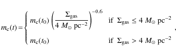
- A time-dependent IMF of the form given in Eq. (11), where
and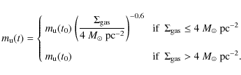
(19)
In the equations above, and
and
 denote the present-day values for the local-disc IMF.
Note that when
denote the present-day values for the local-disc IMF.
Note that when
 pc-2, this IMF is nearly identical to that of case (a).
![\begin{figure}
\par\includegraphics[width=7.5cm,clip]{13315_f3.eps}\vspace*{-2mm}
\vspace*{-2mm}
\end{figure}](/articles/aa/full_html/2010/07/aa13315-09/img76.png)
|
Figure 3: Evolution of the IMF with the gas density in model E1. Meaning of the axes as in Fig. 2. |
| Open with DEXTER | |
Table 2: Predicted and observed quantities of the solar neighbourhood.
In order to include the contribution from supernovae type Ia (SNIa)
events, which is commonly assumed to be the result of gas accretion
onto a white
dwarf from its companion (presumably a red giant) in a binary system,
the formalism introduced by Greggio & Renzini (1983) and
Matteucci & Greggio (1986) is used. In this formalism,
the equation describing the evolution of an element i can be written as
|
|
= | ||
|
|||
|
(20) | ||
|
|||
|
where
Table 3: Solar abundances by mass predicted for 4.56 years ago by the models and compared with the current solar composition derived from observations.
3 Abundance data
For the Galactic HII regions, the oxygen and carbon abundances and the distances relative to the Sun, were taken from Esteban et al. (2002; 2005). For the extragalactic HII regions, data were taken from Bergvall 1985, Garnett et al. (1995, 1997, 1999), Kobulnicky et al. (1997) and Izotov & Thuan (1999). In all cases the spectra are corrected for extinction and underlying absorption in the Balmer lines. The carbon abundances by Esteban et al. (2005) are also corrected for the presence of a carbon dust component.
Stellar abundance data were compiled from several different studies. For the solar neighbourhood, the data were compiled from several authors (Bensby & Feltzing 2006; Ecuvillon et al. 2004; Fabbian et al. 2009a; Gratton et al. 2000; Gustafsson et al. 1999, Israelian et al. 2004, Jonsell et al. 2005, Spite et al. 2005), while the Cepheid abundances in Fig. 7 were taken from the works by Andrievski et al. (2002a,b,c, 2004) and Luck et al. (2003,2006). The observed G-dwarf distributions used in this paper were taken from Edvardsson et al. (1993) and Wyse & Gilmore (1995).
Results for HI and H2 (CO) were taken from Dame (1993). To obtain a consistent and, possibly, more correct set of data for the hydrogen distributions, the conversion from CO flux to H2 surface density has been redone using the oxygen-dependent calibration by Wilson (1995), assuming the O/H-gradient derived by Esteban et al. (2002,2005).
4 Results and discussion
Using the framework described in Sect. 2 in association with a variety of nucleosynthetic prescriptions, we computed the following five types of CEMs for the Milky Way:
- (A)
- HM-star yields by WW95 and LIM-star yields by Gavilán et al. (2005)
and Gavilán et al. (2007
![[*]](/icons/foot_motif.png) ), the latter being for low-metallicity.
), the latter being for low-metallicity.
- (B)
- HM-star yields by Portinari et al. (1998) and LIM-star yields from van den Hoek & Groenewegen (1997).
- (C)
- As in model A, except that for HM-stars the carbon yields at zero metallicity (Z = 0) are increased by 50%.
- (D)
- As in model C, except that the LIM-star carbon yields below Z = 0.01 are increased by 50% in an attempt to reproduce the highest carbon abundances derived for objects having metallicities around solar.
- (E)
- Yields as in model A but now with an evolving IMF according to Eq. (18).
The model parameters were adjusted to achieve good agreement with the abundance data described in Sect. 3, i.e., either attempting to reproduce the radial trends of elemental abundances (star formation type 1, referred to as models A1-E1, see Fig. 7) or of the molecular hydrogen density as derived by (Dame 1993) from observations of the outer parts of the Galaxy (star formation type 2, referred to as models A2-D2, see Fig. 8). Other properties, such as the solar abundance pattern, the observed G-dwarf distribution and basic solar neighbourhood quantities were also used as constraints in both cases (see Tables 2, 3 and Fig. 4).
4.1 Solar neighbourhood trends
For the chemical evolution of the solar neighbourhood (defined, in the
models presented here, as the evolution at galactocentric radius
R = 8.5 kpc) prescription of type 1 and 2 for star formation
provide very similar results. Hence, only models A1-E1 will be
discussed here.
Model A1 provides satisfying results for the O/Fe trend and also a
quite good agreement with the observed C/Fe trend, except at disc-like
metallicities (
![]() ), where observations suggest a higher C/Fe (see Fig. 6). However, model A1 fails to explain the C/O trend
shown by metal-poor stars (Fig. 9). Model B1, in which a considerably larger fraction (compared to model A1, see Fig. 5)
of carbon
comes from HM-stars seems to slightly over-produce carbon relative to
iron, compared to corresponding ratios derived from observations
for the solar neighbourhood and, just as model A1, it cannot reproduce
the C/O trend at low metallicity.
), where observations suggest a higher C/Fe (see Fig. 6). However, model A1 fails to explain the C/O trend
shown by metal-poor stars (Fig. 9). Model B1, in which a considerably larger fraction (compared to model A1, see Fig. 5)
of carbon
comes from HM-stars seems to slightly over-produce carbon relative to
iron, compared to corresponding ratios derived from observations
for the solar neighbourhood and, just as model A1, it cannot reproduce
the C/O trend at low metallicity.
![\begin{figure}
\par\includegraphics[width=8.5cm,clip]{13315_f4.eps}\vspace*{-3mm}
\end{figure}](/articles/aa/full_html/2010/07/aa13315-09/img113.png)
|
Figure 4:
Predicted metallicity distribution for the solar neighbourhood G-dwarfs according to models A1-E1 convolved with a gaussian with
|
| Open with DEXTER | |
In models C1 and D1, the carbon production at zero metallicity is significantly increased, which may provide a solution to the carbon-enrichment problem at low metallicities, as suggested by Akerman et al. (2004) and Carigi et al. (2005). The Z=0 yields for HM-stars by Chieffi & Limongi (2004), provide a C/O-ratio that is consistent with that derived from observations at very low metallicity, but it is roughly the same also at moderately low metallicities where observations instead suggest that C/O becomes much lower. If the carbon yields were indeed higher than according to WW95, but only at Z = 0, it would pose an interesting problem for nucleosynthesis modelling: why do massive, essentially metal-free, stars produce much more carbon than more metal-rich ones of similarly high mass?
In the present paper, effects of inhomogeneities and contributions from pair-instability supernovae during the earliest evolution of the Galaxy are not studied, although the latter may still play an important role also for the C/O-ratio (cf. Karlsson & Gustafsson (2005, Karlsson et al. 2008). The total carbon yield may thus be significantly higher at early times, as in models C1 and D1. Despite the high carbon yields at Z=0, also models C1 and D1 are reasonably consistent with the observed C/Fe vs. Fe/H-trend at low metallicity (again, see Fig. 6). Model D1, however, is the only model that seems to explain the highest C/Fe-ratios found at the high metallicity end.
![\begin{figure}
\par\includegraphics[width=8.6cm,clip]{13315_f5.eps}\vspace*{-3mm}
\end{figure}](/articles/aa/full_html/2010/07/aa13315-09/img114.png)
|
Figure 5: Cumulative fraction of carbon due to LIM-stars as a function of time at the solar vicinity, according to model A1-E1 in this paper. |
| Open with DEXTER | |
The solar abundance pattern (taken to be the composition of the ISM at ![]() ,
4.56 Gyr ago) is well reproduced by all models - except for
an over-production of nitrogen in general and for models D1 and D2,
where the carbon abundance is about 30% too high (see Table 3)
- but it should be noted that all model parameters are calibrated such
that solar abundances and the peak of the G-dwarf distribution
(Fig. 4)
are reproduced. For disc-like metallicities, the apparent over-production of nitrogen by the models seen in Fig. 6
may be a result of
the LIM-star yields chosen for this study in combination with the
prescription for star formation. Both van den Hoek & Groenewegen (1997) and
Gavilán et al. (2005)
predict high nitrogen yields. In the low-metallicity end, however, the
models seem to underproduce nitrogen, although the
high nitrogen abundances derived from observations of some halo stars
are probably the exception rather than the rule (Israelian et al. 2004).
,
4.56 Gyr ago) is well reproduced by all models - except for
an over-production of nitrogen in general and for models D1 and D2,
where the carbon abundance is about 30% too high (see Table 3)
- but it should be noted that all model parameters are calibrated such
that solar abundances and the peak of the G-dwarf distribution
(Fig. 4)
are reproduced. For disc-like metallicities, the apparent over-production of nitrogen by the models seen in Fig. 6
may be a result of
the LIM-star yields chosen for this study in combination with the
prescription for star formation. Both van den Hoek & Groenewegen (1997) and
Gavilán et al. (2005)
predict high nitrogen yields. In the low-metallicity end, however, the
models seem to underproduce nitrogen, although the
high nitrogen abundances derived from observations of some halo stars
are probably the exception rather than the rule (Israelian et al. 2004).
![\begin{figure}
\par\includegraphics[width=9cm,clip]{13315_f6.eps} %
\end{figure}](/articles/aa/full_html/2010/07/aa13315-09/img116.png)
|
Figure 6:
Stellar abundances of carbon, nitrogen and oxygen, relative to iron in
the solar neighbourhood. All lines (models) and symbols (observations)
are explained in the figure. Data from Fabbian et al. 2009a is that derived accounting for H-collisions.
The thin dashed lines marks the solar values. Models with the second type of star formation law (A2-D2) are not shown,
but yield very similar results. The discontinuity in the model tracks seen in the carbon abundance plot around
|
| Open with DEXTER | |
Model E1, in which an evolving IMF was used, provides an alternative
solution to the early carbon-enrichment problem. Using the yields by
WW95,
without modifications, it reproduces the C/O vs. O/H trend and
simultaneously the C/Fe vs. Fe/H at low metallicity fairly well.
The reason why an evolving IMF can solve C/O vs. O/H problem using the
yields by WW95, is that the C/O-ratio of the
ejecta is much higher for stellar masses around
![]() than for more massive stars. Hence, if the IMF is peaking at
intermediate stellar masses rather than at subsolar masses, the IMF
weighted C/O-ratio is roughly 0.5 dex higher than it would be
otherwise.
Whether an evolving IMF is more likely than a scenario with high carbon
yields at Z=0
is matter of debate, but several recent
studies suggest that in the early Universe, star formation took place
according to an IMF that was more top-heavy than at present time
(see, e.g., Tumlinson 2006; Davé 2008, van Dokkum 2008,
and references therein).
than for more massive stars. Hence, if the IMF is peaking at
intermediate stellar masses rather than at subsolar masses, the IMF
weighted C/O-ratio is roughly 0.5 dex higher than it would be
otherwise.
Whether an evolving IMF is more likely than a scenario with high carbon
yields at Z=0
is matter of debate, but several recent
studies suggest that in the early Universe, star formation took place
according to an IMF that was more top-heavy than at present time
(see, e.g., Tumlinson 2006; Davé 2008, van Dokkum 2008,
and references therein).
4.2 Abundance gradients
The Fe/H-gradients predicted by the models all agree quite well with the observed Fe/H-gradient obtained from Cepheids (see Fig. 7). A similar radial trend was also found by Nordström et al. (2004) for young stars at galactocentric distances between 6 and 10 kpc.
![\begin{figure}
\par\includegraphics[width=15cm,clip]{13315_f7.eps} \vspace*{3mm}
\end{figure}](/articles/aa/full_html/2010/07/aa13315-09/img118.png)
|
Figure 7: Predicted and observed radial trends for O/H, C/H (upper panels), Fe/H and the surface density of hydrogen (lower panels) in the Milky Way for models computed using the star formation prescription of type 1. Solid circles show abundances in HII regions, while empty circles show abundances in Cepheids. The vertical and horizontal thin, dashed lines indicate the solar values according to Asplund et al. (2005). |
| Open with DEXTER | |
The results regarding the C/H-gradient are inconclusive. The ISM abundances (Esteban et al. 2005, Carigi et al. 2005) are quite high and in reasonable agreement with all models, although models C1 and C2 fit these data better (see Figs. 7 and 8). On the other hand, the Cepheid carbon abundances are significantly lower, which better matches, at solar galactocentric distance, the current solar abundance of carbon. However, the ranges of abundances seen in in the solar neighbourhood are rather wide and the Sun may therefore not represent the typical composition of the ISM in the solar neighbourhood at the time of formation of the Sun. This suggests that calibrating the parameters of the CEMs against the current solar abundance pattern may cause the present-day C/H predicted by these models to end up above (or below) that measured in young stars, which one may assume reflects the C/H of the ISM. It might be that the solar abundance pattern should not at all be used as a constraint on CEMs for the epoch when the Sun was formed, since its chemical composition (relative to iron) may depart from those of most solar-type stars of similar ages and orbits (for further discussion, see Gustafsson 2008 and references therein), in fact even from those of solar twins (Meléndez et al. 2009a,b; Nordlund 2009). In any case, the abundance difference between Cepheids and HII-regions still lacks a proper explanation.
![\begin{figure}
\par\includegraphics[width=15cm,clip]{13315_f8.eps} %
\end{figure}](/articles/aa/full_html/2010/07/aa13315-09/img119.png)
|
Figure 8: Same as Fig. 7, but for models computed using the star formation prescription of type 2. |
| Open with DEXTER | |
Models A2-D2 were designed to fit the hydrogen distribution (according to the results of Dame 1993) as well as possible. The good agreement is mainly a result of the assumption that there exists a true star-formation threshold in the disc, below which star formation will essentially cease completely in principle identical to the assumption made by, e.g., Chiappini et al. 1997 , Chiappini et al. 2001). However, the fit to the hydrogen distribution is obtained at the expense of a good fit to the abundance gradients derived from observations in the outer parts of the Galaxy. As shown in Fig. 8, the threshold causes the abundance gradients predicted by the models to fall-off steeply at galactocentric distances beyond 13 kpc, which is the part of the disc where the gas density in the model never reaches the threshold value. On the basis of this disagreement with C, O and Fe abundance gradients derived from observations, it is therefore not likely that star formation will actually cease completely when the gas density drops below the critical density.
The somewhat poorer agreement between models A1-E1 and the observed hydrogen distribution should not be seen as a major problem. In the present study, the possibility of having a slow radial gas flow has not been studied. Such a flow has not been observed, but even a very slow radial gas flow can alter the hydrogen distribution quite significantly, provided enough time is available for the process. Hence, the hypothesis presented here via models A1-E1 (i.e., that there are two modes of star formation rather than an actual threshold) is not excluded by the slight inconsistency with the HI observations of the outer disc.
![\begin{figure}
\par\includegraphics[width=12cm,clip]{13315_f9.eps}\vspace*{3mm}
\end{figure}](/articles/aa/full_html/2010/07/aa13315-09/img121.png)
|
Figure 9: Carbon abundance relative
to oxygen. Note that Galactic and extragalactic HII-regions
appear to follow a trend similar to that of the solar neighbourhood.
The different lines have the same meaning as in Figs. 4-8, i.e.,
they correspond to models A1-E1.
The yellow-shaded (bright) area indicates roughly where C stars
dominate the carbon enrichment of the ISM according to models A1, C1
and E1.
Thin squares show
data from Fabbian et al. (2009a)
assuming no hydrogen collisions in their abundance derivations, while
thick squares show the same data set,
but accounting for hydrogen collisions. The quantitative model results
are uncertain during the first few time steps, which is the reason the
plot is cut at
|
| Open with DEXTER | |
4.3 The inverse chemical evolution problem
The model of galaxy evolution described in Sect. 2 has many essentially free parameters. Nonetheless, models of this type have proven successful in several ways, e.g., by being able to simultaneously reproduce observational constraints such as the G-dwarf distribution, basic abundance patterns and the age-metallicity relation for stars in the solar neighbourhood, although the latter must be regarded as a rather uncertain constraint (see Feltzing et al. 2001). However, due to the many parameters, it is not obvious that one may take abundances derived from observations and, via CEMs, derive what stellar sources (types of stars) contribute the carbon and how the production of carbon in these stars may vary with metallicity. In principle, one has a really non-trivial inverse problem to solve, i.e., finding the stellar yields from observed abundance patterns. Basic requirements for such an attempt are that a radically different star formation history should not alter the evolution of abundance ratios too much and that the IMF is universal and non-evolving or that it is possible to specify how the IMF is evolving.
The modified sets of yields (C and D) were designed to improve the agreement between models and observations at different metallicities. However, for stellar abundances in the solar neighbourhood, low metallicity often means that the star belongs to the halo/thick disc population. The halo/thick disc population has, of course, a different formation history and therefore the evolution of elemental ratios may be slightly different. Several, very different, infall-time-scales and star formation prescriptions were tested, but such variations of the CEM did not change the predicted solar neighbourhood abundance pattern much. The two different prescriptions for star formation used in this paper (type 1 and 2) provide very similar abundance trends for the solar neighbourhood with only minimal changes to other model parameters. In fact, the IMF and the stellar yields, or the IMF-weighted integrated yields, turn out to be the most critical ingredients. Changes in the integrated yields will dominate over reasonable variations of all other parameters. It is therefore possible to use CEMs to analyse how stellar yields may vary with stellar mass and metallicity to be consistent with observations, provided that the IMF (and its possible evolution) is known.
It seems that the carbon abundances in stars at low metallicity in the solar neighbourhood cannot be explained by a standard Galactic evolution scenario and commonly used stellar yields (cf. model A1 and B1). Consequently, modifying the yields to obtain better agreement with observations, as a solution to the inverse chemical evolution problem, may therefore be a justified measure. However, as model E1 shows, abandoning the idea of a universal and non-evolving IMF, may just as well be the solution to the carbon-enrichment problem for the early stages of Galactic evolution. Observed abundances (except those of extremely metal-poor stars, perhaps) reflect the enrichment from a stellar population, and therefore one must be careful suggesting that abundances derived from observations pose a challenge to nucleosynthesis models and stellar evolution theory. We are left with two main options: (a) the carbon yields of essentially metal-free HM-stars must be much higher than predicted by WW95, or (b) the IMF evolves with time and/or is not completely universal. A necessary prerequisite for actually solving the carbon enrichment problem is thus to establish which hypothesis holds. In case both (a) and (b) is true, this would require a much less top-heavy IMF at early times, which may not be consistent with observational constraints of some extremely metal-poor halo stars.
The carbon enrichment at later stages (thin disc evolution) can
also be explained in two ways, either: (a) the carbon contribution from
HM-stars
is metallicity-dependent in such a way that it increases significantly
with metallicity during the thin disc evolution, or (b) the rising
trend
is due to a significant contribution from the long-lived stars (with
masses
![]() )
that becomes important only after a few Gyr. Scenario
(a) is the one advocated by Gustafsson et al. (1999), while (b) represents the picture favoured by several authors
(e.g., Chiappini et al. 2003; Akerman et al. 2004; Gavilán et al. 2005), in
which up to 80% of the carbon in the present-day ISM may be due to LIM-stars (see Fig. 5). It is virtually impossible to distinguish
between (a) and (b) just by considering abundance data, but the fact that carbon and iron seem to be released to the ISM on similar
time-scales, suggests that these two elements originate from stars that evolve
on similar time-scales. If LIM-stars produce most of the carbon and
supernovae Type Ia produce the bulk of iron in the Galaxy, the rather
flat trend of C/Fe with Fe/H would be explained naturally
(Bensby & Feltzing 2006).
If, instead, scenario (a) is correct, it would require that the
metallicity dependence of the carbon yields of HM-stars is fine-tuned
with the SNIa-produced Fe in such a way that both the flat C/Fe vs.
Fe/H trend and the rising C/O vs. O/H trend are reproduced.
Thus, while (a) is a plausible hypothesis, scenario (b) is simpler in
that it does not require that the yields have any specific metallicity
dependence; it only requires that LIM-stars produce most of the carbon,
so that the carbon enrichment of the ISM is delayed.
)
that becomes important only after a few Gyr. Scenario
(a) is the one advocated by Gustafsson et al. (1999), while (b) represents the picture favoured by several authors
(e.g., Chiappini et al. 2003; Akerman et al. 2004; Gavilán et al. 2005), in
which up to 80% of the carbon in the present-day ISM may be due to LIM-stars (see Fig. 5). It is virtually impossible to distinguish
between (a) and (b) just by considering abundance data, but the fact that carbon and iron seem to be released to the ISM on similar
time-scales, suggests that these two elements originate from stars that evolve
on similar time-scales. If LIM-stars produce most of the carbon and
supernovae Type Ia produce the bulk of iron in the Galaxy, the rather
flat trend of C/Fe with Fe/H would be explained naturally
(Bensby & Feltzing 2006).
If, instead, scenario (a) is correct, it would require that the
metallicity dependence of the carbon yields of HM-stars is fine-tuned
with the SNIa-produced Fe in such a way that both the flat C/Fe vs.
Fe/H trend and the rising C/O vs. O/H trend are reproduced.
Thus, while (a) is a plausible hypothesis, scenario (b) is simpler in
that it does not require that the yields have any specific metallicity
dependence; it only requires that LIM-stars produce most of the carbon,
so that the carbon enrichment of the ISM is delayed.
An interesting fact, which deserves further study (beyond the scope of this paper), is evident from data plotted in Fig. 9. Extragalactic HII-regions show C/O-ratios which line up along the same trend with O/H as the stars in the solar neighbourhood: metal-poor (low-mass) galaxies show low carbon abundances, while more metal-rich galaxies show considerably higher carbon abundances, relative to oxygen. This may, in principle, be consistent with both scenario (a) and (b) just discussed for the thin disc. Carbon production in the Galactic disc appears to be coupled with the age/metallicity of the stellar population. Similarly, it seems that the carbon abundance in extragalactic HII-regions is coupled with the age of the dominant stellar population or the overall metallicity. However, if (b) is the correct scenario, metal-poor galaxies must be dominated by young stellar populations, so that the majority of LIM-stars have not yet evolved off the main sequence, thus locking carbon, without significantly enriching the ISM. Nevertheless, the light distribution of HII/BCG galaxies reveals the presence of a significant low surface-brightness population of old stars (Telles et al. 1997; Kunth & Östlin 2000), although it is difficult to determine the mass fraction of such an underlying population. If scenario (b) can be confirmed, metal-poor galaxies are very likely to have formed most of their stars quite recently, since a significant old population would raise the C/O-ratio due to enrichment from LIM-stars.
It is often suggested (see Kunth & Östlin 2000, and references therein) that low-mass, metal-poor galaxies are deficient in metals due to significant galactic winds and may therefore have undergone several star-forming episodes in the past. Galactic winds may be responsible for maintaining low over-all metallicities, but cannot easily explain low C/O-ratios unless the winds are extremely selective (oxygen remains while carbon is expelled from the galaxy) in scenario (b). The fundamental question is then whether LIM-stars are (or not) the main contributors to carbon nucleosynthesis in metal-poor galaxies, and if galactic winds may maintain low over-all metallicities even after a sequence of star-forming episodes.
4.4 Uncertainties in iron production
Several uncertainties have not been addressed in detail here. One, particularly important, is the production of iron, which cannot be well-constrained for two reasons: the location of the mass cut (that divides the part of the star that collapses in the remnant from that which is expelled) in supernova nucleosynthesis models is a free (although restricted) parameter, and the origin of supernovae Type Ia (SNIa) is not fully understood.
The iron yields by WW95 show a dependence on metallicity (possibly an effect of how the mass
cut was chosen), which may not be realistic. At Z=0 the IMF-weighted WW95 yields show an O/Fe-ratio that is much lower than the ratios
derived from observations in very metal-poor stars ([O/Fe] ![]() when
when
![]() ,
see Fig. 6), which is the reason why the iron
yields at Z
= 0 have been lowered to 1/5 of their original values in the models
presented in this paper. However, non-local thermal equilibrium
(non-LTE) effects on oxygen lines may explain the O/Fe discrepancy.
Including corrections for non-LTE effects, smaller
[O/Fe] values are derived from observations, so the [O/Fe] may actually
agree quite well with WW95 (Fabbian et al. 2006; Fabbian et al. 2009b).
,
see Fig. 6), which is the reason why the iron
yields at Z
= 0 have been lowered to 1/5 of their original values in the models
presented in this paper. However, non-local thermal equilibrium
(non-LTE) effects on oxygen lines may explain the O/Fe discrepancy.
Including corrections for non-LTE effects, smaller
[O/Fe] values are derived from observations, so the [O/Fe] may actually
agree quite well with WW95 (Fabbian et al. 2006; Fabbian et al. 2009b).
The fact that the iron yields of HM-stars are rather uncertain, and models of the evolution of SNIa rates cannot be very well constrained from observations, makes the common practice of using iron as the reference element (representing the over-all metallicity) somewhat questionable when comparing data and models. Hence, it makes more sense to calibrate CEMs primarily against abundances relative to, e.g., oxygen or other common elements for which the enrichment essentially follows the star formation rate. Therefore, focus is on reproducing C/H, O/H and C/O, rather than C/Fe and O/Fe, in the present study.
4.5 Uncertainties in carbon production: effects of carbon star mass loss
There are many assumptions and physical prescriptions that may affect the nucleosynthesis in stellar evolution models. For LIM-stars the duration of the AGB phase and the number of thermal pulses is almost uniquely determined by the mass-loss rate. The evolution of the internal structure depends on the mass-loss rate as well (Blöcker 1995), which in turn affects the fundamental stellar parameters. Since the mass-loss rate depends on these stellar parameters, there will be a feedback, which means that the mass-loss prescription put into a stellar evolution model is critical, and it is indeed well-known that changing the mass-loss prescription can have profound effects on the yields of AGB stars (see, e.g., van den Hoek & Groenewegen 1997). More precisely, the sum of carbon and nitrogen synthesised in LIM stars is largely controlled by the mass-loss rate on the AGB.
In the work of Gavilán et al. (2005) it was assumed that stars of low metallicity have smaller total radii (yielding higher surface gravity) and thus less effective mass-loss, which increases the lifetime of the AGB phase and allows these stars to experience several more dredge-up events where carbon is mixed into the envelope. At late stages, as metallicity increases, the carbon production declines, and secondary nitrogen production becomes increasingly significant (see also Buell 1997, for further details). But is it correct to assume that low metallicity means less effective mass-loss relative to that of solar metallicity stars?
Mattsson et al. (2008)
have shown that, according to theoretical models, the overall
metallicity is not affecting dust-driven mass-loss from C-stars much at
all. It is mainly the abundance of carbon, available for dust
formation, that has a significant effect.
The dust-driven mass-loss takes place mainly during the late stages of
evolution, where thermal pulses and dredge-up events dominate the
evolution. There is no particular reason to assume that low metallicity
C-stars will experience more thermal pulses and dredge-up events before
the
termination of the AGB. Furthermore, Mattsson et al. (in prep.)
present a state-of-the-art model of the late stages of evolution of a ![]() -star
using a new detailed mass-loss prescription based on the results by Mattsson et al. (2010)
and a new set of low-temperature opacity coefficients,
in which effects of the abundances of carbon and oxygen were taken into
account. This resulted in a significantly lower effective temperature
and
the development of a very pronounced so-called superwind, shortly after
the star had become carbon rich, which terminated the C-star evolution
after only few thermal pulses. The amount of carbon that can be dredged
up and expelled by the stellar wind is therefore limited. No final word
yet, but these recent findings seem to restrict the carbon production
in LIM-stars by means of a self-regulating process, where the mass-loss
rate increases with every dredge-up event associated with each thermal
pulse.
-star
using a new detailed mass-loss prescription based on the results by Mattsson et al. (2010)
and a new set of low-temperature opacity coefficients,
in which effects of the abundances of carbon and oxygen were taken into
account. This resulted in a significantly lower effective temperature
and
the development of a very pronounced so-called superwind, shortly after
the star had become carbon rich, which terminated the C-star evolution
after only few thermal pulses. The amount of carbon that can be dredged
up and expelled by the stellar wind is therefore limited. No final word
yet, but these recent findings seem to restrict the carbon production
in LIM-stars by means of a self-regulating process, where the mass-loss
rate increases with every dredge-up event associated with each thermal
pulse.
5 Conclusions and final remarks
CEMs for the Milky Way have been presented. Four different nucleosynthesis prescriptions were used, where two contain ad hoc modifications to meet the abundance trends of C/O vs. O/H and C/Fe vs. Fe/H derived from observations. According to these CEMs one may conclude the following:
- Carbon is being released to the ISM on time-scales comparable to that of iron, which is produced mainly by supernovae Type Ia.
- An evolving IMF, being top-heavy (favouring the formation of HM-stars) during the early stages of Galactic evolution, can explain the C/O vs. O/H trend seen in the abundances derived by Fabbian et al. (2009a), without violating any other observational constraints.
- The C/H-gradient (or the metallicity gradient in general)
derived from observations in the Milky Way disc suggest there is a
problem with simple CEMs and the hydrogen distribution. Introducing a
star formation threshold at
 pc-2
can explain the shape of the hydrogen distribution, but such a model
predicts a steep fall-off in all abundance gradients beyond a certain
galactocentric distance and cannot explain the flattening of the C/H
and Fe/H gradients of the outer disc traced by Cepheid observations. It
is possible that radial gas flows in the outer disc in combination with
a ``low-efficiency mode'' of star formation is responsible for the
abundance gradients and the hydrogen distribution.
pc-2
can explain the shape of the hydrogen distribution, but such a model
predicts a steep fall-off in all abundance gradients beyond a certain
galactocentric distance and cannot explain the flattening of the C/H
and Fe/H gradients of the outer disc traced by Cepheid observations. It
is possible that radial gas flows in the outer disc in combination with
a ``low-efficiency mode'' of star formation is responsible for the
abundance gradients and the hydrogen distribution.
- HM-star yields of carbon and oxygen probably have a metallicity dependence, as argued by Gustafsson et al. (1999), but the observed increase with metallicity of the C/O-ratio seen in disc stars could just as well be due to a delayed release of carbon from LIM-stars. If the best-fit models are correct, the major source of carbon in the present-day Galaxy is the LIM-stars, providing as much as 80% of the carbon to the ISM. Although HM-stars as major carbon producers cannot be excluded, the LIM-star scenario provides a simpler explanation, which does not require that carbon yields depend strongly on metallicity.
That LIM-stars may contribute most of the carbon in the solar neighbourhood has previously been concluded by several other authors (e.g., Chiappini et al. 2003; Akerman et al. 2004; Gavilán et al. 2005). The C/Fe vs. Fe/H trend seen in unevolved, metal-poor stars in the solar neighbourhood suggests that the contribution from HM-stars at low metallicity must be limited, unless these stars also have an enhanced iron production, and the contribution has to increase dramatically with metallicity to explain the sharp up-turn in C/O vs. O/H, seen in Fig. 9. If HM-stars were the main contributors, then the carbon yields of these stars (around and above solar metallicity) must be even larger than the oxygen yields. Maeder (1992) and Portinari et al. (1998) have computed models where such results were obtained, and more recent work seems to give similar results (see, e.g., Meynet & Maeder 2002, 2003, 2005). But models of HM-star evolution are also riddled by several uncertainties.
Finally, returning to the connection between the cosmic carbon
abundance and carbon-based life, one may notice that in the outer parts
of the Milky Way disc, where the peak of star formation was reached
quite recently (or has not yet been reached), there has not been enough
time for the bulk of LIM-stars (especially those with main-sequence
masses below
![]() )
to evolve into mass-losing C-stars, or the metallicity is not large
enough if the HM-star carbon production scenario is instead the correct
one.
Are the outer parts of the Galaxy therefore excluded as a possible
environment for complex life to emerge, since there has been no
significant carbon enrichment until quite recently?
)
to evolve into mass-losing C-stars, or the metallicity is not large
enough if the HM-star carbon production scenario is instead the correct
one.
Are the outer parts of the Galaxy therefore excluded as a possible
environment for complex life to emerge, since there has been no
significant carbon enrichment until quite recently?
The author wishes to thank the referee for all valuable comments and suggestions that helped improve the clarity and readability of the paper. Bengt Gustafsson, Nils Bergvall and Kjell Olofsson are thanked for their valuable comments on a draft version of this paper. Mercedes Mollá and Marta Gavilán are thanked for clarifying some issues regarding the LIM-star yields.
References
- Abel, T., Bryan, G. L., & Norman, M. L. 2002, Science, 295, 93 [NASA ADS] [CrossRef] [PubMed] [Google Scholar]
- Akerman, C. J., Carigi, L., Nissen, P. E., Pettini, M., & Asplund, M. 2004, A&A, 414, 931 [NASA ADS] [CrossRef] [EDP Sciences] [Google Scholar]
- Andrievsky, S. M., Kovtyukh, V. V., Luck, R. E., et al. 2002a, ApJ, 381, 32 [Google Scholar]
- Andrievsky, S. M., Bersier, D., Kovtyukh, V. V., et al. 2002b, ApJ, 384, 140 [Google Scholar]
- Andrievsky, S. M., Kovtyukh, V. V., Luck, R. E., et al. 2002c, ApJ, 392, 491 [Google Scholar]
- Andrievsky, S. M., Luck, R. E., Martin, P., & Lépine, J. R.D. 2004, ApJ, 413, 159 [Google Scholar]
- Asplund, M., Grevesse, N., & Sauval, A. J. 2005, ASPC, 336, 25 [Google Scholar]
- Bensby, T., & Feltzing, S. 2006, MNRAS, 367, 1181 [NASA ADS] [CrossRef] [Google Scholar]
- Bergvall, N. 1985, A&A, 146, 269 [NASA ADS] [Google Scholar]
- Blöcker, T. 1995, A&A, 297, 727 [NASA ADS] [Google Scholar]
- Boissier, S., Prantzos, N., Boselli, A., & Gavazzi, G. 2003, MNRAS, 346, 1215 [NASA ADS] [CrossRef] [Google Scholar]
- Burbidge, E. M., Burbidge, G. R., Fowler, W. A., & Hoyle F. 1957, Rev. Mod. Phys., 29, 547 [NASA ADS] [CrossRef] [Google Scholar]
- Buell, J. F. 1997, Ph.D. Thesis, Univ. of Oklahoma [Google Scholar]
- Carigi, L., Peimbert, M., Esteban, C., & García-Rojas, J. 2005, ApJ, 623, 213 [NASA ADS] [CrossRef] [Google Scholar]
- Chabrier, G. 2003, PASP, 115, 763 [Google Scholar]
- Chieffi, A., & Limongi, M. 2004, ApJ, 608, 405 [NASA ADS] [CrossRef] [Google Scholar]
- Chiosi, C. 1980, A&A, 83, 206 [NASA ADS] [Google Scholar]
- Cayrel, R., Depagne, E., Spite, M., et al. 2004, A&A, 416, 1117 [NASA ADS] [CrossRef] [EDP Sciences] [Google Scholar]
- Chiappini, C., Matteucci, F., & Gratton, R. 1997, ApJ, 477, 765 [NASA ADS] [CrossRef] [Google Scholar]
- Chiappini, C., Matteucci, F., & Padoan, P. 2000, ApJ, 528, 711 [NASA ADS] [CrossRef] [Google Scholar]
- Chiappini, C., Matteucci, F., & Romano, D. 2001, ApJ, 554, 1044 [NASA ADS] [CrossRef] [Google Scholar]
- Chiappini, C., Romano, D., & Matteucci, F. 2003, MNRAS, 339, 63 [NASA ADS] [CrossRef] [Google Scholar]
- Chiappini, C., Hirschi, R., Meynet, S., Ekström, S., Maeder, A., & Matteucci, F. 2006, A&A, 449, L27 [NASA ADS] [CrossRef] [EDP Sciences] [Google Scholar]
- Dame, T. M. 1993, in Back to the Galaxy, ed. S. Holt, & F. Verter (New York: Springer), 267 [Google Scholar]
- Davé, R. 2008, MNRAS, 385, 147 [NASA ADS] [CrossRef] [Google Scholar]
- Dearborn, D., Schramm, D. N., & Tinsley, B. M. 1978, ApJ, 223, 557 [NASA ADS] [CrossRef] [Google Scholar]
- van Dokkum, P. G. 2008, ApJ, 674, 29 [NASA ADS] [CrossRef] [Google Scholar]
- Ecuvillon, A., Israelian, G., Santos, N. C., et al. 2004, A&A, 418, 703 [NASA ADS] [CrossRef] [EDP Sciences] [Google Scholar]
- Edvardsson, B., Andersen, J., Gustafsson, B., et al. 1993, A&A, 275, 101 [NASA ADS] [Google Scholar]
- Elmegreen, B. 1999, ApJ, 515, 323 [NASA ADS] [CrossRef] [Google Scholar]
- Esteban, C., Peimbert, M., Torres-Peimbert, S., & Rodríguez, M. 2002, ApJ, 581, 241 [NASA ADS] [CrossRef] [Google Scholar]
- Esteban, C., García-Rojas, J., Peimbert, M., et al. 2005, ApJ, 618, L95 [NASA ADS] [CrossRef] [Google Scholar]
- Fabbian, D., Asplund, M., Carlsson, M., & Kiselman, D. 2006, A&A, 458, 899 [NASA ADS] [CrossRef] [EDP Sciences] [Google Scholar]
- Fabbian, D., Nissen, P. E., Asplund, M., Pettini, M., & Akerman, C. 2009a, A&A, 500, 1143 [NASA ADS] [CrossRef] [EDP Sciences] [Google Scholar]
- Fabbian, D., Asplund, M., Barklem, P. S., Carlsson, M., & Kiselman, D. 2009b, A&A, 500, 1221 [NASA ADS] [CrossRef] [EDP Sciences] [Google Scholar]
- Feltzing, S., Holmberg, J., & Hurley, J. R. 2001, A&A, 377, 911 [NASA ADS] [CrossRef] [EDP Sciences] [Google Scholar]
- Fuchs, B., Jahreiss ,H., & Flynn, C. 2009, AJ, 137, 266 [NASA ADS] [CrossRef] [Google Scholar]
- Garnett, D. R., Skillman, E. D., Dufour, R. J., et al. 1995, ApJ, 443, 64 [NASA ADS] [CrossRef] [Google Scholar]
- Garnett, D. R., Skillman, E. D., Dufour, R. J., & Shields, G. A. 1997, ApJ, 481, 174 [CrossRef] [Google Scholar]
- Gavilán, M., Buell, J. F., & Mollá, M. 2005, A&A, 432, 861 [NASA ADS] [CrossRef] [EDP Sciences] [Google Scholar]
- Gratton, R. G., Sneden, C., Carretta, E., & Bragaglia, A. 2000, A&A, 354, 169 [NASA ADS] [Google Scholar]
- Greggio, L., & Renzini, A. 1983, A&A, 118, 217 [NASA ADS] [Google Scholar]
- Gustafsson, B., Karlsson, T., Olsson, E., Edvardsson, B., & Ryde, N. 1999, A&A, 342, 426 [NASA ADS] [Google Scholar]
- Gustafsson, B. 2008, Ph. Scr., T130 [Google Scholar]
- van den Hoek, L. B., & Groenewegen, M. A. T. 1997, A&AS, 123, 305 [NASA ADS] [CrossRef] [EDP Sciences] [Google Scholar]
- Helmi, A. 2008, A&ARv, 15, 145 [NASA ADS] [Google Scholar]
- Holmberg, J., & Flynn, C. 2004, MNRAS, 352, 440 [NASA ADS] [CrossRef] [Google Scholar]
- Hubble, E. 1923, PA, 31, 644 [NASA ADS] [Google Scholar]
- Israelian, G., Ecuvillon, A., Rebolo, R., et al. 2004, A&A, 421, 649 [NASA ADS] [CrossRef] [EDP Sciences] [Google Scholar]
- Izotov, Y. I., & Thuan, T. X. 1999, ApJ, 511, 639 [NASA ADS] [CrossRef] [Google Scholar]
- Izzard, R. G., Tout, C. A., Karakas, A. I., & Pols, O. P. 2004, MNRAS, 350, 407 [NASA ADS] [CrossRef] [Google Scholar]
- Jeans, J. H. 1902, Philos. Trans. R. Soc. London, A, 199, 1 [Google Scholar]
- Jonsell, K., Edvardsson, B., Gustafsson, B., et al. 2005, A&A, 440, 321 [NASA ADS] [CrossRef] [EDP Sciences] [Google Scholar]
- Karakas, A., & Lattanzio, J. C. 2007, PASA, 24, 103 [NASA ADS] [CrossRef] [Google Scholar]
- Karlsson, T., & Gustafsson, B. 2005, A&A, 436, 879 [NASA ADS] [CrossRef] [EDP Sciences] [Google Scholar]
- Karlsson, T., Johnson, J. L., & Bromm, V. 2008, ApJ, 679, 6 [NASA ADS] [CrossRef] [Google Scholar]
- Kennicutt, R. C. 1989, ApJ, 344, 685 [NASA ADS] [CrossRef] [Google Scholar]
- Kobulnicky, H. A., Skillman, E. D. Roy, J.-R., Walsh, J., & Rosa, M. 1997, ApJ, 477, 679 [NASA ADS] [CrossRef] [Google Scholar]
- Kunth, D., & Östlin, G. 2000, A&ARv, 10, 1 [NASA ADS] [CrossRef] [Google Scholar]
- Lacey; C. G., & Fall; S. M. 1985, ApJ, 290, 154 [NASA ADS] [CrossRef] [Google Scholar]
- Larson; R. B. 1995, MNRAS, 272, 213 [NASA ADS] [Google Scholar]
- Larson; R. B. 1996, in The Interplay Between Massive Star Formation, the ISM and Galaxy Evolution, ed., D. Kunth, B. Guiderdoni, M. Heydari-Malayeri, & T. X. Thuan (Gif sur Yvette : Editions Frontieres), 3 [Google Scholar]
- Larson, R. B. 1998, MNRAS, 301, 569 [NASA ADS] [CrossRef] [Google Scholar]
- Luck, R. E., Gieren, W. P., Andrievsky, S. M, et al. 2003, A&A, 401, 939 [NASA ADS] [CrossRef] [EDP Sciences] [Google Scholar]
- Luck, R. E., Kovtyukh, V. V., & Andrievsky, S. M. 2006, AJ, 132, 902 [NASA ADS] [CrossRef] [Google Scholar]
- Maeder, A. 1992, A&A, 264, 105 [NASA ADS] [Google Scholar]
- Marigo, P. 2001, A&A, 370, 194 [NASA ADS] [CrossRef] [EDP Sciences] [Google Scholar]
- Marigo, P. 2002, A&A, 387, 507 [NASA ADS] [CrossRef] [EDP Sciences] [Google Scholar]
- Matteucci, F., & Greggio, L. 1986, A&A, 154, 279 [NASA ADS] [Google Scholar]
- Matteucci, F., & Francois, P. 1989, MNRAS, 239, 885 [NASA ADS] [CrossRef] [Google Scholar]
- Mattsson, L., Whalin, R., & Höfner, S. 2010, A&A, 509, 14 [Google Scholar]
- Mattsson, L., Whalin, R., Höfner, S., & Erkisson, K. 2008, A&A, 484, L5 [NASA ADS] [CrossRef] [EDP Sciences] [Google Scholar]
- Melndez, J., Asplund, M., Gustafsson, B., & Yong, D. 2009a, ApJ, 704, L66 [NASA ADS] [CrossRef] [Google Scholar]
- Melndez, J., Asplund, M., Gustafsson, B., Yong, D., & Ramirez, I. 2009b, Proc. IAU Symp. 265, [arXiv:0910.0875] [Google Scholar]
- Meynet, G., & Maeder, A. 2002, A&A, 390, 561 [NASA ADS] [CrossRef] [EDP Sciences] [Google Scholar]
- Meynet, G., & Maeder, A. 2003, A&A, 404, 975 [NASA ADS] [CrossRef] [EDP Sciences] [Google Scholar]
- Meynet, G., & Maeder, A. 2005, A&A, 429, 581 [Google Scholar]
- Nordlund, Å. 2009, ApJ, submitted, [arXiv:0908.3479] [Google Scholar]
- Nordström, B., Mayor, M., Andersen, J., et al. 2005, A&A, 418, 989 [Google Scholar]
- Ohja, D. K. 2001, MNRAS, 322, 426 [NASA ADS] [CrossRef] [Google Scholar]
- Porcel, C., Garzón, F., Jiminéz-Vicente, J., & Battaner, E. 1998, A&A, 330, 136 [NASA ADS] [Google Scholar]
- Portinari, L., Chiosi, C., & Bressan, A. 1998, A&A, 334, 505 [NASA ADS] [Google Scholar]
- Preston, G. W., Shectman, S. A., & Beers, T. C. 1991, ApJ, 375, 121 [NASA ADS] [CrossRef] [Google Scholar]
- Renda, A., Kawata, D., Fenner, Y., & Gibson, B. K. 2005, MNRAS, 356, 1070 [Google Scholar]
- Renzini, A., & Voli, M. 1981, A&A, 94, 175 [NASA ADS] [Google Scholar]
- Ruphy, S., Robin, A. C., Epchtein, N., et al. 1996, A&A, 313, L21 [NASA ADS] [Google Scholar]
- Salpeter, E. E. 1952, ApJ, 115, 326 [Google Scholar]
- Salpeter, E. E. 1955, ApJ, 121, 161 [Google Scholar]
- Scalo, J. 1986, Fund. Cosm. Phys., 11, 1 [Google Scholar]
- Schaller, G., Schaerer, D., Maeder, A., & Meynet, G. 1992, A&AS, 96, 269 [Google Scholar]
- Sofue, Y., Tutui, Y., Honma, M., et al. 1999, ApJ, 523, 136 [NASA ADS] [CrossRef] [Google Scholar]
- Spite, M., Cayrel, R., Plez, B., et al. 2005, A&A, 430, 655 [NASA ADS] [CrossRef] [EDP Sciences] [Google Scholar]
- Talbot, R. J., & Arnett, D. W. 1971, ApJ, 170, 409 [NASA ADS] [CrossRef] [Google Scholar]
- Talbot, R. J., & Arnett, D. W. 1973, ApJ, 186, 51 [NASA ADS] [CrossRef] [Google Scholar]
- Telles, E., Melnick, J., & Terlevich, R. 1997, MNRAS, 288, 78 [NASA ADS] [CrossRef] [Google Scholar]
- Timmes, F. X., Woosley, S. E., & Weaver, T. A. 1995, ApJ, 98, 617 [Google Scholar]
- Tumlinson, J. 2006, ApJ, 641, 1 [NASA ADS] [CrossRef] [Google Scholar]
- Wilson, C. D. 1995, ApJ, 448, L97 [NASA ADS] [CrossRef] [Google Scholar]
- Woosley, S. E., & Weaver, T. A. 1995, ApJS, 110, 277 [Google Scholar]
- Wyse, R. F. G., & Gilmore, G. 1995, ApJ, 339, 700 [Google Scholar]
- Wyse, R. F. G., & Silk, J. 1989, ApJ, 339, 700 [NASA ADS] [CrossRef] [Google Scholar]
Footnotes
All Tables
Table 1: Parameters for the CEMs.
Table 2: Predicted and observed quantities of the solar neighbourhood.
Table 3: Solar abundances by mass predicted for 4.56 years ago by the models and compared with the current solar composition derived from observations.
All Figures
|
|
Figure 1: The Gaussian surface density profile adopted for the halo/thick disc in this paper compared to a Hubble (1923) profile, normalised to the density at the Sun's galactocentric distance (marked by a vertical dashed line in the figure). |
| Open with DEXTER | |
| In the text | |
|
|
Figure 2:
Comparison between the IMF |
| Open with DEXTER | |
| In the text | |
|
|
Figure 3: Evolution of the IMF with the gas density in model E1. Meaning of the axes as in Fig. 2. |
| Open with DEXTER | |
| In the text | |
|
|
Figure 4:
Predicted metallicity distribution for the solar neighbourhood G-dwarfs according to models A1-E1 convolved with a gaussian with
|
| Open with DEXTER | |
| In the text | |
|
|
Figure 5: Cumulative fraction of carbon due to LIM-stars as a function of time at the solar vicinity, according to model A1-E1 in this paper. |
| Open with DEXTER | |
| In the text | |
|
|
Figure 6:
Stellar abundances of carbon, nitrogen and oxygen, relative to iron in
the solar neighbourhood. All lines (models) and symbols (observations)
are explained in the figure. Data from Fabbian et al. 2009a is that derived accounting for H-collisions.
The thin dashed lines marks the solar values. Models with the second type of star formation law (A2-D2) are not shown,
but yield very similar results. The discontinuity in the model tracks seen in the carbon abundance plot around
|
| Open with DEXTER | |
| In the text | |
|
|
Figure 7: Predicted and observed radial trends for O/H, C/H (upper panels), Fe/H and the surface density of hydrogen (lower panels) in the Milky Way for models computed using the star formation prescription of type 1. Solid circles show abundances in HII regions, while empty circles show abundances in Cepheids. The vertical and horizontal thin, dashed lines indicate the solar values according to Asplund et al. (2005). |
| Open with DEXTER | |
| In the text | |
|
|
Figure 8: Same as Fig. 7, but for models computed using the star formation prescription of type 2. |
| Open with DEXTER | |
| In the text | |
|
|
Figure 9: Carbon abundance relative
to oxygen. Note that Galactic and extragalactic HII-regions
appear to follow a trend similar to that of the solar neighbourhood.
The different lines have the same meaning as in Figs. 4-8, i.e.,
they correspond to models A1-E1.
The yellow-shaded (bright) area indicates roughly where C stars
dominate the carbon enrichment of the ISM according to models A1, C1
and E1.
Thin squares show
data from Fabbian et al. (2009a)
assuming no hydrogen collisions in their abundance derivations, while
thick squares show the same data set,
but accounting for hydrogen collisions. The quantitative model results
are uncertain during the first few time steps, which is the reason the
plot is cut at
|
| Open with DEXTER | |
| In the text | |
Copyright ESO 2010
Current usage metrics show cumulative count of Article Views (full-text article views including HTML views, PDF and ePub downloads, according to the available data) and Abstracts Views on Vision4Press platform.
Data correspond to usage on the plateform after 2015. The current usage metrics is available 48-96 hours after online publication and is updated daily on week days.
Initial download of the metrics may take a while.