| Issue |
A&A
Volume 515, June 2010
|
|
|---|---|---|
| Article Number | A3 | |
| Number of page(s) | 12 | |
| Section | Extragalactic astronomy | |
| DOI | https://doi.org/10.1051/0004-6361/200913188 | |
| Published online | 28 May 2010 | |
Evolution of blue E/S0 galaxies from z
 1: merger remnants or disk-rebuilding galaxies?
M. Huertas-Company1,2,3 - J. A. L. Aguerri4 - L. Tresse5 - M. Bolzonella6 - A. M. Koekemoer7 - C. Maier8
1 - ESO, Alonso de Cordova 3107, Casilla 19001, Vitacura, Santiago,
Chile
2 - GEPI - Observatoire de Paris, Section de Meudon, 5 Place Jules
Janssen, 92190 - Meudon, France
3 - University of Paris Denis Diderot, 75205 Paris Cedex 13, France
4 - Instituto de Astrofísica de Canarias, C/ vía Láctea s/n, 38200 La
Laguna, Spain
5 - LAM-CNRS Université de Provence, 38 rue Frédéric Joliot-Curie,
13388 Marseille Cedex 13, France
6 - INAF - OA Bologna, via Ranzani 1, 40127 Bologna, Italy
7 - Space Telescope Science Institute 3700 San Martin Drive, Baltimore
MD 21218, USA
8 - Institute of Astronomy, Swiss Federal Institute of Technology (ETH
Hönggerberg), 8093 Zürich, Switzerland
Received 26 August 2009 / Accepted 4 February 2010
Abstract
Context. Studying outliers from the bimodal
distribution of galaxies in the color-mass space, such as morphological
early-type galaxies residing in the blue cloud (blue E/S0s),
can help for better understanding the physical mechanisms that lead
galaxy migrations in this space.
Aims. In this paper we try to bring new clues to
studying the evolution of the properties of a significant sample of
blue E/S0 galaxies in the COSMOS field.
Methods. We define blue E/S0 galaxies as objects
having a clear early-type morphology on the HST/ACS images
(according to our automated classification scheme GALSVM)
but with a blue rest-frame color (defined by using the SED best-fit
template on the COSMOS primary photometric catalogs). Combining these
two measurements with spectroscopic redshifts from the
zCOSMOS 10k release, we isolated 210
![]() blue early-type galaxies with
blue early-type galaxies with ![]() in three redshift bins (
0.2<z<0.55,
0.55<z<0.8,
0.8<z<1.4) and studied the evolution
of their properties (number density, SFR, morphology, size).
in three redshift bins (
0.2<z<0.55,
0.55<z<0.8,
0.8<z<1.4) and studied the evolution
of their properties (number density, SFR, morphology, size).
Results. The threshold mass (![]() ), defined at z=0
in previous studies as the mass below which the population of blue
early-type galaxies starts to be abundant relative to
passive E/S0s, evolves from
), defined at z=0
in previous studies as the mass below which the population of blue
early-type galaxies starts to be abundant relative to
passive E/S0s, evolves from ![]()
![]() 0.35 at
0.35 at ![]() to
to ![]()
![]() 0.35 at
0.35 at ![]() .
Interestingly, it follows the evolution of the crossover mass between
the early and late type populations (bimodality mass) indicating that
the abundance of blue E/S0 is another measure of the
downsizing effect in the build-up of the red sequence. There seems to
be a turn-over mass in the nature of
blue E/S0 galaxies. Above
.
Interestingly, it follows the evolution of the crossover mass between
the early and late type populations (bimodality mass) indicating that
the abundance of blue E/S0 is another measure of the
downsizing effect in the build-up of the red sequence. There seems to
be a turn-over mass in the nature of
blue E/S0 galaxies. Above ![]() blue E/S0 resemble to merger remnants probably migrating to
the red sequence on a time scale of
blue E/S0 resemble to merger remnants probably migrating to
the red sequence on a time scale of ![]() Gyr. Below this
mass, they seem to be closer to normal late-type galaxies,
as if they were the result of minor mergers that triggered the
central star formation and built a central bulge component or were
(re)building a disk from the surrounding gas in a much longer time
scale, suggesting that they are moving back or staying in the blue
cloud. This turn-over mass does not seem to evolve significantly from
Gyr. Below this
mass, they seem to be closer to normal late-type galaxies,
as if they were the result of minor mergers that triggered the
central star formation and built a central bulge component or were
(re)building a disk from the surrounding gas in a much longer time
scale, suggesting that they are moving back or staying in the blue
cloud. This turn-over mass does not seem to evolve significantly from ![]() in contrast to the threshold mass and therefore does not seem to be
linked with the relative abundance of blue E/S0s.
in contrast to the threshold mass and therefore does not seem to be
linked with the relative abundance of blue E/S0s.
Key words: galaxies: evolution - galaxies: formation - galaxies: fundamental parameters - galaxies: high-redshift
1 Introduction
It is well-established that there is a clear bimodality of the ![]() galaxy
distribution in the color-mass/magnitude space. The red sequence (RS)
is mostly composed of red, passive early-type galaxies and the blue
cloud contains blue, star-forming late-type galaxies. One fundamental
point is to understand the mechanisms that drive the building-up of
this relation. What are the movements in this color-mass space? How do
galaxies move from the blue cloud to the red sequence and
vice versa?
galaxy
distribution in the color-mass/magnitude space. The red sequence (RS)
is mostly composed of red, passive early-type galaxies and the blue
cloud contains blue, star-forming late-type galaxies. One fundamental
point is to understand the mechanisms that drive the building-up of
this relation. What are the movements in this color-mass space? How do
galaxies move from the blue cloud to the red sequence and
vice versa?
The blue cloud and the red sequence are not uniformly
distributed in color-mass space. Red galaxies indeed dominate in number
at high stellar masses, and the crossover stellar mass between late and
early-type galaxies has been called bimodality mass (![]() )
(e.g. Kauffmann
et al. 2006; Faber et al. 2007; Baldry
et al. 2004; Strateva et al. 2001).
Recent high-redshift studies have shown that this bimodality mass has
evolved from
)
(e.g. Kauffmann
et al. 2006; Faber et al. 2007; Baldry
et al. 2004; Strateva et al. 2001).
Recent high-redshift studies have shown that this bimodality mass has
evolved from ![]()
![]()
![]() at
at ![]() to
to ![]()
![]() 1010 at
1010 at ![]() (e.g. Bundy
et al. 2005; Cimatti et al. 2006).
This has been interpreted as another signature of the downsizing effect
(Cowie et al. 1996)
in the galaxy formation processes with galaxies moving from the blue
cloud to the red ssequence at higher masses when we look back in time,
even if, as argued by Cattaneo
et al. (2008), this interpretation is not always
straightforward.
(e.g. Bundy
et al. 2005; Cimatti et al. 2006).
This has been interpreted as another signature of the downsizing effect
(Cowie et al. 1996)
in the galaxy formation processes with galaxies moving from the blue
cloud to the red ssequence at higher masses when we look back in time,
even if, as argued by Cattaneo
et al. (2008), this interpretation is not always
straightforward.
While the basic physics behind it has been known since a series of seminal papers published 20-30 years ago (e.g. White & Rees 1978; Blumenthal et al. 1984; Rees & Ostriker 1977; Binney 1977), a detailed understanding is still in progress, in particular through the works of Dekel & Birnboim (2006) and Keres et al. (2005). The result is that, to quench the star formation in an efficient way and to reproduce the mass-dependent transitions, recent semi-analytical models (e.g. De Lucia et al. 2006; Cattaneo et al. 2006) need to use different combinations of AGN feedbacks (e.g. Silk & Rees 1998; Wyithe & Loeb 2003; Fabian 1999; King 2003) and merging (e.g. Mihos & Hernquist 1996; Springel et al. 2005b; Hernquist & Mihos 1995).
From an observational point of view, it becomes interesting to study outliers in the color morphology relation since they can represent objects in transition, and can bring new clues to its origin. As a matter of fact, some recent studies have pointed out that, at z=0, some low mass morphologically defined E/S0s start to appear in the blue cloud (e.g. Schawinski et al. 2009; Kannappan et al. 2009; Bamford et al. 2009). These so-called blue early type galaxies have also been found at higher redshift (e.g. Ferreras et al. 2009; Ilbert et al. 2006b).
However, the detailed analysis of blue E/S0 galaxies has just
started. At z=0, Kannappan
et al. (2009) find a clear dependence on mass of the
properties of these objects. They basically identified three mass
regimes: above the shutdown mass ![]() blue-early type galaxies are non-existent (as most of the blue
cloud), below the threshold mass (
blue-early type galaxies are non-existent (as most of the blue
cloud), below the threshold mass (
![]() )
they become extremely abundant, representing
)
they become extremely abundant, representing ![]() of all the E/S0 population and between
of all the E/S0 population and between ![]() and
and ![]() where the bimodality mass lies, they account for
where the bimodality mass lies, they account for ![]() of the E/S0 population. The nature of the physical processes
taking place in these mass regimes seem to be different
as well. As a matter of fact, the shutdown
mass could be related with the different temperature of the gas
accreted by dark matter haloes above and below a
critical mass of
of the E/S0 population. The nature of the physical processes
taking place in these mass regimes seem to be different
as well. As a matter of fact, the shutdown
mass could be related with the different temperature of the gas
accreted by dark matter haloes above and below a
critical mass of ![]() (e.g. Bundy
et al. 2005; Cattaneo et al. 2006; Dekel &
Birnboim 2006). Blue early-type galaxies in the mass range
(e.g. Bundy
et al. 2005; Cattaneo et al. 2006; Dekel &
Birnboim 2006). Blue early-type galaxies in the mass range ![]() resemble to merger remnants that are probably moving to the red
sequence (Kannappan et al.
2009). Hierarchical formation theories predict indeed that
most of the spiral galaxies have undergone a major merger event in the
last 8 Gyr. Those mergers between galaxies with a
large fraction of gas provoke a short (0.1 Gyr) and strong
peak of star formation (e.g. Springel et al. 2005a,b).
Mergers do not only change the stellar content of the galaxies but also
induce a dramatic change of their morphology. In particular,
the disks are suppressed producing a compact morphology that could be
associated with an early-type galaxy (Barnes
2002). In contrast, below
resemble to merger remnants that are probably moving to the red
sequence (Kannappan et al.
2009). Hierarchical formation theories predict indeed that
most of the spiral galaxies have undergone a major merger event in the
last 8 Gyr. Those mergers between galaxies with a
large fraction of gas provoke a short (0.1 Gyr) and strong
peak of star formation (e.g. Springel et al. 2005a,b).
Mergers do not only change the stellar content of the galaxies but also
induce a dramatic change of their morphology. In particular,
the disks are suppressed producing a compact morphology that could be
associated with an early-type galaxy (Barnes
2002). In contrast, below ![]() blue early-type galaxies are likely rebuilding disks and therefore
moving to or staying in the
blue cloud (Kannappan
et al. 2009). Major mergers also induce shock-heated
gas winds as well as the formation of a remnant gas halo with a large
cooling time and could produce an enriched medium with which a gas disk
could be formed (Cox et al. 2004).
Recently, some examples of rebuilding disks have also been found in
luminous compact blue galaxies (Hammer et al. 2009; Puech
et al. 2007). It is interesting that
blue early-type galaxies are likely rebuilding disks and therefore
moving to or staying in the
blue cloud (Kannappan
et al. 2009). Major mergers also induce shock-heated
gas winds as well as the formation of a remnant gas halo with a large
cooling time and could produce an enriched medium with which a gas disk
could be formed (Cox et al. 2004).
Recently, some examples of rebuilding disks have also been found in
luminous compact blue galaxies (Hammer et al. 2009; Puech
et al. 2007). It is interesting that ![]() also corresponds with the mass below which galaxies have larger gas
reservoirs (Kannappan
2004; Kannappan
& Wei 2008).
also corresponds with the mass below which galaxies have larger gas
reservoirs (Kannappan
2004; Kannappan
& Wei 2008).
The next step in the characterization of blue E/S0s is to follow them at higher redshift. As a matter of fact since the transition from the blue cloud to the red sequence is mass-dependent, we expect these different characteristic masses to evolve with look-back time and therefore the properties of blue E/S0s for a given mass as well.
In this work we look for blue E/S0 galaxies, similar to those
reported in recent studies in the nearby Universe, between ![]() and
and ![]() in the spectroscopic follow-up of the galaxies detected in the HST/ACS
COSMOS field (i.e. the public 10k-bright sample, Lilly et al. 2009). We
investigate their observational properties (number density, morphology,
size, star-forming rate), compare them with similar galaxies at z=0
(Schawinski
et al. 2009; Kannappan et al. 2009)
and try to give new clues about their nature and evolution. The paper
proceeds as follows: in Sects. 2 and 3 we describe
our sample and the methods to obtain physical properties of the
galaxies. Section 4
is focused on the definition and characterization of blue early-type
galaxies at different redshifts. Finally, in Sect. 5 we discuss
the main results and conclusions are given in Sect. 6.
in the spectroscopic follow-up of the galaxies detected in the HST/ACS
COSMOS field (i.e. the public 10k-bright sample, Lilly et al. 2009). We
investigate their observational properties (number density, morphology,
size, star-forming rate), compare them with similar galaxies at z=0
(Schawinski
et al. 2009; Kannappan et al. 2009)
and try to give new clues about their nature and evolution. The paper
proceeds as follows: in Sects. 2 and 3 we describe
our sample and the methods to obtain physical properties of the
galaxies. Section 4
is focused on the definition and characterization of blue early-type
galaxies at different redshifts. Finally, in Sect. 5 we discuss
the main results and conclusions are given in Sect. 6.
Throughout the paper, we assume that the Hubble constant, the
matter density, and the cosmological constant are H0=70 km s-1 Mpc-1,
![]() and
and ![]() respectively. All magnitudes are in the AB system.
respectively. All magnitudes are in the AB system.
2 Dataset and sample selection
We use the public available zCOSMOS 10k sample corresponding to the
second release of the zCOSMOS-bright survey (Lilly
et al. 2009). The zCOSMOS-bright, aims to produce a
redshift survey of approximately 20 000 I-band
selected galaxies (
![]() ). Covering the
approximately 1.7
). Covering the
approximately 1.7
![]() of the COSMOS field (Scoville
et al. 2007) (essentially the full ACS-covered
area), the transverse dimension at
of the COSMOS field (Scoville
et al. 2007) (essentially the full ACS-covered
area), the transverse dimension at ![]() is 75 Mpc. This second release (DR2) contains the results of
the zCOSMOS-bright spectroscopic observations that were carried out in
VLT service mode during the period April 2005 to
June 2006. 83 masks were observed, yielding
10 643 spectra of galaxies with
is 75 Mpc. This second release (DR2) contains the results of
the zCOSMOS-bright spectroscopic observations that were carried out in
VLT service mode during the period April 2005 to
June 2006. 83 masks were observed, yielding
10 643 spectra of galaxies with ![]() .
The data were reduced by the zCOSMOS team and prepared for
release in collaboration with ESO (External Data Products group/Data
Products department).
.
The data were reduced by the zCOSMOS team and prepared for
release in collaboration with ESO (External Data Products group/Data
Products department).
We cross correlate this catalog with a morphological catalog
obtained on ACS images up to ![]() in order to have both the spectroscopic redshifts and the morphological
information. Details on how morphologies are obtained are described on
Sect. 3.1.
This ACS I-band catalog is part of the
COSMOS HST/ACS field (Koekemoer
et al. 2007). The data set consists of a contiguous
1.64
in order to have both the spectroscopic redshifts and the morphological
information. Details on how morphologies are obtained are described on
Sect. 3.1.
This ACS I-band catalog is part of the
COSMOS HST/ACS field (Koekemoer
et al. 2007). The data set consists of a contiguous
1.64
![]() field covering the entire COSMOS field. The Advanced Camera
for Surveys (ACS) together with the F814W filter
(``Broad I'') were employed.
field covering the entire COSMOS field. The Advanced Camera
for Surveys (ACS) together with the F814W filter
(``Broad I'') were employed.
The final catalogue contains 6240 galaxies with
magnitudes ranging from ![]() .
Since the zCOSMOS-bright catalogue is not entirely released yet, the
selected sample does not have all the galaxies in this magnitude range.
This is not critical if the sample is
representative of all the galaxy population and no selection biases are
introduced for different magnitudes. To check this point, we
look at the fraction of all the
.
Since the zCOSMOS-bright catalogue is not entirely released yet, the
selected sample does not have all the galaxies in this magnitude range.
This is not critical if the sample is
representative of all the galaxy population and no selection biases are
introduced for different magnitudes. To check this point, we
look at the fraction of all the ![]() mag
limited sample (ACS imaging) which are selected in our sample.
The selected sample represents
mag
limited sample (ACS imaging) which are selected in our sample.
The selected sample represents ![]() of the whole sample and the selection function is basically flat at all
magnitudes and for all morphologies. We therefore consider that the
sample is representative of the galaxy population and unbiased.
of the whole sample and the selection function is basically flat at all
magnitudes and for all morphologies. We therefore consider that the
sample is representative of the galaxy population and unbiased.
Since we will analyze the sample properties as a function of the stellar mass, in 3.3 we will discuss the mass completeness in detail.
In this work we study galaxies in three redshift bins ( 0.2<z<0.55, 0.55<z<0.8, 0.8<z<1.4). These three bins have similar number of objects within a factor 2.
3 Physical quantities
3.1 Morphologies
The high angular resolution measured on HST images makes them ideal to
properly estimate galaxy morphologies. Galaxies at low and high
redshift have been historically classified by parametric and
non-parametric methods. Among the parametric methods for classifying
galaxies we can mention the bulge-disc decomposition method, consisting
on a 2D fit to the surface-brightness distribution of
the galaxies (e.g. Aguerri
& Trujillo 2002; Méndez-Abreu et al. 2008;
Simard
et al. 2002; de Jong et al. 2004; Trujillo
& Aguerri 2004; Trujillo et al. 2001; Aguerri
et al. 2004,2005; Peng et al. 2002). On the
other side, the non-parametric methods classify galaxies without any
assumption on the different components of the galaxies.
In this case the classification is based on some global
properties of galaxies, such as color, asymmetry, or light
concentration (Abraham
et al. 1996,1994; van den Bergh et al. 1996).
In our case, morphologies are determined in the I-band
ACS images using our own developed code GALSVM![]() . This non-parametric N-dimensional
code is based on support vector machines (SVM) and uses a training set
built from a local visually classified sample. It has been
tested and validated in (Huertas-Company
et al. 2008). Since in this particular application
the spatial resolution of the data is high, the training is built
directly from the real data by performing a visual classification on a
randomly selected subsample. More details on how this is performed can
be consulted in Tasca et al.
(2009) and Huertas-Company
et al. (2009).
. This non-parametric N-dimensional
code is based on support vector machines (SVM) and uses a training set
built from a local visually classified sample. It has been
tested and validated in (Huertas-Company
et al. 2008). Since in this particular application
the spatial resolution of the data is high, the training is built
directly from the real data by performing a visual classification on a
randomly selected subsample. More details on how this is performed can
be consulted in Tasca et al.
(2009) and Huertas-Company
et al. (2009).
Basically we separate galaxies in two broad morphological
types (late and early-type). By late-type we mean spiral and
irregular galaxies and early-type galaxies include elliptical and
lenticular types. The code gives for each galaxy a probability measure
of belonging to a given morphological class. Since the classification
is fully automated, we expect some errors in the classification.
A visual inspection of most of the objects up to ![]() reveals that, while the majority of the galaxies are indeed E/S0s there
are some errors which increase at higher z.
Most of this misclassified objects are irregular or merger galaxies
with a strong starbust that produces a high concentration of light.
As shown in Huertas-Company
et al. (2009), the probability parameter is
a good measure of the reliability of the classification; high
probabilities indicating that the classification is reliable. In our
case, only
reveals that, while the majority of the galaxies are indeed E/S0s there
are some errors which increase at higher z.
Most of this misclassified objects are irregular or merger galaxies
with a strong starbust that produces a high concentration of light.
As shown in Huertas-Company
et al. (2009), the probability parameter is
a good measure of the reliability of the classification; high
probabilities indicating that the classification is reliable. In our
case, only ![]() of the galaxies have associated ambiguous
probability values between 0.4 and 0.6,
so we believe our classification to be robust despite of a few
misclassifications.
of the galaxies have associated ambiguous
probability values between 0.4 and 0.6,
so we believe our classification to be robust despite of a few
misclassifications.
In the following, we decide that a galaxy belongs to a given morphological class whenever the probability is bigger than p=0.5. However, in order to check the robustness of our results and the dependence on possible miss classifications, we will sometimes increase the probability threshold.
3.2 Absolute magnitudes and rest-frame color classification
We restricted the above morpho-spectroscopic 0.2<z<1.4
catalogue to redshifts consistent with the photometric redshifts
(Ilbert et al. 2009) to a precision of 0.1(1+z).
This selection excludes galaxies with reliable redshifts but with a
failed photometric redshift due plausible photometric problems. This
final selection results in a catalogue of 6064 galaxies.
Absolute (AB) magnitudes are derived using the
cross-correlated spectro-photometric catalogue including the following
bands; NUV-2800 ![]() GALEX (Zamojski et al. 2007),
u* CFHT/MegaCam and BVg'r'i'z'
SUBARU/SUPrime-Cam (Capak
et al. 2007),
GALEX (Zamojski et al. 2007),
u* CFHT/MegaCam and BVg'r'i'z'
SUBARU/SUPrime-Cam (Capak
et al. 2007), ![]() CFHT/WIRCam
(McCracken et al. 2009), 3.6
CFHT/WIRCam
(McCracken et al. 2009), 3.6 ![]() m and 4.5
m and 4.5 ![]() m SPITZER/IRAC (Sanders
et al. 2007). They are optimized in a way which
minimizes the dependency on the templates used to fit the multi-band
photometry (see e.g. Fig. A.1. in Ilbert
et al. 2005). We use templates generated with the galaxy
evolution model PEGASE.2 (Fioc & Rocca-Volmerabge
1997), and the multi-band input photometry is optimized as described in
Bolzonella et al. (2009).
m SPITZER/IRAC (Sanders
et al. 2007). They are optimized in a way which
minimizes the dependency on the templates used to fit the multi-band
photometry (see e.g. Fig. A.1. in Ilbert
et al. 2005). We use templates generated with the galaxy
evolution model PEGASE.2 (Fioc & Rocca-Volmerabge
1997), and the multi-band input photometry is optimized as described in
Bolzonella et al. (2009).
We aim at classifying galaxies according their rest-frame colors from red to blue, and not according their PEGASE galaxy type. We applied the same technique as described in Zucca et al. (2006) with 38 templates. For this work, we consider the red galaxy subsample (templates [T1-T20]) and the blue one (templates [T21-T38]).
3.3 Stellar masses
Stellar masses are estimated from the best fitting template.
In this paper, we use the estimates performed in Bolzonella et al. (2009).
Since we are trying to identify trends with the stellar mass on a
magnitude limited sample, it is crucial to properly understand
the completeness effects. As a matter of fact,
at the highest redshifts, the reddest objects will begin to
drop out of the sample. Figure 1 shows the
redshift of the selected objects as a function of their
stellar masses. It is evident that less massive objects are
not observed at high redshift, while the most massive ones are observed
at all redshifts. Notice also that the blue and red galaxies have
different completeness limits: blue galaxies can be observed at higher
redshift than the red ones for a fixed mass. We therefore establish
that our completeness limiting mass of the total sample is ![]()
![]() 1010
1010
![]() (as the mass above which red galaxies are still detected at
(as the mass above which red galaxies are still detected at ![]() ). All
galaxies with masses larger than the completeness limit can be observed
at all redshifts. We can also compute the completeness mass for each of
the three redshift
bins, being:
). All
galaxies with masses larger than the completeness limit can be observed
at all redshifts. We can also compute the completeness mass for each of
the three redshift
bins, being: ![]()
![]() ,
,
![]()
![]() and
and ![]()
![]() for galaxies located at z<0.55, z<0.8
and z<1.4, respectively.
for galaxies located at z<0.55, z<0.8
and z<1.4, respectively.
![\begin{figure}
\par\includegraphics[width=8cm,clip]{13188_fig1.ps}
\end{figure}](/articles/aa/full_html/2010/07/aa13188-09/img46.png)
|
Figure 1: Stellar mass vs. redshift. Blue points are blue late-type galaxies and red diamonds are red early-type galaxies. Horizontal lines from bottom to top show the estimated mass completeness at z<0.55, z<0.8 and z<1.4 respectively. |
| Open with DEXTER | |
![\begin{figure}
\par\includegraphics[width=17cm,clip]{13188_fig2.ps}
\end{figure}](/articles/aa/full_html/2010/07/aa13188-09/img47.png)
|
Figure 2:
5'' |
| Open with DEXTER | |
![\begin{figure}
\par\includegraphics[width=17cm,clip]{13188_fig3a.ps}\vspace*{3mm}
\includegraphics[width=17cm,clip]{13188_fig3b.ps}
\end{figure}](/articles/aa/full_html/2010/07/aa13188-09/img48.png)
|
Figure 3: (U-R) rest-frame color - stellar mass diagrams for morphologically selected early-type galaxies ( top) and late-type galaxies (down) in three redshift bins. Colors indicate the rest-frame color based classification: objects with red templates ([T1-T20]) are shown in red and objects with blue templates ([T21-T38]) are shown in blue. |
| Open with DEXTER | |
4 Main properties of blue sequence E/S0 galaxies
4.1 Definition
We define blue early-type galaxies as galaxies with an elliptical morphology (p>0.5) but which SED best fits with a blue template ([T21-T38]). As illustration, we show in Fig. 2 some ACS/HST I-band stamps of these galaxies. The majority of them appear to be symmetric and with light concentrated towards the center of the galaxy which explains why they are classified as early-type. Their SED indicates however an on-going star formation. Figure 3 indeed shows the mass color diagram for late and early-type galaxies. Notice that the blue E/S0 galaxies are located in the so-called blue cloud at the same position as normal blue spiral galaxies.
4.2 Abundance
From this section, we just consider galaxies with stellar masses above
the estimated mass completeness limit at ![]() ,
i.e. galaxies with
,
i.e. galaxies with ![]() to avoid effects related to the incompleteness of the sample. Using
this threshold we might have some incompleteness effects in the higher
redshift bins but we will properly take this into account when
required. Above this mass threshold, there are 3864 galaxies
between z=0.2 and z=1.4.
Blue E/S0s represent
to avoid effects related to the incompleteness of the sample. Using
this threshold we might have some incompleteness effects in the higher
redshift bins but we will properly take this into account when
required. Above this mass threshold, there are 3864 galaxies
between z=0.2 and z=1.4.
Blue E/S0s represent ![]() of the whole sample (210 galaxies). The global morphological
mixing is
of the whole sample (210 galaxies). The global morphological
mixing is
![]() of blue late-type galaxies,
of blue late-type galaxies, ![]() of red E/S0s and
of red E/S0s and ![]() red late-type galaxies which most of them are edge-on late-type systems
obscured by dust (visual inspection). Globally blue early-type galaxies
therefore represent a small fraction of the galaxy distribution between
red late-type galaxies which most of them are edge-on late-type systems
obscured by dust (visual inspection). Globally blue early-type galaxies
therefore represent a small fraction of the galaxy distribution between
![]() and
and ![]() .
However, the distribution of these objects is not the same at all
masses.
.
However, the distribution of these objects is not the same at all
masses.
![\begin{figure}
\par\includegraphics[width=7.5cm,clip]{13188_fig4.ps}
\end{figure}](/articles/aa/full_html/2010/07/aa13188-09/img54.png)
|
Figure 4: Fraction of blue early-type galaxies as a function of mass at different redshifts. Red line: 0.8<z<1.4, green line: 0.5<z<0.8 and blue line: 0.2<z<0.5. Vertical lines show the estimated mass completeness at the different redshift bins. Filled circles show the results from the Millenium simulation at all redshifts (see text for details). |
| Open with DEXTER | |
Kannappan et al. (2009)
defined a threshold mass (![]() )
at
)
at ![]() below which the blue early-type population starts to become abundant (
below which the blue early-type population starts to become abundant (
![]() of the total E/S0 population). They showed that the nature of
blue E/S0 galaxies is different above and below this
threshold. It appears therefore interesting to quantify this
characteristic mass at high redshift to see if we detect any evolution
and if it is still linked to the nature of the galaxies.
Figure 4,
shows the evolution of the
fraction of blue ellipticals as a function of stellar mass for
different redshifts. At all redshifts we do see an increase of the
abundance of this population when the stellar mass decreases. We decide
to perform a rough and conservative estimate of the threshold mass as
the mass at which the blue early-type fraction becomes higher
than
of the total E/S0 population). They showed that the nature of
blue E/S0 galaxies is different above and below this
threshold. It appears therefore interesting to quantify this
characteristic mass at high redshift to see if we detect any evolution
and if it is still linked to the nature of the galaxies.
Figure 4,
shows the evolution of the
fraction of blue ellipticals as a function of stellar mass for
different redshifts. At all redshifts we do see an increase of the
abundance of this population when the stellar mass decreases. We decide
to perform a rough and conservative estimate of the threshold mass as
the mass at which the blue early-type fraction becomes higher
than ![]() .
Table 1
shows the measured values. The value rises from
.
Table 1
shows the measured values. The value rises from ![]()
![]() 0.35 at
0.35 at ![]() to
to ![]()
![]() 0.35 at
0.35 at ![]() .
We must nevertheless be extremely careful in analyzing these trends
because of mass
uncompleteness effects. As a matter of fact, because of our
magnitude-limited selection, red objects fall out of our sample first.
Therefore, at low masses the fraction of red early-type
objects might be under-estimated, causing an artificial increase of the
blue fraction. Since our estimates of
.
We must nevertheless be extremely careful in analyzing these trends
because of mass
uncompleteness effects. As a matter of fact, because of our
magnitude-limited selection, red objects fall out of our sample first.
Therefore, at low masses the fraction of red early-type
objects might be under-estimated, causing an artificial increase of the
blue fraction. Since our estimates of ![]() is at all redshift bins greater than the completeness mass of
the corresponding bin, we do not expect our measurements to be strongly
affected by incompleteness. We also show in 4 the
results from the Millennium simulations (Springel
et al. 2005b) and more precisely from the Durham
semi-analytical model (Bower
et al. 2006; Benson et al. 2003; Cole et al.
2000). Blue E/S0s galaxies are selected as galaxies
having blue colors (U-R<1.1)
and a bulge stellar mass greater than
is at all redshift bins greater than the completeness mass of
the corresponding bin, we do not expect our measurements to be strongly
affected by incompleteness. We also show in 4 the
results from the Millennium simulations (Springel
et al. 2005b) and more precisely from the Durham
semi-analytical model (Bower
et al. 2006; Benson et al. 2003; Cole et al.
2000). Blue E/S0s galaxies are selected as galaxies
having blue colors (U-R<1.1)
and a bulge stellar mass greater than ![]() of the total stellar mass. The color threshold is selected as the value
which best divides the two bimodal peaks of the color histogram. This
color threshold is different from the value one would suggest by
looking at Fig. 3
which is closer to
of the total stellar mass. The color threshold is selected as the value
which best divides the two bimodal peaks of the color histogram. This
color threshold is different from the value one would suggest by
looking at Fig. 3
which is closer to ![]() .
This discrepancy might be explained by a difference in the magnitude
system used (AB vs. Vega) or the filters sets
employed. Despite of the fact that the selection criteria are not
exactly the same than in our observational data, the abundance of these
objects in the simulation is consistent with our measures which
confirms our morphological classification and supports the fact that,
at the considered stellar masses, we are not affected by
incompleteness.
.
This discrepancy might be explained by a difference in the magnitude
system used (AB vs. Vega) or the filters sets
employed. Despite of the fact that the selection criteria are not
exactly the same than in our observational data, the abundance of these
objects in the simulation is consistent with our measures which
confirms our morphological classification and supports the fact that,
at the considered stellar masses, we are not affected by
incompleteness.
Another interesting mass is the bimodality mass (![]() )
defined as the crossover mass between the early-type and the late-type
population (e.g. Kauffmann
et al. 2006). This mass is in principle not directly
related to the blue E/S0 population but it is a measure of the
building-up of the RS and could therefore give clues on the role of
blue E/S0 galaxies in this process. Above this mass, the
early-type population dominates in number over the late-type one.
Several high redshift studies (e.g. Bundy et al. 2005; Pozzetti
et al. 2009) have shown that this mass is
evolving with look-back time becoming higher at higher redshifts. This
evolution is interpreted as a signature of the downsizing assembly of
galaxies. Figure 5
shows the fractions of both morphological types in the three considered
redshift bins as a function of the stellar mass. At all redshits, we do
see a clear increase in number of the early-type population when the
considered stellar mass is higher. Notice that at all redshifts, the
turn-over mass is beyond the mass completeness limit, which means that
the estimate is not affected by possible uncompleteness effects.
In order to properly estimate the cross-over mass we perform a
linear fit to the declining fraction of late-type galaxies and
estimate
)
defined as the crossover mass between the early-type and the late-type
population (e.g. Kauffmann
et al. 2006). This mass is in principle not directly
related to the blue E/S0 population but it is a measure of the
building-up of the RS and could therefore give clues on the role of
blue E/S0 galaxies in this process. Above this mass, the
early-type population dominates in number over the late-type one.
Several high redshift studies (e.g. Bundy et al. 2005; Pozzetti
et al. 2009) have shown that this mass is
evolving with look-back time becoming higher at higher redshifts. This
evolution is interpreted as a signature of the downsizing assembly of
galaxies. Figure 5
shows the fractions of both morphological types in the three considered
redshift bins as a function of the stellar mass. At all redshits, we do
see a clear increase in number of the early-type population when the
considered stellar mass is higher. Notice that at all redshifts, the
turn-over mass is beyond the mass completeness limit, which means that
the estimate is not affected by possible uncompleteness effects.
In order to properly estimate the cross-over mass we perform a
linear fit to the declining fraction of late-type galaxies and
estimate ![]() as the mass where the best fine line equals 0.5. We find this
way
as the mass where the best fine line equals 0.5. We find this
way ![]()
![]() 0.1 at 0.2<z<0.55,
0.1 at 0.2<z<0.55,
![]()
![]() 0.08 at 0.55<z<0.8
and
0.08 at 0.55<z<0.8
and ![]()
![]() 0.2 at 0.8<z<1.4. To check
the robustness of these estimates with respect to the morphological
classification, we repeated the measurement using increasing
probability thresholds. The fluctuations of the estimated values are
within the error bars. We therefore confirm the expected trend,
i.e. the bimodality mass increases by 1 dex
from
0.2 at 0.8<z<1.4. To check
the robustness of these estimates with respect to the morphological
classification, we repeated the measurement using increasing
probability thresholds. The fluctuations of the estimated values are
within the error bars. We therefore confirm the expected trend,
i.e. the bimodality mass increases by 1 dex
from ![]() to
to ![]() .
This reflects the fact that the red sequence is first populated with
massive galaxies.
.
This reflects the fact that the red sequence is first populated with
massive galaxies.
The last interesting mass is a limitting mass above which no
blue galaxies are observed. This mass was defined by Kannappan et al. (2009)
as the shutdown-mass (![]() ). Figure 3 seem to
show that this mass for blue E/S0s is close to
). Figure 3 seem to
show that this mass for blue E/S0s is close to ![]()
![]()
![]() at all redshifts.
at all redshifts.
![\begin{figure}
\par\includegraphics[width=17cm,clip]{13188_fig5.ps}
\end{figure}](/articles/aa/full_html/2010/07/aa13188-09/img63.png)
|
Figure 5: Fractions of blue late-type (blue line) and red early-type galaxies (red line) in the three considered redshift bins as a function of the stellar mass. Dashed vertical lines show the estimated mass completeness at the corresponding redshift bin. |
| Open with DEXTER | |
Table 1: Characteristic mass for different redshift bins.
4.3 Morphology
Given that the relative abundance of blue E/S0 depends on mass,
it is interesting to see wether there are some differences
within the blue early-type population in terms of morphology.
Figure 6
shows some example stamps of blue early-type galaxies in the
3 considered redshift bins split into 2 mass bins (
![]() and
and ![]() ).
Most of the blue E/S0 galaxies present regular morphologies
with high central light concentration as shown in Sect. 4.1.
As a general trend, massive galaxies tend to be
regular but with a diffuse disky component in the
outer-parts. Less massive galaxies are more compact and it is more
difficult to detect internal structures. At z=0,
Kannappan et al. (2009)
detected in fact that less massive galaxies were more disturbed than
the massive counterparts. They interpreted this as a signature of a
different regime of the blue early-type population. In our
case it is harder to identify this kind of details, specially in the
higher redshift bin, despite the high-angular resolution delivered by
HST, because of cosmological dimming effects. In the lower
redshift bin however (top panel of Fig. 6) it
seems that low mass blue E/S0 tend to have a higher
concentration of small companions around than more massive galaxies
which seem to be more isolated. Of course, we would need the
redshifts of these faint companions to confirm this trend, which are
not available for the moment.
).
Most of the blue E/S0 galaxies present regular morphologies
with high central light concentration as shown in Sect. 4.1.
As a general trend, massive galaxies tend to be
regular but with a diffuse disky component in the
outer-parts. Less massive galaxies are more compact and it is more
difficult to detect internal structures. At z=0,
Kannappan et al. (2009)
detected in fact that less massive galaxies were more disturbed than
the massive counterparts. They interpreted this as a signature of a
different regime of the blue early-type population. In our
case it is harder to identify this kind of details, specially in the
higher redshift bin, despite the high-angular resolution delivered by
HST, because of cosmological dimming effects. In the lower
redshift bin however (top panel of Fig. 6) it
seems that low mass blue E/S0 tend to have a higher
concentration of small companions around than more massive galaxies
which seem to be more isolated. Of course, we would need the
redshifts of these faint companions to confirm this trend, which are
not available for the moment.
![\begin{figure}
\par\includegraphics[width=17cm,clip]{13188_fig6a.ps}\vspace*{3mm...
...
\includegraphics[width=17cm,clip]{13188_fig6c.ps}
\vspace*{5.2mm}
\end{figure}](/articles/aa/full_html/2010/07/aa13188-09/img80.png)
|
Figure 6:
|
| Open with DEXTER | |
4.4 Size
In Fig. 7,
we plot the ![]() relation for blue E/S0 galaxies compared to red E/S0 and blue
late-type galaxies. The
relation for blue E/S0 galaxies compared to red E/S0 and blue
late-type galaxies. The
![]() radii are computed in the I-band
ACS images and are defined as the radius containing half of
the flux of the galaxy. Globally, blue E/S0 galaxies are
closer to red E/S0 than to late-type systems in the
radii are computed in the I-band
ACS images and are defined as the radius containing half of
the flux of the galaxy. Globally, blue E/S0 galaxies are
closer to red E/S0 than to late-type systems in the ![]() relation
(Fig. 7)
at all redshifts. We detect however some tendencies with the stellar
mass. It seems that, below a given mass, blue
E/S0 galaxies tend to deviate from red E/S0 in the
relation
(Fig. 7)
at all redshifts. We detect however some tendencies with the stellar
mass. It seems that, below a given mass, blue
E/S0 galaxies tend to deviate from red E/S0 in the ![]() plane
and lie closer to normal star-forming late-type galaxies.
In order to quantify this deviation we perform a linear fit to
the
plane
and lie closer to normal star-forming late-type galaxies.
In order to quantify this deviation we perform a linear fit to
the
![]() of red E/S0s and compute the median distance of blue
E/S0 galaxies to the best fit line as a function of mass.
It rises from
of red E/S0s and compute the median distance of blue
E/S0 galaxies to the best fit line as a function of mass.
It rises from ![]() Kpc
for
Kpc
for ![]() to
to ![]() Kpc
for
Kpc
for ![]() .
The transition mass does not seem to change significantly with
redshift.
.
The transition mass does not seem to change significantly with
redshift.
![\begin{figure}
\par\includegraphics[width=17cm,clip]{13188_fig7.ps}
\end{figure}](/articles/aa/full_html/2010/07/aa13188-09/img87.png)
|
Figure 7: Radius-stellar mass relation at different redshifts. Red circles are red E/S0 galaxies, black points are blue late-type systems and filled blue circles are blue early-type galaxies. Vertical dashed lines show the threshold mass at different redshifts as computed in Sect. 4.2. Solid line indicates the best fit line for red E/S0 galaxies. |
| Open with DEXTER | |
4.5 Star formation
Star formation rates are estimated with the equivalent width of [OII]![]() 3727
3727 ![]() line measured on the publicly available zCOSMOS DR2 spectra (Lilly et al. 2009). We
measure equivalent widths using our own code and transform the measured
values to SFR using the relation derived in Guzman
et al. (1997) (Eq. (1)).
line measured on the publicly available zCOSMOS DR2 spectra (Lilly et al. 2009). We
measure equivalent widths using our own code and transform the measured
values to SFR using the relation derived in Guzman
et al. (1997) (Eq. (1)).
![\begin{displaymath}%
{\it SFR}(M_\odot~{\rm yr}^{-1})\sim2.5\times10^{-12}\times10^{-0.4(M_B-M_{B\odot})}EW_{[{\rm OII}]}.
\end{displaymath}](/articles/aa/full_html/2010/07/aa13188-09/img90.png)
Figure 8 shows the specific star formation rate (SSFR) for normal late-type galaxies compared to the blue early-type ones at different redshifts. We do not show the results for red early-type galaxies since very few presented [OII] emission lines. Notice also that most of the galaxies located at 0.2<z<0.55 do not have measurements of their SSFR due to the [OII] emission line lies out of zCOSMOS spectral range (5000-9000 Å).
Globally the measured SSFR is comparable for both populations
suggesting that blue early-type galaxies might have a disk component
(either formed or in formation) which is accounting for the bulk of the
star formation. Only for very massive blue-early type galaxies,
above the threshold mass, we seem to detect outliers in this relation.
These galaxies have indeed high specific star formation rates (
![]() )
which are characteristic of a post-merger phase.
)
which are characteristic of a post-merger phase.
![\begin{figure}
\par\includegraphics[width=17cm,clip]{13188_fig8.ps}
\end{figure}](/articles/aa/full_html/2010/07/aa13188-09/img92.png)
|
Figure 8: Specific star formation rate as a function of stellar mass in 3 redshift bins. Black dots are normal blue late-type galaxies and blue filled dots are blue early-type galaxies. Vertical dashed lines indicate the threshold mass. Solid line is the best fit to the spiral star-forming population and dashed line is the 3-sigma limit. |
| Open with DEXTER | |
5 Discussion
5.1 Are blue E/S0 blue compact galaxies?
There is a well-known family of galaxies called blue compact galaxies. These galaxies were defined by Guzman et al. (1997) as objects presenting a high surface brightness within the half-light radius. The spectroscopic study (Phillips et al. 1997) revealed that an important fraction of these objects present emission lines characteristic of on-going star formation and hence have blue integrated colors. Our definition of blue E/S0 is different since it is based on the morphology, however we expect these galaxies to have high central light concentrations. One interesting question is therefore: are our galaxies the same blue compact galaxies? In Fig. 9 we show the I band magnitude versus the half light radius both computed in the ACS images. Our blue early-type galaxies indeed fall in the region of blue compact galaxies defined by Phillips et al. (1997).
![\begin{figure}
\par\includegraphics[width=8cm,clip]{13188_fig9.ps}
\end{figure}](/articles/aa/full_html/2010/07/aa13188-09/img93.png)
|
Figure 9: I-band magnitude versus half light radius. Blue filled circles are our blue early-type galaxies, empty red circles are red E/S0 and black dots are blue late-type galaxies. The solid line shows the limit used in Phillips et al. (1997) to define compact objects. |
| Open with DEXTER | |
There is however an important difference with respect to their work:
while Phillips et al.
(1997) claimed that an important fraction of these compact
galaxies present blue colors, we find that the region is mostly
dominated by passive early-type galaxies. This difference might
be explained by incompleteness effects. They indeed used a small and
deep (I<24) flux limited
sample and since red galaxies are lost earlier (Fig. 1), the fraction
of blue galaxies in this region might be severely overestimated.
In Fig. 10
we show the morphological mixing of compact galaxies in our sample as a
function of the stellar mass. Blue galaxies start to dominate among
compact galaxies at low masses (
![]() )
where incompleteness effects in the red population become important. We
argue therefore, as stated also in previous works (e.g. Ilbert et al. 2006a)
that the high fraction of blue compact galaxies found in Phillips et al. (1997)
might be biased because of the incompleteness. Indeed, their fields
were deeper and covered a smaller area than ours, so their
sample was dominated by low-mass compact galaxies, while we focus here
in the massive tail of the distribution.
)
where incompleteness effects in the red population become important. We
argue therefore, as stated also in previous works (e.g. Ilbert et al. 2006a)
that the high fraction of blue compact galaxies found in Phillips et al. (1997)
might be biased because of the incompleteness. Indeed, their fields
were deeper and covered a smaller area than ours, so their
sample was dominated by low-mass compact galaxies, while we focus here
in the massive tail of the distribution.
Moreover, Guzman
et al. (1997) concluded that most of their blue
compact galaxies at high redshift (about 60![]() )
were similar to local HII regions. We have inspected the
spectral energy distribution (SED) of our blue E/S0 galaxies
and conclude that they are not similar to HII galaxies. Their
SEDs are similar to normal starbust galaxies. We conclude that our blue
E/S0 galaxies indeed are compact galaxies but are not the same
population of objects as the studied in these previous works.
)
were similar to local HII regions. We have inspected the
spectral energy distribution (SED) of our blue E/S0 galaxies
and conclude that they are not similar to HII galaxies. Their
SEDs are similar to normal starbust galaxies. We conclude that our blue
E/S0 galaxies indeed are compact galaxies but are not the same
population of objects as the studied in these previous works.
![\begin{figure}
\par\includegraphics[width=8cm,clip]{13188_fig10.ps}
\end{figure}](/articles/aa/full_html/2010/07/aa13188-09/img96.png)
|
Figure 10: Morphological mixing of compact galaxies as a function of the stellar mass. Red line are passive early-type galaxies, blue line are blue early-type galaxies, black line blue late-type galaxies and green line red late-type galaxies. |
| Open with DEXTER | |
5.2 Characteristic masses
In Sect. 4.2
we have shown that there is no evolution of the blue E/S0 shutdown mass
(
![]()
![]() 1011). This shutdown mass is indeed similar to
the mass found for blue late-type galaxies. This implies that there are
no blue galaxies above
1011). This shutdown mass is indeed similar to
the mass found for blue late-type galaxies. This implies that there are
no blue galaxies above ![]() from
from ![]() .
It suggests that this value is not linked to the blue
E/S0 population only but it is a general property of blue
galaxies. This has also been found in other recent works (Cattaneo et al. 2006)
and has been interpreted as a critical mass above which the blue
sequence cannot exist because the gas physics is different. Only haloes
below a critical shock-heating mass have gas supply by cold flows and
form stars. In contrast, cooling and star formation are
shut-down abruptly above this mass. Dekel
& Birnboim (2006) proposed that this critical mass
should be constant from
.
It suggests that this value is not linked to the blue
E/S0 population only but it is a general property of blue
galaxies. This has also been found in other recent works (Cattaneo et al. 2006)
and has been interpreted as a critical mass above which the blue
sequence cannot exist because the gas physics is different. Only haloes
below a critical shock-heating mass have gas supply by cold flows and
form stars. In contrast, cooling and star formation are
shut-down abruptly above this mass. Dekel
& Birnboim (2006) proposed that this critical mass
should be constant from ![]() which is in agreement with our findings.
which is in agreement with our findings.
The behavior of the threshold mass is different. We have
measured a decrease of ![]() dex
from
dex
from ![]() to
to ![]() .
Recently Kannappan et al.
(2009) measured this threshold mass at
.
Recently Kannappan et al.
(2009) measured this threshold mass at ![]() and found a value of
and found a value of ![]()
![]()
![]() .
This gives a total decrease of 1.4 dex from
.
This gives a total decrease of 1.4 dex from ![]() to
to ![]() .
Kannappan et al. (2009)
also suggested that the threshold mass indicates a turnover in the
dominant physical mechanisms taking place in blue E/S0 and
that it should be linked to the bimodality mass. Blue
E/S0 galaxies less massive than the threshold mass at
.
Kannappan et al. (2009)
also suggested that the threshold mass indicates a turnover in the
dominant physical mechanisms taking place in blue E/S0 and
that it should be linked to the bimodality mass. Blue
E/S0 galaxies less massive than the threshold mass at ![]() are mainly rebuilding disks while more massive galaxies are galaxies in
a post-merger phase. The value they found is 1 dex smaller
than the crossover mass between the passive early-type population and
the star-forming late-type one in the nearby universe (bimodality mass)
(Kauffmann et al. 2006)
and they suggest a link between them.
are mainly rebuilding disks while more massive galaxies are galaxies in
a post-merger phase. The value they found is 1 dex smaller
than the crossover mass between the passive early-type population and
the star-forming late-type one in the nearby universe (bimodality mass)
(Kauffmann et al. 2006)
and they suggest a link between them.
Since the bimodality mass rises at high redshift
(i.e. downsizing effect, Bundy
et al. 2005), Kannappan
et al. (2009) predicted a similar behavior for the
blue E/S0 threshold mass, remaining ![]() dex below the
bimodality mass at a given z.
As shown in Sect. 4.2
dex below the
bimodality mass at a given z.
As shown in Sect. 4.2 ![]() evolves becoming higher at higher redshifts and reflecting the
fact that the building-up of the red sequence is preformed first at
high masses. However, the measured values are fully compatible with the
values measured for the threshold mass and we consequently do not find
this expected difference between both characteristic masses. This
suggests that both values are measuring the same process,
i.e. the build-up of the RS. In fact,
blue E/S0 start to be important in number when the
RS galaxies are no longer dominant among the blue active
population. We argue therefore that the bimodality mass and the
threshold mass are in fact two different quantifications of the same
evidence. In other words, blue early-type galaxies have a
significant importance only for masses at which the RS is not yet
built.
evolves becoming higher at higher redshifts and reflecting the
fact that the building-up of the red sequence is preformed first at
high masses. However, the measured values are fully compatible with the
values measured for the threshold mass and we consequently do not find
this expected difference between both characteristic masses. This
suggests that both values are measuring the same process,
i.e. the build-up of the RS. In fact,
blue E/S0 start to be important in number when the
RS galaxies are no longer dominant among the blue active
population. We argue therefore that the bimodality mass and the
threshold mass are in fact two different quantifications of the same
evidence. In other words, blue early-type galaxies have a
significant importance only for masses at which the RS is not yet
built.
![\begin{figure}
\par\includegraphics[width=8cm,clip]{13188_fig11.ps}
\end{figure}](/articles/aa/full_html/2010/07/aa13188-09/img104.png)
|
Figure 11:
Evolution of number density of blue E/S0 in two mass bins.
Diamonds are blue E/S0 with |
| Open with DEXTER | |
5.3 Disk rebuilding or merger remnants?
The question is now: is this bimodality-threshold mass or any other
mass linked to the nature of blue E/S0 galaxies as suggested
by Kannappan et al. (2009)
at low z? When looking at the SSFR at
different masses (Fig. 8)
we observe that all the outliers in the linear SSFR - M* relation
are located above ![]() at all redshifts which is bigger than the threshold mass (
at all redshifts which is bigger than the threshold mass (![]() ):
above this mass, blue E/S0 tend to have higher
specific star formation rates (
>10-0.5 Gyr-1).
By definition, the number of galaxies above
):
above this mass, blue E/S0 tend to have higher
specific star formation rates (
>10-0.5 Gyr-1).
By definition, the number of galaxies above ![]() is small so it becomes difficult to establish robust conclusions but we
can
affirm that all the outliers fall above
is small so it becomes difficult to establish robust conclusions but we
can
affirm that all the outliers fall above ![]() .
This result suggests
indeed that there might be a change in the physical processes taking
place in blue E/S0 depending on the mass. This high SSFR is in
fact characterisitc of strong starburst (e.g. Springel et al. 2005b)
and these objects could be galaxies experiencing a violent episode of
star formation in a post merger phase. Their normal evolution would
therefore be a migration to the RS after consumption of the available
gas. This later affirmation is also supported by the
.
This result suggests
indeed that there might be a change in the physical processes taking
place in blue E/S0 depending on the mass. This high SSFR is in
fact characterisitc of strong starburst (e.g. Springel et al. 2005b)
and these objects could be galaxies experiencing a violent episode of
star formation in a post merger phase. Their normal evolution would
therefore be a migration to the RS after consumption of the available
gas. This later affirmation is also supported by the ![]() relation
in which we can see that massive blue E/S0 galaxies tend to
fall within the same region as passive red E/S0s at all
redshifts (Fig. 7).
The visual inspection of these massive galaxies (Figs. 2
and 6)
does not reveal important perturbations up to our resolution limit,
suggesting that these galaxies have already acquired their early-type
morphology and are ready to migrate into the RS. Moreover,
they seem to lie in low density environments or at least not close to
comparable mass companions (Figs. 2
and 6)
which seems to indicate that they will probably not experience a major
merger event in the next Gyr.
relation
in which we can see that massive blue E/S0 galaxies tend to
fall within the same region as passive red E/S0s at all
redshifts (Fig. 7).
The visual inspection of these massive galaxies (Figs. 2
and 6)
does not reveal important perturbations up to our resolution limit,
suggesting that these galaxies have already acquired their early-type
morphology and are ready to migrate into the RS. Moreover,
they seem to lie in low density environments or at least not close to
comparable mass companions (Figs. 2
and 6)
which seems to indicate that they will probably not experience a major
merger event in the next Gyr.
According to numerical simulations of mergers of massive
gas-rich galaxies, the typical time scale to move from the blue cloud
to the RS after a major merger event is ![]() Gyr
(Springel et al. 2005b).
Consequently, if the most massive blue E/S0 galaxies were
indeed galaxies in a post-merger phase, we could expect a decrease of
the density of these objects in this time interval since we expect a
decrease in the merger rate with cosmic time (e.g. Conselice
et al. 2009; Le Fèvre et al. 2000; Conselice
et al. 2008). In order to check this, we
have computed
the number density of blue E/S0 galaxies in two redshift bins
of 3 Gyr each (
0.2<z<0.55
and 0.55<z<1.4)
for two mass regimes. In Fig. 11 we see
that the comoving number density of the most massive blue
E/S0 galaxies (
Gyr
(Springel et al. 2005b).
Consequently, if the most massive blue E/S0 galaxies were
indeed galaxies in a post-merger phase, we could expect a decrease of
the density of these objects in this time interval since we expect a
decrease in the merger rate with cosmic time (e.g. Conselice
et al. 2009; Le Fèvre et al. 2000; Conselice
et al. 2008). In order to check this, we
have computed
the number density of blue E/S0 galaxies in two redshift bins
of 3 Gyr each (
0.2<z<0.55
and 0.55<z<1.4)
for two mass regimes. In Fig. 11 we see
that the comoving number density of the most massive blue
E/S0 galaxies (
![]() )
decreases from
)
decreases from
![]() to
to ![]() of a factor
of a factor ![]() .
This suggests that these galaxies have time to move to the RS in less
than 3 Gyr, as expected from major merger remnants.
.
This suggests that these galaxies have time to move to the RS in less
than 3 Gyr, as expected from major merger remnants.
At lower masses (
![]() )
however, the SSFR of blue E/S0 is similar to the one
of star-forming late type galaxies (Fig. 8) suggesting that
these galaxies are more similar to normal disks. Moreover,
if we look at the
)
however, the SSFR of blue E/S0 is similar to the one
of star-forming late type galaxies (Fig. 8) suggesting that
these galaxies are more similar to normal disks. Moreover,
if we look at the ![]() relation
(Fig. 7)
we do see that these galaxies start to deviate from the relation of
passive E/S0 and lie between the late-type and the early-type
zone. They are consequently smaller than normal rotating disks at the
same redshift but larger than spheroids. This suggests that these
galaxies might evolve differently than their massive counter-parts.
In any case, the main driver of their evolution should have
time scales larger than 3 Gyr since we do not observe a
decrease in their number density in this time interval
(see Fig. 11). Our
guess is that 1) they can evolve by fading until becoming
normal disks; 2) they can be rebuilding disks from surrounding
gas (Governato
et al. 2007; Robertson & Bullock 2008)
as suggested by Hammer
et al. (2001) or 3) they can have
built a bulge component through minor mergers and be in a reddening
phase or morphological quenching phase as
proposed by Martig et al.
(2009). The last two hypothesis require gas accretion:
in this case where is the gas coming from? It does
not seem that the presence of gas is a consequence of a major merger
event since we do not detect any outlier in the
SSFR - M* relation
and disk rebuilding after a major merger event can be done in a
relatively short time scale (Hammer
et al. 2009). It is more likely that these
galaxies are the result of minor mergers which triggered the star
formation in the central parts (Eliche-Moral et al. 2006;
Aguerri
et al. 2001) and built a bulge component (Martig et al. 2009).
This process would also imply a disk growth since most of the
satellites mass is expected to fall in the outer parts. Even if the
analysis of their environment reveals that the majority of them do not
lie in dense environments up our completeness limit, all blue
E/S0 galaxies lying in relatively high environments (D3>0.1)
have low masses and we cannot reject the possibility that they might
have gas-rich low-mass companions as we seem to detect in the
ACS images. If this scenario revealed to be true, according to
the numerical simulations performed by Martig
et al. (2009), these galaxies then will redden in
relation
(Fig. 7)
we do see that these galaxies start to deviate from the relation of
passive E/S0 and lie between the late-type and the early-type
zone. They are consequently smaller than normal rotating disks at the
same redshift but larger than spheroids. This suggests that these
galaxies might evolve differently than their massive counter-parts.
In any case, the main driver of their evolution should have
time scales larger than 3 Gyr since we do not observe a
decrease in their number density in this time interval
(see Fig. 11). Our
guess is that 1) they can evolve by fading until becoming
normal disks; 2) they can be rebuilding disks from surrounding
gas (Governato
et al. 2007; Robertson & Bullock 2008)
as suggested by Hammer
et al. (2001) or 3) they can have
built a bulge component through minor mergers and be in a reddening
phase or morphological quenching phase as
proposed by Martig et al.
(2009). The last two hypothesis require gas accretion:
in this case where is the gas coming from? It does
not seem that the presence of gas is a consequence of a major merger
event since we do not detect any outlier in the
SSFR - M* relation
and disk rebuilding after a major merger event can be done in a
relatively short time scale (Hammer
et al. 2009). It is more likely that these
galaxies are the result of minor mergers which triggered the star
formation in the central parts (Eliche-Moral et al. 2006;
Aguerri
et al. 2001) and built a bulge component (Martig et al. 2009).
This process would also imply a disk growth since most of the
satellites mass is expected to fall in the outer parts. Even if the
analysis of their environment reveals that the majority of them do not
lie in dense environments up our completeness limit, all blue
E/S0 galaxies lying in relatively high environments (D3>0.1)
have low masses and we cannot reject the possibility that they might
have gas-rich low-mass companions as we seem to detect in the
ACS images. If this scenario revealed to be true, according to
the numerical simulations performed by Martig
et al. (2009), these galaxies then will redden in ![]() Gyr
between
Gyr
between ![]() and
and ![]() through what they called a morphological quenching
phase.
through what they called a morphological quenching
phase.
In order to investigate further the future of these objects
and in particular the fading scenario for the less massive galaxies, we
compare in Fig. 12
the surface brightness - mass relation of our objects with
local galaxies from the SDSS DR4 (Adelman-McCarthy
et al. 2006) and more precisely from the low
redshift catalog described in Blanton
et al. (2005). We define a local galaxy to be
early-type or late-type based on the Sersic index computed by Blanton et al. (2005).
This definition is slightly different than the one used for the
high-redshift sample but we do not expect the differences to be
significant since there is a very tight relation between the Sersic
index and the visual morphology at low redshift. The surface brightness
is computed in the r rest-frame band in
both samples to avoid wavelength dependent effects. Massive blue
early-type galaxies at high redshift overlap with the zone of local
passive early-type galaxies, indicating that they will probably
transform into this class. However,
less massive galaxies lie in a different zone which has no local
counter part, suggesting that they are experiencing strong evolution.
In order to reach the local star-forming region a fading
of ![]() mag
in the r band is required. Nevertheless,
even if E/S0 blue galaxies could suffer this fading, the
resulting spiral galaxies would be smaller than the observed normal
spirals galaxies in the nearby Universe. As a matter
of fact, we do not expect a large
increment of the scale for a late-type galaxy evolving just by pure
passive evolution (see Trujillo & Aguerri 2004;
Kanwar
et al. 2008; Brook et al. 2006; Azzollini
et al. 2008). In contrast the (re)building
of the outermost regions of the galaxies by the accretion of gas would
increase the mass and size of the galaxies moving E/S0 blue
objects to the positions occupied by normal local galaxies in the
surface brightness-mass plane.
mag
in the r band is required. Nevertheless,
even if E/S0 blue galaxies could suffer this fading, the
resulting spiral galaxies would be smaller than the observed normal
spirals galaxies in the nearby Universe. As a matter
of fact, we do not expect a large
increment of the scale for a late-type galaxy evolving just by pure
passive evolution (see Trujillo & Aguerri 2004;
Kanwar
et al. 2008; Brook et al. 2006; Azzollini
et al. 2008). In contrast the (re)building
of the outermost regions of the galaxies by the accretion of gas would
increase the mass and size of the galaxies moving E/S0 blue
objects to the positions occupied by normal local galaxies in the
surface brightness-mass plane.
![\begin{figure}
\par\includegraphics[width=16.2cm,clip]{13188_fig12.ps}
\end{figure}](/articles/aa/full_html/2010/07/aa13188-09/img111.png)
|
Figure 12: R-band rest-frame surface brightness vs. stellar mass for our sample compared with the SDSS DR4 sample. Each column shows a different redshift range, i.e. from left to right: 0.2<z<0.55, 0.55<z<0.8 and 0.8<z<1.4. Contours show in all sub-figures the location (20 galaxies iso-contour) of local galaxies (red dashed contours are early-type galaxies and blue solid contours are late-type galaxies). Over plotted are galaxies in our sample, top: blue E/S0, middle: red E/S0, and bottom: blue late-type systems. Dashed horizontal lines indicate the threshold mass and the solid line are our completeness limit. Arrows show typical movements in the plane caused by fading or disk rebuilding activity. |
| Open with DEXTER | |
6 Summary and conclusions
We have studied some of the properties of a population of
210 blue early-type galaxies with ![]() from
from ![]() in the COSMOS field. Our sample is complete up to
in the COSMOS field. Our sample is complete up to ![]() in the lower redshift bin and the completeness limit rises to
in the lower redshift bin and the completeness limit rises to ![]()
![]() 1010 at
1010 at ![]() .
Spectroscopic redshifts come from the zCOSMOS 10k release.
Morphologies are determined in the ACS images using our tested
and validated code GALSVM and the spectral
classification is performed using a best-fitting technique with
38 templates on the primary photometric
COSMOS catalogues. We define a blue E/S0 galaxy as an
object presenting an early-type morphology and which SED best fits with
a blue template.
.
Spectroscopic redshifts come from the zCOSMOS 10k release.
Morphologies are determined in the ACS images using our tested
and validated code GALSVM and the spectral
classification is performed using a best-fitting technique with
38 templates on the primary photometric
COSMOS catalogues. We define a blue E/S0 galaxy as an
object presenting an early-type morphology and which SED best fits with
a blue template.
The main properties of these galaxies summarize as follows:
- Globally blue E/S0 galaxies represent
 of the whole sample of early-type galaxies with
  from
from  .
Nevertheless the abundance strongly depends on the considered stellar
mass. Below a threshold mass (
.
Nevertheless the abundance strongly depends on the considered stellar
mass. Below a threshold mass ( ), they become more abundant
and represent about
), they become more abundant
and represent about  of the red early-type population. This threshold mass evolves with
redshift from
of the red early-type population. This threshold mass evolves with
redshift from  at
at  to
to  at
at  .
This evolution matches the evolution of the bimodality mass (crossover
mass between late-type blue population and the early-type red
population). Both masses are therefore a measure of the build-up of
the RS. In contrast, the shutdown mass (mass above
which blue galaxies dissappear) does not evolve. This could be related
with differences in the gas physics above a critical mass.
.
This evolution matches the evolution of the bimodality mass (crossover
mass between late-type blue population and the early-type red
population). Both masses are therefore a measure of the build-up of
the RS. In contrast, the shutdown mass (mass above
which blue galaxies dissappear) does not evolve. This could be related
with differences in the gas physics above a critical mass.
- Blue E/S0 galaxies fall in the same region in the magnitude-radius space than blue compact galaxies defined by Guzman et al. (1997). However it is not the same population since we focus here in the massive tail of the distribution which is dominated by passive red E/S0 galaxies.
- The visual inspection of these galaxies does not reveal important perturbations up to out resolution limit. On the contrary, galaxies seem to have a well-defined shape with high-central light concentration. Low mass galaxies seem to have more small companions than the massive counter-parts, however we do not have spectroscopic information to confirm this trend.
- Massive blue E/S0 (
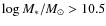 )
galaxies tend to have similar sizes than E/S0 galaxies.
At lower masses however they tend to lie between spirals and
spheroids.
)
galaxies tend to have similar sizes than E/S0 galaxies.
At lower masses however they tend to lie between spirals and
spheroids.
- The specific star formation rate measured with the
[OII]3727 line and stellar masses, shows that blue
E/S0 galaxies have similar SSFR values than normal
star-forming spirals. The outliers of this relation are galaxies more
massive than
 .
These outliers present SSFR characteristic of post-merger galaxies (
.
These outliers present SSFR characteristic of post-merger galaxies (
 ).
).
The confirmation of these hypothesis requires a detailed analysis of the internal kynematics of these objects to see if the physics is indeed different. In particular, 3D spectroscopy should be useful to get more details about their nature.
AcknowledgementsBased on zCOSMOS observations carried out using the Very Large Telescope at the ESO Paranal Observatory under Programme ID: LP175.A-0839. The Millennium Simulation databases used in this paper and the web application providing online access to them were constructed as part of the activities of the German Astrophysical Virtual Observatory. The authors would like to thank ESO for financial support.
References
- Abraham, R., van den Bergh, S., Glazebrook, K., et al. 1996, ApJS, 107, 1 [NASA ADS] [CrossRef] [Google Scholar]
- Abraham, R. G., Valdes, F., Yee, H. K. C., & van den Bergh, S. 1994, ApJ, 432, 75 [NASA ADS] [CrossRef] [Google Scholar]
- Adelman-McCarthy, J. K., Agüeros, M. A., Allam, S. S., et al. 2006, ApJS, 162, 38 [NASA ADS] [CrossRef] [Google Scholar]
- Aguerri, J. A. L., & Trujillo, I. 2002, MNRAS, 333, 633 [NASA ADS] [CrossRef] [Google Scholar]
- Aguerri, J. A. L., Balcells, M., & Peletier, R. F. 2001, A&A, 367, 428 [NASA ADS] [CrossRef] [EDP Sciences] [Google Scholar]
- Aguerri, J. A. L., Iglesias-Paramo, J., Vilchez, J. M., & Muñoz-Tuñón, C. 2004, AJ, 127, 1344 [NASA ADS] [CrossRef] [Google Scholar]
- Aguerri, J. A. L., Iglesias-Páramo, J., Vílchez, J. M., Muñoz-Tuñón, C., & Sánchez-Janssen, R. 2005, AJ, 130, 475 [NASA ADS] [CrossRef] [Google Scholar]
- Azzollini, R., Trujillo, I., & Beckman, J. E. 2008, ApJ, 684, 1026 [NASA ADS] [CrossRef] [Google Scholar]
- Baldry, I. K., Glazebrook, K., Brinkmann, J., et al. 2004, ApJ, 600, 681 [NASA ADS] [CrossRef] [Google Scholar]
- Bamford, S. P., Nichol, R. C., Baldry, I. K., et al. 2009, MNRAS, 393, 1324 [NASA ADS] [CrossRef] [Google Scholar]
- Barnes, J. E. 2002, MNRAS, 333, 481 [NASA ADS] [CrossRef] [Google Scholar]
- Benson, A. J., Bower, R. G., Frenk, C. S., et al. 2003, ApJ, 599, 38 [NASA ADS] [CrossRef] [Google Scholar]
- Binney, J. 1977, ApJ, 215, 483 [NASA ADS] [CrossRef] [Google Scholar]
- Blanton, M. R., Schlegel, D. J., Strauss, M. A., et al. 2005, AJ, 129, 2562 [NASA ADS] [CrossRef] [Google Scholar]
- Blumenthal, G. R., Faber, S. M., Primack, J. R., & Rees, M. J. 1984, Nature, 311, 517 [NASA ADS] [CrossRef] [Google Scholar]
- Bolzonella, M., Kovac, K., Pozzetti, L., et al. 2009, A&A, submitted [arXiv:0907.0013] [Google Scholar]
- Bower, R. G., Benson, A. J., Malbon, R., et al. 2006, MNRAS, 370, 645 [NASA ADS] [CrossRef] [Google Scholar]
- Brook, C. B., Kawata, D., Martel, H., Gibson, B. K., & Bailin, J. 2006, ApJ, 639, 126 [NASA ADS] [CrossRef] [Google Scholar]
- Bundy, K., Ellis, R. S., & Conselice, C. J. 2005, ApJ, 625, 621 [NASA ADS] [CrossRef] [Google Scholar]
- Capak, P., Aussel, H., Ajiki, M., et al. 2007, ApJS, 172, 99 [NASA ADS] [CrossRef] [Google Scholar]
- Cattaneo, A., Dekel, A., Devriendt, J., Guiderdoni, B., & Blaizot, J. 2006, MNRAS, 370, 1651 [NASA ADS] [CrossRef] [Google Scholar]
- Cattaneo, A., Dekel, A., Faber, S. M., & Guiderdoni, B. 2008, MNRAS, 389, 567 [NASA ADS] [CrossRef] [Google Scholar]
- Cimatti, A., Daddi, E., & Renzini, A. 2006, A&A, 453, L29 [NASA ADS] [CrossRef] [EDP Sciences] [Google Scholar]
- Cole, S., Lacey, C. G., Baugh, C. M., & Frenk, C. S. 2000, MNRAS, 319, 168 [NASA ADS] [CrossRef] [Google Scholar]
- Conselice, C. J., Rajgor, S., & Myers, R. 2008, MNRAS, 386, 909 [NASA ADS] [CrossRef] [Google Scholar]
- Conselice, C. J., Yang, C., & Bluck, A. F. L. 2009, MNRAS, 394, 1956 [NASA ADS] [CrossRef] [Google Scholar]
- Cowie, L. L., Songaila, A., Hu, E. M., & Cohen, J. G. 1996, AJ, 112, 839 [Google Scholar]
- Cox, T. J., Primack, J., Jonsson, P., & Somerville, R. S. 2004, ApJ, 607, L87 [NASA ADS] [CrossRef] [Google Scholar]
- de Jong, R. S., Simard, L., Davies, R. L., et al. 2004, MNRAS, 355, 1155 [NASA ADS] [CrossRef] [Google Scholar]
- De Lucia, G., Springel, V., White, S. D. M., Croton, D., & Kauffmann, G. 2006, MNRAS, 366, 499 [NASA ADS] [CrossRef] [Google Scholar]
- Dekel, A., & Birnboim, Y. 2006, MNRAS, 368, 2 [NASA ADS] [CrossRef] [Google Scholar]
- Eliche-Moral, M. C., Balcells, M., Aguerri, J. A. L., & González-García, A. C. 2006, A&A, 457, 91 [NASA ADS] [CrossRef] [EDP Sciences] [Google Scholar]
- Faber, S. M., Willmer, C. N. A., Wolf, C., et al. 2007, ApJ, 665, 265 [NASA ADS] [CrossRef] [Google Scholar]
- Fabian, A. C. 1999, MNRAS, 308, L39 [NASA ADS] [CrossRef] [Google Scholar]
- Ferreras, I., Lisker, T., Pasquali, A., & Kaviraj, S. 2009, MNRAS, 395, 554 [NASA ADS] [CrossRef] [Google Scholar]
- Governato, F., Willman, B., Mayer, L., et al. 2007, MNRAS, 374, 1479 [NASA ADS] [CrossRef] [Google Scholar]
- Guzman, R., Gallego, J., Koo, D. C., et al. 1997, ApJ, 489, 559 [NASA ADS] [CrossRef] [Google Scholar]
- Hammer, F., Gruel, N., Thuan, T. X., Flores, H., & Infante, L. 2001, ApJ, 550, 570 [NASA ADS] [CrossRef] [Google Scholar]
- Hammer, F., Flores, H., Yang, Y. B., et al. 2009, A&A, 496, 381 [NASA ADS] [CrossRef] [EDP Sciences] [Google Scholar]
- Hernquist, L., & Mihos, J. C. 1995, ApJ, 448, 41 [NASA ADS] [CrossRef] [Google Scholar]
- Huertas-Company, M., Rouan, D., Tasca, L., Soucail, G., & Le Fèvre, O. 2008, A&A, 478, 971 [NASA ADS] [CrossRef] [EDP Sciences] [Google Scholar]
- Huertas-Company, M., Tasca, L., Rouan, D., et al. 2009, A&A, 497, 743 [NASA ADS] [CrossRef] [EDP Sciences] [Google Scholar]
- Ilbert, O., Arnouts, S., McCracken, H. J., et al. 2006a, A&A, 457, 841 [NASA ADS] [CrossRef] [EDP Sciences] [Google Scholar]
- Ilbert, O., Lauger, S., Tresse, L., et al. 2006b, A&A, 453, 809 [NASA ADS] [CrossRef] [EDP Sciences] [Google Scholar]
- Kannappan, S. J. 2004, ApJ, 611, L89 [NASA ADS] [CrossRef] [MathSciNet] [Google Scholar]
- Kannappan, S. J., & Wei, L. H. 2008, in The Evolution of Galaxies Through the Neutral Hydrogen Window, ed. R. Minchin, & E. Momjian, Am. Inst. Phys. Conf. Ser., 1035, 163 [Google Scholar]
- Kannappan, S. J., Guie, J. M., & Baker, A. J. 2009, AJ, 138, 579 [NASA ADS] [CrossRef] [Google Scholar]
- Kanwar, A., Simard, L., Schade, D., & Gwyn, S. D. J. 2008, ApJ, 682, 907 [NASA ADS] [CrossRef] [Google Scholar]
- Kauffmann, G., Heckman, T. M., De Lucia, G., et al. 2006, MNRAS, 367, 1394 [NASA ADS] [CrossRef] [Google Scholar]
- Keres, D., Katz, N., Weinberg, D. H., & Davé, R. 2005, MNRAS, 363, 2 [NASA ADS] [CrossRef] [Google Scholar]
- King, A. 2003, ApJ, 596, L27 [NASA ADS] [CrossRef] [Google Scholar]
- Koekemoer, A. M., Aussel, H., Calzetti, D., et al. 2007, ApJS, 172, 196 [NASA ADS] [CrossRef] [Google Scholar]
- Le Fèvre, O., Abraham, R., Lilly, S. J., et al. 2000, MNRAS, 311, 565 [NASA ADS] [CrossRef] [Google Scholar]
- Lilly, S. J., LeBrun, V., Maier, C., et al. 2009, ApJS, 184, 218 [Google Scholar]
- Martig, M., Bournaud, F., Teyssier, R., & Dekel, A. 2009, ApJ, 707, 250 [NASA ADS] [CrossRef] [Google Scholar]
- Méndez-Abreu, J., Aguerri, J. A. L., Corsini, E. M., & Simonneau, E. 2008, A&A, 487, 555 [NASA ADS] [CrossRef] [EDP Sciences] [Google Scholar]
- Mihos, J. C., & Hernquist, L. 1996, ApJ, 464, 641 [NASA ADS] [CrossRef] [Google Scholar]
- Peng, C. Y., Ho, L. C., Impey, C. D., & Rix, H.-W. 2002, AJ, 124, 266 [NASA ADS] [CrossRef] [Google Scholar]
- Phillips, A. C., Guzman, R., Gallego, J., et al. 1997, ApJ, 489, 543 [NASA ADS] [CrossRef] [Google Scholar]
- Pozzetti, L., Bolzonella, M., Zucca, E., et al. 2009, A&A, submitted [arXiv:0907.5416] [Google Scholar]
- Puech, M., Hammer, F., Lehnert, M. D., & Flores, H. 2007, A&A, 466, 83 [NASA ADS] [CrossRef] [EDP Sciences] [Google Scholar]
- Rees, M. J., & Ostriker, J. P. 1977, MNRAS, 179, 541 [NASA ADS] [CrossRef] [Google Scholar]
- Robertson, B. E., & Bullock, J. S. 2008, ApJ, 685, L27 [NASA ADS] [CrossRef] [Google Scholar]
- Sanders, D. B., Salvato, M., Aussel, H., et al. 2007, ApJS, 172, 86 [Google Scholar]
- Schawinski, K., Lintott, C., Thomas, D., et al. 2009, MNRAS, 396, 818 [NASA ADS] [CrossRef] [Google Scholar]
- Scoville, N., Aussel, H., Brusa, M., et al. 2007, ApJS, 172, 1 [NASA ADS] [CrossRef] [Google Scholar]
- Silk, J., & Rees, M. J. 1998, A&A, 331, L1 [NASA ADS] [Google Scholar]
- Simard, L., Willmer, C. N. A., Vogt, N. P., et al. 2002, ApJS, 142, 1 [NASA ADS] [CrossRef] [Google Scholar]
- Springel, V., Di Matteo, T., & Hernquist, L. 2005a, ApJ, 620, L79 [NASA ADS] [CrossRef] [Google Scholar]
- Springel, V., White, S. D. M., Jenkins, A., et al. 2005b, Nature, 435, 629 [NASA ADS] [CrossRef] [PubMed] [Google Scholar]
- Strateva, I., Ivezic, Z., Knapp, G. R., et al. 2001, AJ, 122, 1861 [Google Scholar]
- Tasca, L. A. M., Kneib, J., Iovino, A., et al. 2009, A&A, 503, 379 [NASA ADS] [CrossRef] [EDP Sciences] [Google Scholar]
- Trujillo, I., & Aguerri, J. A. L. 2004, MNRAS, 355, 82 [NASA ADS] [CrossRef] [Google Scholar]
- Trujillo, I., Graham, A. W., & Caon, N. 2001, MNRAS, 326, 869 [NASA ADS] [CrossRef] [Google Scholar]
- van den Bergh, S., Abraham, R. G., Ellis, R. S., et al. 1996, AJ, 112, 359 [NASA ADS] [CrossRef] [Google Scholar]
- White, S. D. M., & Rees, M. J. 1978, MNRAS, 183, 341 [NASA ADS] [CrossRef] [Google Scholar]
- Wyithe, J. S. B., & Loeb, A. 2003, ApJ, 595, 614 [NASA ADS] [CrossRef] [Google Scholar]
- Zamojski, M. A., Schiminovich, D., Rich, R. M., et al. 2007, ApJS, 172, 468 [NASA ADS] [CrossRef] [Google Scholar]
Footnotes
All Tables
Table 1: Characteristic mass for different redshift bins.
All Figures
|
|
Figure 1: Stellar mass vs. redshift. Blue points are blue late-type galaxies and red diamonds are red early-type galaxies. Horizontal lines from bottom to top show the estimated mass completeness at z<0.55, z<0.8 and z<1.4 respectively. |
| Open with DEXTER | |
| In the text | |
|
|
Figure 2:
5'' |
| Open with DEXTER | |
| In the text | |
|
|
Figure 3: (U-R) rest-frame color - stellar mass diagrams for morphologically selected early-type galaxies ( top) and late-type galaxies (down) in three redshift bins. Colors indicate the rest-frame color based classification: objects with red templates ([T1-T20]) are shown in red and objects with blue templates ([T21-T38]) are shown in blue. |
| Open with DEXTER | |
| In the text | |
|
|
Figure 4: Fraction of blue early-type galaxies as a function of mass at different redshifts. Red line: 0.8<z<1.4, green line: 0.5<z<0.8 and blue line: 0.2<z<0.5. Vertical lines show the estimated mass completeness at the different redshift bins. Filled circles show the results from the Millenium simulation at all redshifts (see text for details). |
| Open with DEXTER | |
| In the text | |
|
|
Figure 5: Fractions of blue late-type (blue line) and red early-type galaxies (red line) in the three considered redshift bins as a function of the stellar mass. Dashed vertical lines show the estimated mass completeness at the corresponding redshift bin. |
| Open with DEXTER | |
| In the text | |
|
|
Figure 6:
|
| Open with DEXTER | |
| In the text | |
|
|
Figure 7: Radius-stellar mass relation at different redshifts. Red circles are red E/S0 galaxies, black points are blue late-type systems and filled blue circles are blue early-type galaxies. Vertical dashed lines show the threshold mass at different redshifts as computed in Sect. 4.2. Solid line indicates the best fit line for red E/S0 galaxies. |
| Open with DEXTER | |
| In the text | |
|
|
Figure 8: Specific star formation rate as a function of stellar mass in 3 redshift bins. Black dots are normal blue late-type galaxies and blue filled dots are blue early-type galaxies. Vertical dashed lines indicate the threshold mass. Solid line is the best fit to the spiral star-forming population and dashed line is the 3-sigma limit. |
| Open with DEXTER | |
| In the text | |
|
|
Figure 9: I-band magnitude versus half light radius. Blue filled circles are our blue early-type galaxies, empty red circles are red E/S0 and black dots are blue late-type galaxies. The solid line shows the limit used in Phillips et al. (1997) to define compact objects. |
| Open with DEXTER | |
| In the text | |
|
|
Figure 10: Morphological mixing of compact galaxies as a function of the stellar mass. Red line are passive early-type galaxies, blue line are blue early-type galaxies, black line blue late-type galaxies and green line red late-type galaxies. |
| Open with DEXTER | |
| In the text | |
|
|
Figure 11:
Evolution of number density of blue E/S0 in two mass bins.
Diamonds are blue E/S0 with |
| Open with DEXTER | |
| In the text | |
|
|
Figure 12: R-band rest-frame surface brightness vs. stellar mass for our sample compared with the SDSS DR4 sample. Each column shows a different redshift range, i.e. from left to right: 0.2<z<0.55, 0.55<z<0.8 and 0.8<z<1.4. Contours show in all sub-figures the location (20 galaxies iso-contour) of local galaxies (red dashed contours are early-type galaxies and blue solid contours are late-type galaxies). Over plotted are galaxies in our sample, top: blue E/S0, middle: red E/S0, and bottom: blue late-type systems. Dashed horizontal lines indicate the threshold mass and the solid line are our completeness limit. Arrows show typical movements in the plane caused by fading or disk rebuilding activity. |
| Open with DEXTER | |
| In the text | |
Copyright ESO 2010
Current usage metrics show cumulative count of Article Views (full-text article views including HTML views, PDF and ePub downloads, according to the available data) and Abstracts Views on Vision4Press platform.
Data correspond to usage on the plateform after 2015. The current usage metrics is available 48-96 hours after online publication and is updated daily on week days.
Initial download of the metrics may take a while.