| Issue |
A&A
Volume 515, June 2010
|
|
|---|---|---|
| Article Number | A48 | |
| Number of page(s) | 15 | |
| Section | Cosmology (including clusters of galaxies) | |
| DOI | https://doi.org/10.1051/0004-6361/200912924 | |
| Published online | 08 June 2010 | |
Simulations of the cosmic infrared and submillimeter background for future large surveys
II. Removing the low-redshift contribution to the anisotropies using stacking
N. Fernandez-Conde - G. Lagache - J.-L. Puget - H. Dole
Institut d'Astrophysique Spatiale (IAS), Bât. 121, Université Paris-Sud 11 and CNRS (UMR 8617), 91405 Orsay, France
Received 17 July 2009 / Accepted 17 January 2010
Abstract
Context. Herschel and Planck are surveying the sky at
unprecedented angular scales and sensitivities over large areas. But
both experiments are limited by source confusion in the submillimeter.
The high confusion noise in particular restricts the study of the
clustering properties of the sources that dominate the cosmic infrared
background. At these wavelengths, it is more appropriate to consider
the statistics of the unresolved component. In particular, high
clustering will contribute in excess of Poisson noise in the power
spectra of CIB anisotropies.
Aims. These power spectra contain contributions from sources at
all redshift. We show how the stacking technique can be used to
separate the different redshift contributions to the power spectra.
Methods. We use simulations of CIB representative of realistic
Spitzer, Herschel, Planck, and SCUBA-2 observations. We stack the
24 ![]() m
sources in longer wavelengths maps to measure mean colors per redshift
and flux bins. The information retrieved on the mean spectral energy
distribution obtained with the stacking technique is then used to clean
the maps, in particular to remove the contribution of low-redshift
undetected sources to the anisotropies.
m
sources in longer wavelengths maps to measure mean colors per redshift
and flux bins. The information retrieved on the mean spectral energy
distribution obtained with the stacking technique is then used to clean
the maps, in particular to remove the contribution of low-redshift
undetected sources to the anisotropies.
Results. Using the stacking, we measure the mean flux of populations 4 to 6 times fainter than the total noise at 350 ![]() m at redshifts z=1 and z=2, respectively, and as faint as 6 to 10 times fainter than the total noise at 850
m at redshifts z=1 and z=2, respectively, and as faint as 6 to 10 times fainter than the total noise at 850 ![]() m at the same redshifts. In the deep Spitzer fields, the detected 24
m at the same redshifts. In the deep Spitzer fields, the detected 24 ![]() m sources up to
m sources up to ![]() contribute significantly to the submillimeter anisotropies. We show that the method provides excellent (using COSMOS 24
contribute significantly to the submillimeter anisotropies. We show that the method provides excellent (using COSMOS 24 ![]() m data) to good (using SWIRE 24
m data) to good (using SWIRE 24 ![]() m data) removal of the z<2 (COSMOS) and z<1 (SWIRE) anisotropies.
m data) removal of the z<2 (COSMOS) and z<1 (SWIRE) anisotropies.
Conclusions. Using this cleaning method, we then hope to have a
set of large maps dominated by high redshift galaxies for galaxy
evolution study (e.g., clustering, luminosity density).
Key words: methods: statistical - infrared: galaxies - galaxies: evolution
1 Introduction
The first observational evidence of the cosmic infrared background (CIB) was
reported by Puget et al. (1996) and confirmed by Fixsen et al. (1998) and Hauser et al. (1998).
The CIB is composed of the relic emission at infrared wavelengths
of the formation and evolution of galaxies and consists of contributions
from infrared starburst galaxies and to a lesser degree from active galactic
nuclei. Deep cosmological surveys of this background
have been carried out with ISO (see Elbaz 2005; Genzel & Cesarsky 2000, for reviews)
mainly at 15 ![]() m
with ISOCAM (e.g., Elbaz et al. 2002); at 90 and 170
m
with ISOCAM (e.g., Elbaz et al. 2002); at 90 and 170 ![]() m
with ISOPHOT (e.g., Dole et al. 2001); with Spitzer at 24,
70, and 160
m
with ISOPHOT (e.g., Dole et al. 2001); with Spitzer at 24,
70, and 160 ![]() m (e.g., Dole et al. 2004; Papovich et al. 2004)
and with ground-based instruments SCUBA (e.g., Blain et al. 2002), LABOCA
(e.g., Beelen et al. 2008), and MAMBO (e.g., Bertoldi et al. 2000) at 850, 870, and 1300
m (e.g., Dole et al. 2004; Papovich et al. 2004)
and with ground-based instruments SCUBA (e.g., Blain et al. 2002), LABOCA
(e.g., Beelen et al. 2008), and MAMBO (e.g., Bertoldi et al. 2000) at 850, 870, and 1300 ![]() m
respectively. The balloon-borne experiment BLAST performed the first deep extragalactic surveys at wavelengths 250-500
m
respectively. The balloon-borne experiment BLAST performed the first deep extragalactic surveys at wavelengths 250-500 ![]() m capable of measuring large numbers of star-forming
galaxies, and their contributions to the CIB (Devlin et al. 2009).
These surveys allowed us to obtain a far clearer understanding
of the CIB and its sources (see Lagache et al. 2005, for a general review) but many questions remain unanswered such as
the evolution of their spatial distribution with redshift.
m capable of measuring large numbers of star-forming
galaxies, and their contributions to the CIB (Devlin et al. 2009).
These surveys allowed us to obtain a far clearer understanding
of the CIB and its sources (see Lagache et al. 2005, for a general review) but many questions remain unanswered such as
the evolution of their spatial distribution with redshift.
The spatial distribution of infrared galaxies as a function
of redshift is a key component of the scenario of galaxy formation and evolution.
However, its study
has been hampered by high confusion and instrumental noise
and/or by the small size of the fields of observation.
Tentative studies, with a small number of sources at 850 ![]() m
(Blain et al. 2004), found evidence of a relationship
between submillimeter galaxies and the formation of massive galaxies
in dense environments.
Works by Farrah et al. (2006) and Magliocchetti et al. (2008)
measured a strong clustering of ultra luminous infrared galaxies
(ULIRG) detected with Spitzer at high redshifts.
Alternatively, the infrared background anisotropies could also
provide information about the correlation between the sources of the
CIB and dark matter (Haiman & Knox 2000; Knox et al. 2001; Amblard & Cooray 2007),
and its redshift evolution.
Lagache et al. (2007) and Viero et al. (2009) reported the detection of a correlated component
in the background anisotropies using Spitzer/MIPS (160
m
(Blain et al. 2004), found evidence of a relationship
between submillimeter galaxies and the formation of massive galaxies
in dense environments.
Works by Farrah et al. (2006) and Magliocchetti et al. (2008)
measured a strong clustering of ultra luminous infrared galaxies
(ULIRG) detected with Spitzer at high redshifts.
Alternatively, the infrared background anisotropies could also
provide information about the correlation between the sources of the
CIB and dark matter (Haiman & Knox 2000; Knox et al. 2001; Amblard & Cooray 2007),
and its redshift evolution.
Lagache et al. (2007) and Viero et al. (2009) reported the detection of a correlated component
in the background anisotropies using Spitzer/MIPS (160 ![]() m) and BLAST (250, 350,
and 500
m) and BLAST (250, 350,
and 500 ![]() m) data. These authors found that star formation is highly biased at z > 0.8. The strong evolution
of the bias parameter with redshift, caused by the shifting
of star formation to more massive halos with increasing
redshift, infers that environmental effects influence
the vigorous star formation.
m) data. These authors found that star formation is highly biased at z > 0.8. The strong evolution
of the bias parameter with redshift, caused by the shifting
of star formation to more massive halos with increasing
redshift, infers that environmental effects influence
the vigorous star formation.
To improve our understanding of the formation and evolution of galaxies using
CIB anisotropies, we need more information about the redshift of the sources contributing to the
CIB. We also need a method that allows to go deeper than the confusion noise level. In this context,
an invaluable tool is the stacking technique, which allows a statistical
study of groups of sources that cannot be detected individually at a given wavelength. Its requires
the knowledge of the positions of the sources being ``stacked''
as inferred from their individual detection at another wavelength. This knowledge
is then used to stack the signal of the sources at the wavelength
at which they cannot be detected individually. Since the signal of the
sources increases with the number of sources N and the noise (if
Gaussian) increases with ![]() ,
the signal-to-noise ratio
will increase with
,
the signal-to-noise ratio
will increase with ![]() .
For an additional description of the basics of stacking techniques we
refer to for example Dole et al. (2006) and Marsden et al. (2009).
.
For an additional description of the basics of stacking techniques we
refer to for example Dole et al. (2006) and Marsden et al. (2009).
Stacking was used to measure the contribution
of 24 ![]() m galaxies to the background at 70 and 160
m galaxies to the background at 70 and 160 ![]() m using
MIPS data (Dole et al. 2006). Contribution from galaxies
down to 60
m using
MIPS data (Dole et al. 2006). Contribution from galaxies
down to 60 ![]() Jy at 24
Jy at 24 ![]() m is at least 79% of the 24
m is at least 79% of the 24 ![]() m,
and 80% of the 70 and 160
m,
and 80% of the 70 and 160 ![]() m backgrounds, respectively. At longer wavelengths
studies used this technique to determine the contribution
of populations selected in the near- and mid-infrared to the FIRB (far-infrared background) background:
3.6
m backgrounds, respectively. At longer wavelengths
studies used this technique to determine the contribution
of populations selected in the near- and mid-infrared to the FIRB (far-infrared background) background:
3.6 ![]() m selected sources to the 850
m selected sources to the 850 ![]() m background (Wang et al. 2006)
and 8
m background (Wang et al. 2006)
and 8 ![]() m and 24
m and 24 ![]() m selected sources to the 850
m selected sources to the 850 ![]() m
and 450
m
and 450 ![]() m backgrounds (Serjeant et al. 2008; Dye et al. 2006).
Finally, Marsden et al. (2009) measured total submillimeter intensities associated with all 24
m backgrounds (Serjeant et al. 2008; Dye et al. 2006).
Finally, Marsden et al. (2009) measured total submillimeter intensities associated with all 24 ![]() m
sources
that are consistent with 24 micron-selected galaxies generating
the full intensity of the FIRB. Similar studies with Planck and
Herschel will provide even more evidence about the nature of the FIRB
sources.
m
sources
that are consistent with 24 micron-selected galaxies generating
the full intensity of the FIRB. Similar studies with Planck and
Herschel will provide even more evidence about the nature of the FIRB
sources.
Theoretically, a stacking technique also could be used to study
the mean SED (spectral energy distribution) of the stacked
sources (e.g., Zheng et al. 2007).
The main potential limitations would be caused by
the errors in the redshifts of the sources and an
insufficiently large number of sources to stack per redshift bin.
The observation of sufficiently large fields to which the technique can be applied is now
assured by the to Spitzer legacy surveys FIDEL, COSMOS, and SWIRE![]() and Planck and Herschel surveys.
Advances in the measurement of the redshift have also been
accomplished, although for very small fields for
sources up to
and Planck and Herschel surveys.
Advances in the measurement of the redshift have also been
accomplished, although for very small fields for
sources up to ![]() (e.g. Caputi et al. 2006), and for the
larger COSMOS fields up to
(e.g. Caputi et al. 2006), and for the
larger COSMOS fields up to ![]() with very high accuracy (Ilbert et al. 2009). Future
surveys are planned to measure the redshifts
in larger fields such as the dark energy survey (DES
with very high accuracy (Ilbert et al. 2009). Future
surveys are planned to measure the redshifts
in larger fields such as the dark energy survey (DES![]() ) or the GAMA
spectroscopic survey (e.g. Baldry et al. 2008).
) or the GAMA
spectroscopic survey (e.g. Baldry et al. 2008).
The difficulties in separating the contribution to the signal coming from different redshifts have handicapped the study of CIB anisotropies. However, once the mean SEDs of infrared galaxies per redshift bin are obtained we can use this information to analyze CIB anisotropies. The SEDs obtained with the stacking technique can be used to ``clean'' the low-redshift anisotropies (or at least a significant part of them) from the CIB maps. This can be performed by subtracting the undetected low-redshift (z<1-2) populations from the maps using their mean colors and thus build maps dominated by sources at higher redshifts. This also facilitates the study of the evolution of large-scale structures at high redshift by removing the noise coming from low redshifts.
In this paper, we use the simulations and catalogs presented in
Fernandez-Conde et al. (2008)![]() to study the limitations of stacking techniques in CIB anisotropy analysis.
We stack 24
to study the limitations of stacking techniques in CIB anisotropy analysis.
We stack 24 ![]() m sources detected with MIPS in Planck, Herschel, and SCUBA-2 simulated observations.
The catalogs and maps were created for
different levels of bias between the fluctuations of infrared galaxy emissivities and the dark matter density field.
We use a bias b=1.5, which is very close to that measured by Lagache et al. (2007).
m sources detected with MIPS in Planck, Herschel, and SCUBA-2 simulated observations.
The catalogs and maps were created for
different levels of bias between the fluctuations of infrared galaxy emissivities and the dark matter density field.
We use a bias b=1.5, which is very close to that measured by Lagache et al. (2007).
The paper is organized as follows. In Sect. 2, we
explain the method used to study the capabilities of the stacking once the redshift of the sources is known. Section 3 details the elements that limit the accuracy of the stacking technique. In Sect. 4, we test the
technique for studying the mean SEDs of galaxies. In Sect. 5, the
feasibility of using information about the SEDs to clean the
observations of low-redshift anisotropies is studied. The results are summarized
in Sect. 6. Throughout this paper, the cosmological
parameters are assumed to be
![]() .
For the dark-matter linear clustering, we set the normalization to be
.
For the dark-matter linear clustering, we set the normalization to be
![]() .
.
2 Description of the method
Dole et al. (2006) considered every MIPS 24 ![]() m source in selected fields
with fluxes >60
m source in selected fields
with fluxes >60 ![]() Jy and then sorted the 24
Jy and then sorted the 24 ![]() m
sources by decreasing flux at 24
m
sources by decreasing flux at 24 ![]() m (hereafter S24).
The sources were placed in 20 bins of increasing flux density. These
bins were of equal logarithmic width
m (hereafter S24).
The sources were placed in 20 bins of increasing flux density. These
bins were of equal logarithmic width
![]() ,
except for the bin corresponding to the brightest flux, to
take all the bright sources. They then corrected the average flux obtained
by stacking each S24 bin for incompleteness using the correction
of Papovich et al. (2004). This allowed them to determine lower limits
to the CIB at 70
,
except for the bin corresponding to the brightest flux, to
take all the bright sources. They then corrected the average flux obtained
by stacking each S24 bin for incompleteness using the correction
of Papovich et al. (2004). This allowed them to determine lower limits
to the CIB at 70 ![]() m and 160
m and 160 ![]() m, and to find the contribution from galaxies
down to 60
m, and to find the contribution from galaxies
down to 60 ![]() Jy at 24
Jy at 24 ![]() m to be at least 79% of the 24
m to be at least 79% of the 24 ![]() m,
and 80% of the 70 and 160
m,
and 80% of the 70 and 160 ![]() m backgrounds.
m backgrounds.
While these measurements of the total flux are useful for estimating
the overall energy emitted by these populations (see also Marsden et al. 2009),
it does little to improve our knowledge of individual
sources. To use the average flux efficiently we have to decrease the
dispersion in the individual fluxes (at the long wavelength) around the average flux of the
population. We can do this by separating large populations of sources
into smaller and more homogeneous SED populations.
One of the main sources of flux dispersion is the measurement
of the mean flux using galaxies with very different redshifts.
The lack of accurate redshifts (up to ![]() )
across large fields has so far limited
the use of detailed redshift information in stacking analysis.
Because of this, the fluxes of sources with different SEDs are averaged together
and the mean flux is a poor estimator of the fluxes of individual
sources. However advances in the measurement of the redshifts are expected in the coming years
with the new generation of spectroscopic and photometric redshift surveys such as
GAMA (e.g. Baldry et al. 2008), (Big-)BOSS
)
across large fields has so far limited
the use of detailed redshift information in stacking analysis.
Because of this, the fluxes of sources with different SEDs are averaged together
and the mean flux is a poor estimator of the fluxes of individual
sources. However advances in the measurement of the redshifts are expected in the coming years
with the new generation of spectroscopic and photometric redshift surveys such as
GAMA (e.g. Baldry et al. 2008), (Big-)BOSS![]() ,
DES
,
DES![]() .
We developed a method that assumes that redshifts are known and investigated
the limitations of stacking techniques caused by the uncertainties in the redshifts.
We assessed the dispersion in the fluxes
of individual sources with different redshift errors and the influence of this dispersion on the
quality of the results using our
simulations since this information will not be available in the real
observations.
.
We developed a method that assumes that redshifts are known and investigated
the limitations of stacking techniques caused by the uncertainties in the redshifts.
We assessed the dispersion in the fluxes
of individual sources with different redshift errors and the influence of this dispersion on the
quality of the results using our
simulations since this information will not be available in the real
observations.
2.1 Stacking technique
We used our simulations to study the limitations of the stacking technique using 24 ![]() m MIPS
sources in Planck, Herschel, and SCUBA-2 observations. The choice of
this wavelength (24
m MIPS
sources in Planck, Herschel, and SCUBA-2 observations. The choice of
this wavelength (24 ![]() m) is motivated by several reasons. Firstly,
24
m) is motivated by several reasons. Firstly,
24 ![]() m is a good tracer of infrared galaxies (unlike e.g., near-infrared
detections). Secondly, 24
m is a good tracer of infrared galaxies (unlike e.g., near-infrared
detections). Secondly, 24 ![]() m-selected galaxies emit the bulk of the CIB up
to at least 500
m-selected galaxies emit the bulk of the CIB up
to at least 500 ![]() m (Dole et al. 2006; Marsden et al. 2009). Thirdly, 24
m (Dole et al. 2006; Marsden et al. 2009). Thirdly, 24 ![]() m Spitzer
observations provide large and deep surveys, with redshift distribution
of its sources extending up to redshift
m Spitzer
observations provide large and deep surveys, with redshift distribution
of its sources extending up to redshift ![]() .
The schematic description of our stacking process follows. The only
requirements are knowledge of both the redshifts of the
sources and their fluxes at 24
.
The schematic description of our stacking process follows. The only
requirements are knowledge of both the redshifts of the
sources and their fluxes at 24 ![]() m.
m.
The detected sources at 24 ![]() m will be characterized by two parameters
S24 and z.
We first remove from the long wavelength map (hereafter
m will be characterized by two parameters
S24 and z.
We first remove from the long wavelength map (hereafter ![]() map)
the sources detected individually, using the criteria described in
Fernandez-Conde et al. (2008). These sources are no longer considered in
the discussion, so whenever we refer to sources
we refer to those detected at 24
map)
the sources detected individually, using the criteria described in
Fernandez-Conde et al. (2008). These sources are no longer considered in
the discussion, so whenever we refer to sources
we refer to those detected at 24 ![]() m with
S24 greater than the detection threshold and not those detected
individually in the
m with
S24 greater than the detection threshold and not those detected
individually in the ![]() map.
The sources are then distributed into redshift bins.
The width of the redshift bins have to be optimized for each observation.
These bins cover the redshift interval between z=0 and
map.
The sources are then distributed into redshift bins.
The width of the redshift bins have to be optimized for each observation.
These bins cover the redshift interval between z=0 and
![]() ,
where
,
where ![]() is chosen depending on the goals of the work
is chosen depending on the goals of the work![]() . We stack independently the sources in each redshift slice. For the sources in a given redshift slice i (
. We stack independently the sources in each redshift slice. For the sources in a given redshift slice i (
![]() ), the process
of detection is as follows:
), the process
of detection is as follows:
- 1.
- Firstly, we order the sources by decreasing S24.
We start by stacking in the
 map the sub-images of the two
sources with higher S24
(that have not been detected individually).
Then we measure the signal-to-noise ratio of the resulting image. A
detection
is achieved when the signal-to-noise ratio is higher than a certain
detection threshold. This detection threshold is optimized for
different
observations. For the cases discussed in this paper, we use a
detection threshold of three. If we do not achieve a detection we stack
more sources (always selecting the next brighter sources at 24
map the sub-images of the two
sources with higher S24
(that have not been detected individually).
Then we measure the signal-to-noise ratio of the resulting image. A
detection
is achieved when the signal-to-noise ratio is higher than a certain
detection threshold. This detection threshold is optimized for
different
observations. For the cases discussed in this paper, we use a
detection threshold of three. If we do not achieve a detection we stack
more sources (always selecting the next brighter sources at 24  m)
m)![[*]](/icons/foot_motif.png) .
This is done until we attain the required signal-to-noise ratio.
.
This is done until we attain the required signal-to-noise ratio.
- 2.
- Once a detection is achieved, we assign to all sources stacked together a flux equal to the total flux measured in the stacked image divided by the number of sources.
- 3.
- After detection, we restart the process starting from the brightest sources that we have not yet stacked.
- 4.
- Sometimes the last (and therefore faintest) group of sources in the redshift slice is not successfully stacked by this algorithm because an insufficient number of faint sources remains to be stacked in this last iteration. To correct for this, we simply carry out the algorithm starting this time from the faintest sources and stacking progressively brighter sources until we achieve a detection. Although in this procedure the last two mean flux bins are not independent, the consequences in terms of systematic errors are negligible (since the sources affected are few, faint, and the relative error in the stacking is small).
-
 :
The mean
:
The mean
 of the sources
of the ith stacked population, where
of the sources
of the ith stacked population, where  is the reference
wavelength (here 24 m).
is the reference
wavelength (here 24 m).
- zSti: The mean redshift of the sources of the ith stacked population.
-
 :
The mean
:
The mean
 found for the sources
using the stacking technique for the ith stacked population.
found for the sources
using the stacking technique for the ith stacked population.
Redshift slice optimization:
Our algorithm assumes that sources at similar z and of similar S24 have similar characteristics at other wavelengths. Our best option to avoid substantial variance in2.2 Color smoothing
The algorithm discussed above is quite simplified because it
assumes that all sources detected in the same redshift bin
have the same color
![]() .
In contrast we would expect there to be a continuous
variation of
.
In contrast we would expect there to be a continuous
variation of
![]() with both
with both
![]() and z.
Following this assumption allows us to interpolate
values between detections at different
and z.
Following this assumption allows us to interpolate
values between detections at different
![]() for each
redshift slice.
A more complicated means of correction is to
smooth our predictions by interpolating
for each
redshift slice.
A more complicated means of correction is to
smooth our predictions by interpolating
![]() through the
grid formed by the set of points
through the
grid formed by the set of points
![]() found with the stacking algorithm described above for the whole
found with the stacking algorithm described above for the whole
![]() plane. We do this with the IDL function TRIGRID, which given data points
defined by the parameters
plane. We do this with the IDL function TRIGRID, which given data points
defined by the parameters
![]() and a triangulation of the planar set of points determined by
S24Stand zSt returns a regular grid of interpolated
and a triangulation of the planar set of points determined by
S24Stand zSt returns a regular grid of interpolated
![]() values. We tried both approaches and found that the differences between
the results for the two different smoothings is very small so from now on we use only the ``
values. We tried both approaches and found that the differences between
the results for the two different smoothings is very small so from now on we use only the ``
![]() smoothing''.
Figure 1a shows the fluxes at 350
smoothing''.
Figure 1a shows the fluxes at 350 ![]() m (with 1.5<z<1.6) before and after the
two dimensional smoothing. It shows the real fluxes of the sources (known from the simulations),
the recovered fluxes using the smoothing
technique, and the recovered fluxes without
smoothing. We can see that the smoothing greatly improves
the accuracy of the fluxes. After this
correction, the results are in very good agreement with the input fluxes.
m (with 1.5<z<1.6) before and after the
two dimensional smoothing. It shows the real fluxes of the sources (known from the simulations),
the recovered fluxes using the smoothing
technique, and the recovered fluxes without
smoothing. We can see that the smoothing greatly improves
the accuracy of the fluxes. After this
correction, the results are in very good agreement with the input fluxes.
![\begin{figure}
\par\includegraphics[width=6.5cm,clip]{12924_Plot1a}\par\includegraphics[width=6.5cm,clip]{12924_Plot1b}
\end{figure}](/articles/aa/full_html/2010/07/aa12924-09/img53.png)
|
Figure 1:
Top: input fluxes of the sources in the redshift slice 1.5<z<1.6
(solid line) together with estimates of the fluxes of the sources using
the smoothing technique (dashed line) and estimates of the fluxes of
the sources without smoothing (diamond). Bottom: the same but zoomed for
|
| Open with DEXTER | |
3 Limitations of the method
We now test the limitations of the method related to
the difficulties we expect to
face when real data are analyzed (e.g., intrinsic dispersion in the colors of the sources,
errors in the measurement of the fluxes and in redshifts, clustering)![]() .
To illustrate the limitations, in this section we use the simulations
at 350
.
To illustrate the limitations, in this section we use the simulations
at 350 ![]() m. We reached the same conclusions using other
far-infrared and submillimeter wavelengths. The size of the redshift slices that divide the
S24-z space was chosen to be dz=0.1;
wider redshift slices would stack together sources with very different
fluxes; smaller redshift slices led to too low signal-to-noise ratios.
m. We reached the same conclusions using other
far-infrared and submillimeter wavelengths. The size of the redshift slices that divide the
S24-z space was chosen to be dz=0.1;
wider redshift slices would stack together sources with very different
fluxes; smaller redshift slices led to too low signal-to-noise ratios.
Two different Spitzer surveys are used, COSMOS and SWIRE. COSMOS
is a deep observation with a completeness of ![]() 100%
up to
100%
up to
![]() Jy (Sanders et al. 2007).
It allows
us to test the stacking of faint sources. COSMOS covers a smaller field
than SWIRE (2 sq. deg. versus 50 sq. deg.) hence its stacking
measurements are less accurate for bright sources. Thus we also use the
much larger SWIRE survey (Lonsdale et al. 2004), which is less deep (
Jy (Sanders et al. 2007).
It allows
us to test the stacking of faint sources. COSMOS covers a smaller field
than SWIRE (2 sq. deg. versus 50 sq. deg.) hence its stacking
measurements are less accurate for bright sources. Thus we also use the
much larger SWIRE survey (Lonsdale et al. 2004), which is less deep (
![]() Jy)
but covers
Jy)
but covers ![]() 25 times more area
25 times more area![]() .
We analyze the stacking of 24
.
We analyze the stacking of 24 ![]() m sources
for two study cases: observations in the far-infrared with Herschel
at 350
m sources
for two study cases: observations in the far-infrared with Herschel
at 350 ![]() m and (in the next section) observations in the submillimeter with Planck and SCUBA-2 at 850
m and (in the next section) observations in the submillimeter with Planck and SCUBA-2 at 850 ![]() m.
The characteristics of the Herschel/SPIRE, Planck/HFI, and SCUBA-2 observations are the following:
m.
The characteristics of the Herschel/SPIRE, Planck/HFI, and SCUBA-2 observations are the following:
Stacking in the COSMOS field:
- Detection limit:
 Jy at
Jy at  m.
m.
- Size of the field: 2 sq. deg.
- Linear bias: b=1.5.
- Type of observation with Herschel: 350 m ``Deep'' (with 1
 mJy).
mJy).
- Type of observation with SCUBA-2: 850 m (with 1
 mJy).
mJy).
Stacking in the SWIRE fields:
- Detection limit:
 Jy at 24
 m.
m.
- Size of the field: 50 sq. deg.
- Linear bias: b=1.5.
- Type of observation with Herschel: 350
 m ``deep'' (with 1
mJy).
m ``deep'' (with 1
mJy).
- Type of observation with SCUBA-2 and Planck: 850m (with 1 mJy and
1
 mJy - see Table 4 from Fernandez-Conde et al. 2008- respectively).
3.1 Cold and starburst populations
Figure 2 shows the
histograms of the fluxes at 350 ![]() m for a stacking box with 0.5<z<0.6 and
0.5<S24<1 mJy.
The main source of error in the estimate of the fluxes for this case would not be the dispersion in either S24or z but the presence of two different populations, which are indistinguishable
using observations at shorter wavelengths. These two populations are
the starburst and the normal (cold) populations described in Lagache et al. (2003).
Figure 3 shows the number of starburst and normal
sources as a function of z for sources with
m for a stacking box with 0.5<z<0.6 and
0.5<S24<1 mJy.
The main source of error in the estimate of the fluxes for this case would not be the dispersion in either S24or z but the presence of two different populations, which are indistinguishable
using observations at shorter wavelengths. These two populations are
the starburst and the normal (cold) populations described in Lagache et al. (2003).
Figure 3 shows the number of starburst and normal
sources as a function of z for sources with
![]() Jy,
0.27<S24<1 mJy, and S24>1 mJy. For the three afore mentioned cases, the cold sources
are the dominant population for
z<0.8, z<0.6, and z<0.5 respectively.
There are no effective ways of separating these two populations, and this will cause poor estimates of
the mean colors of each population. This is particularly
important when the number of sources of each type is approximately equal. This
is because we add together two populations of very different S350(cold sources
are in general brighter in the submillimeter than starburst sources at the same redshifts
and with similar S24).
When one of the populations dominates, this problem becomes negligible.
Jy,
0.27<S24<1 mJy, and S24>1 mJy. For the three afore mentioned cases, the cold sources
are the dominant population for
z<0.8, z<0.6, and z<0.5 respectively.
There are no effective ways of separating these two populations, and this will cause poor estimates of
the mean colors of each population. This is particularly
important when the number of sources of each type is approximately equal. This
is because we add together two populations of very different S350(cold sources
are in general brighter in the submillimeter than starburst sources at the same redshifts
and with similar S24).
When one of the populations dominates, this problem becomes negligible.
3.2 Errors caused by intrinsic dispersion in colors
Because of the lack of constraints on SEDs at long wavelengths and their
evolution with redshift,
the Lagache et al. (2004) model does not take into account that galaxies of the same
luminosity and redshift could have different
values of
![]() (apart from the distinction between
normal and starburst sources). To assess the effect of this
dispersion, we introduce a random Gaussian error into the flux estimated
with the stacking for each of the stacked sources. The errors that we
make using this procedure are equivalent to those that we would make
if we were to use a model with an intrinsic Gaussian dispersion in the
(apart from the distinction between
normal and starburst sources). To assess the effect of this
dispersion, we introduce a random Gaussian error into the flux estimated
with the stacking for each of the stacked sources. The errors that we
make using this procedure are equivalent to those that we would make
if we were to use a model with an intrinsic Gaussian dispersion in the
![]() of the sources. This type of error does not affect the results
for the mean of the sources but the average difference between this
mean and the fluxes of the individual sources. We test the effect on our results
for different levels of dispersion (measured
in terms of the standard deviation in the dispersion compared to the mean
flux of the sources). In Fig. 4, we can
see the histograms of the errors for a dispersion of
of the sources. This type of error does not affect the results
for the mean of the sources but the average difference between this
mean and the fluxes of the individual sources. We test the effect on our results
for different levels of dispersion (measured
in terms of the standard deviation in the dispersion compared to the mean
flux of the sources). In Fig. 4, we can
see the histograms of the errors for a dispersion of ![]() ,
,
![]() ,
,
![]() for
all sources with
for
all sources with
![]() Jy. As expected, the figure illustrates how
the histograms broaden with dispersion. For a standard deviation in
the errors of the fluxes associated with the stacking
Jy. As expected, the figure illustrates how
the histograms broaden with dispersion. For a standard deviation in
the errors of the fluxes associated with the stacking
![]() and
a standard deviation associated with the fluxes
and
a standard deviation associated with the fluxes
![]() ,
the
final standard deviation in our errors
,
the
final standard deviation in our errors
![]() would be
would be
![]() .
We do not analyze other statistical representations of this effect
(i.e., non-Gaussian intrinsic dispersion) since we do not have any
strong observational constraints.
.
We do not analyze other statistical representations of this effect
(i.e., non-Gaussian intrinsic dispersion) since we do not have any
strong observational constraints.
![\begin{figure}
\par\includegraphics[width=7.cm]{12924_Plot2a}
\end{figure}](/articles/aa/full_html/2010/07/aa12924-09/img73.png)
|
Figure 2:
Histogram of the fluxes at 350 |
| Open with DEXTER | |
![\begin{figure}
\par\includegraphics[width=4cm]{12924_Plot3a}\includegraphics[wid...
...space*{2cm}\includegraphics[width=4cm]{12924_Plot3c}\hspace*{2cm}}\end{figure}](/articles/aa/full_html/2010/07/aa12924-09/img74.png)
|
Figure 3:
Histograms of the number of cold (thin line) and starburst (thick line) sources per 24 |
| Open with DEXTER | |
3.3 Redshift uncertainty
The effect of redshift errors are difficult to evaluate. This is because they combine with the non-linear k-correction, making the variation in
![]() with z complex.
In Sect. 4, we study the effect of redshift errors
for two different relative errors
with z complex.
In Sect. 4, we study the effect of redshift errors
for two different relative errors
![]() and
and
![]() .
.
![\begin{figure}
\par\includegraphics[width=7cm]{12924_Plot4}
\end{figure}](/articles/aa/full_html/2010/07/aa12924-09/img77.png)
|
Figure 4:
Ratio of recovered fluxes from stacking (
|
| Open with DEXTER | |
3.4 Problematic areas of the S24-z space
Figure 5 shows the errors
in the estimate of the mean fluxes in the S24-zspace for a 350 ![]() m Herschel observation of the COSMOS field
with redshift errors
m Herschel observation of the COSMOS field
with redshift errors
![]() and
and
![]() .
For the estimates of the fluxes,
we can easily identify several problematic areas in the S24-z space.
These are: data points at very low redshifts (z<0.1),
the brightest sources because of small number statistics and the faintest sources because
of flux errors
.
For the estimates of the fluxes,
we can easily identify several problematic areas in the S24-z space.
These are: data points at very low redshifts (z<0.1),
the brightest sources because of small number statistics and the faintest sources because
of flux errors![]() .
.
Low z:
There are very few sources at z<0.1. This prevents the stacking from achieving high signal-to-noise ratio levels. This translates into large errors in the measurement of the mean fluxes for sources with z<0.1.Bright sources:
These sources are rare and we are therefore unable to reach signal-to-noise ratios as good as for fainter sources. We expect the results for bright sources to be better when the stacking technique is applied to larger fields (for example using the WISE survey Mainzer et al. 2005). We should keep this in mind when analyzing the results in our study cases.Faint sources:
Another shortcoming of the method is that the smoothing techniques cannot be applied to sources fainter than the stacked flux of the faintest bin. The best solution is to assume for the last point given by the stacking that all the sources have the same color, which is equivalent to assuming that their color is the same as that of the sources that are slightly brighter than them.![\begin{figure}
\par\mbox{\includegraphics[width=4.3cm]{12924_Plot5a}\includegrap...
...Plot5c}\hspace{0.2cm} \includegraphics[width=4.cm]{12924_Plot5d} }\end{figure}](/articles/aa/full_html/2010/07/aa12924-09/img81.png)
|
Figure 5:
Accuracy in the mean recovered fluxes at 350 |
| Open with DEXTER | |
4 Application of the method
We now verify the accuracy of the method with realistic
simulations of observations including redshift errors and by using existing observations at 24 ![]() m with Spitzer.
m with Spitzer.
4.1 Stacking Herschel data in the far-infrared: 350 m
We comment on the main issues and sources of error encountered
when stacking 24 ![]() m sources in Herschel/Spire observations
at 350
m sources in Herschel/Spire observations
at 350 ![]() m and considering a detection threshold of
3
m and considering a detection threshold of
3![]() .
We note that the difficulties faced by the stacking technique
at 250 and 500
.
We note that the difficulties faced by the stacking technique
at 250 and 500 ![]() m are similar.
We use a division in the z axis with redshift slices of dz=0.1.
We analyze the results for two redshift errors, an
optimistic one of
m are similar.
We use a division in the z axis with redshift slices of dz=0.1.
We analyze the results for two redshift errors, an
optimistic one of
![]() and a pessimistic one of
and a pessimistic one of
![]() .
This illustrates the degradation in the quality of the results with redshift error.
.
This illustrates the degradation in the quality of the results with redshift error.
Errors in individual recovered fluxes:
Figure 6 shows the errors in the estimate of the fluxes of the sources with the stacking technique for redshifts 0<z<1 and 1<z<2 for an observation of the COSMOS field at 350![\begin{figure}
\par {\hspace*{4.5mm}\includegraphics[width=6.3cm]{12924_Plot6a}\...
...dth=6.3cm]{12924_Plot6c}\includegraphics[width=7.2cm]{12924_Plot6d}
\end{figure}](/articles/aa/full_html/2010/07/aa12924-09/img83.png)
|
Figure 6:
Relative errors in recovered fluxes for individual sources at 350 |
| Open with DEXTER | |
Limit for faint sources:
Stacking in the COSMOS field allows the detection of sources as faint as![\begin{figure}
\par\includegraphics[width=6.5cm]{12924_Plot7a}\includegraphics[w...
...4_Plot7c}\includegraphics[width=6.5cm]{12924_Plot7d}
\vspace*{-4mm}
\end{figure}](/articles/aa/full_html/2010/07/aa12924-09/img87.png)
|
Figure 7:
Same as Fig. 6 but for an
observation at 350 |
| Open with DEXTER | |
Mean errors:
The final results for the fluxes and colors of the sources obtained using the stacking technique are compared with the real (input) values in Figs. 8 and 9. They are in very good agreement with the input fluxes (called real fluxes in the figures) but to obtain a clearer idea of the errors we show in Fig. 10 two plots of the mean flux relative error4.2 Stacking Planck and SCUBA-2 data at 850 m
When applying the same technique to Planck observations
at 850 ![]() m, we encounter a fundamental limitation
of the stacking technique. In the stacked image, we can discern two
contributions to the peak, one associated
with the stacked sources, which has the shape of the PSF, and another broader
peak around it which is associated with the sources correlated with the stacked
sources. The method works easily when the PSF width is much smaller
than the width of the correlation peak. However, this condition is
not fulfilled for Planck observations where the width of
the correlation signal around sources is not very different from the
width of the PSF. Furthermore, when stacking faint sources,
m, we encounter a fundamental limitation
of the stacking technique. In the stacked image, we can discern two
contributions to the peak, one associated
with the stacked sources, which has the shape of the PSF, and another broader
peak around it which is associated with the sources correlated with the stacked
sources. The method works easily when the PSF width is much smaller
than the width of the correlation peak. However, this condition is
not fulfilled for Planck observations where the width of
the correlation signal around sources is not very different from the
width of the PSF. Furthermore, when stacking faint sources,
![]() Jy, the signal associated with the correlations
is much stronger than that of the sources: it becomes impossible
to distinguish between the signal from the sources
being stacked and the signal from the clustering.
Figure 11 shows a cut of a
stacked image for very faint sources (
Jy, the signal associated with the correlations
is much stronger than that of the sources: it becomes impossible
to distinguish between the signal from the sources
being stacked and the signal from the clustering.
Figure 11 shows a cut of a
stacked image for very faint sources (
![]() Jy).
The figure shows the total signal, the
signal coming from both the clustering and the
sources. For these faint sources, we can see that
the signal from the clustering of the sources is more important
than that of the stacked sources and their FWHMs are very similar.
Several attempts were made to correct this problem. By far the
most effective solution is to use additional observations with
a narrower PSF at similar wavelengths to estimate the fraction of the
flux that is associated with the clustering. This method is described
hereafter. Another possible solution that does not rely on complementary observations is presented in Appendix A.
Jy).
The figure shows the total signal, the
signal coming from both the clustering and the
sources. For these faint sources, we can see that
the signal from the clustering of the sources is more important
than that of the stacked sources and their FWHMs are very similar.
Several attempts were made to correct this problem. By far the
most effective solution is to use additional observations with
a narrower PSF at similar wavelengths to estimate the fraction of the
flux that is associated with the clustering. This method is described
hereafter. Another possible solution that does not rely on complementary observations is presented in Appendix A.
![\begin{figure}
\par\includegraphics[width=4.cm, height=5.35cm]{12924_Plot8a}\includegraphics[width=4.cm, height=5.35cm]{12924_Plot8b}
\end{figure}](/articles/aa/full_html/2010/07/aa12924-09/img89.png)
|
Figure 8:
Left: real fluxes of the sources at 350 |
| Open with DEXTER | |
![\begin{figure}
\par\includegraphics[width=4.cm, height=5.35cm]{12924_Plot9a}\includegraphics[width=4.cm,clip]{12924_Plot9b}
\end{figure}](/articles/aa/full_html/2010/07/aa12924-09/img90.png)
|
Figure 9: Left: real S350/S24 flux ratio of the sources in the space S24-z. Right: S350/S24 flux ratio found by the smoothed stacking technique ( right). The colors correspond to different values of the ratio, while the vertical axis is S24 and the horizontal axis is the redshift bin. The S24-z space is divided linearly in z and logarithmically in S24. |
| Open with DEXTER | |
![\begin{figure}
\par\includegraphics[width=4.cm]{12924_Plot10a}\includegraphics[width=4.cm]{12924_Plot10b}
\end{figure}](/articles/aa/full_html/2010/07/aa12924-09/img91.png)
|
Figure 10: Same as Fig. 5 but with no redshift errors. |
| Open with DEXTER | |
![\begin{figure}
\par\includegraphics[width=7cm]{12924_Plot11}
\end{figure}](/articles/aa/full_html/2010/07/aa12924-09/img92.png)
|
Figure 11:
Lateral cut of a stacking image (Planck/HFI at 850 |
| Open with DEXTER | |
The problem caused by the clustering contribution to the flux measured
with Planck/HFI makes it difficult to use this instrument alone to
estimate the fluxes accurately . It is therefore necessary to
use observations with other instruments with smaller FWHM. In the far-infrared,
we could use Herschel (for the same channel as Planck at 350 ![]() m).
For the submillimeter observations, we will have to use ground-based submillimeter instruments
(e.g., future camera SCUBA-2 at 850
m).
For the submillimeter observations, we will have to use ground-based submillimeter instruments
(e.g., future camera SCUBA-2 at 850 ![]() m or LABOCA at 870
m or LABOCA at 870 ![]() m).
m).
4.2.1 SCUBA-2 observation of the COSMOS field at 850  m
m
We analyze here the stacking of sources in the COSMOS field observed
with SCUBA-2. SCUBA-2 will have a very good sensitivity; we use an
estimate of the noise for these observations of ![]() mJy, close to that specified in the SCUBA-2 webpage
mJy, close to that specified in the SCUBA-2 webpage![]() .
Because the signal of the sources at 850
.
Because the signal of the sources at 850 ![]() m is much fainter relative to the noise than with Herschel at 350
m is much fainter relative to the noise than with Herschel at 350 ![]() m,
we have to increase the size of the redshift bins to achieve
detections. We take the following boundaries for the redshift slices
0, 0.1,0.4,0.8,1.,1.2,1.5,1.8, and 2.2. We use the same detection threshold as that used for Herschel at 350
m,
we have to increase the size of the redshift bins to achieve
detections. We take the following boundaries for the redshift slices
0, 0.1,0.4,0.8,1.,1.2,1.5,1.8, and 2.2. We use the same detection threshold as that used for Herschel at 350 ![]() m (
m (
![]() ).
).
Figure 12
shows the errors in the estimate of individual fluxes of
850 ![]() m sources for
m sources for
![]() Jy and redshifts 1<z<2with redshift errors of
Jy and redshifts 1<z<2with redshift errors of
![]() % (top),
3% (middle), and 10% (bottom).
The results are poorer than those at 350
% (top),
3% (middle), and 10% (bottom).
The results are poorer than those at 350 ![]() m (Fig. 6).
This is because
the signal of the individual sources is weaker relative to the noise
at 850
m (Fig. 6).
This is because
the signal of the individual sources is weaker relative to the noise
at 850 ![]() m than at 350
m than at 350 ![]() m. The results are clearly
dependent on the redshift errors.
m. The results are clearly
dependent on the redshift errors.
![\begin{figure}
\par\includegraphics[width=8.cm]{12924_Plot12a}\\ [4mm]
\includeg...
...{12924_Plot12b}\\ [4mm]
\includegraphics[width=8.cm]{12924_Plot12c}
\end{figure}](/articles/aa/full_html/2010/07/aa12924-09/img96.png)
|
Figure 12:
Relative errors in recovered fluxes for individual sources at 850 |
| Open with DEXTER | |
The sources detected with the stacking technique at ![]() are
as faint as
are
as faint as
![]() mJy, which is 10 times smaller than
the noise. At
mJy, which is 10 times smaller than
the noise. At ![]() we can achieve detections of sources with
we can achieve detections of sources with
![]() mJy, which is 6 times smaller than the noise. This
is equivalent to a gain in the signal-to-noise ratio of a factor
of 30 and 18, respectively, with respect to the 3
mJy, which is 6 times smaller than the noise. This
is equivalent to a gain in the signal-to-noise ratio of a factor
of 30 and 18, respectively, with respect to the 3![]() detection.
As for 350
detection.
As for 350 ![]() m the stacking method is limited by the Spitzer
detection limit.
m the stacking method is limited by the Spitzer
detection limit.
Figure 13 shows the errors in the estimated
mean fluxes at 850 ![]() m in the S24-z space for a COSMOS
observation stacked with SCUBA-2 at 850
m in the S24-z space for a COSMOS
observation stacked with SCUBA-2 at 850 ![]() m with redshift error
m with redshift error
![]() before and after the ``smoothing'' correction. It shows the
improvement of the accuracy with the ``smoothing'' correction.
Figure 13 also shows the errors in the estimate
of the mean fluxes for
before and after the ``smoothing'' correction. It shows the
improvement of the accuracy with the ``smoothing'' correction.
Figure 13 also shows the errors in the estimate
of the mean fluxes for
![]() (smoothing applied). As
at 350
(smoothing applied). As
at 350 ![]() m, we lose accuracy in our predictions when the redshift
errors are higher. When comparing with
observations at 350
m, we lose accuracy in our predictions when the redshift
errors are higher. When comparing with
observations at 350 ![]() m, we see that our estimates are not as
accurate, the mean errors at 850
m, we see that our estimates are not as
accurate, the mean errors at 850 ![]() m being around 15%
compared to 5-10% at 350
m being around 15%
compared to 5-10% at 350 ![]() m. The problems we discussed for 350
m. The problems we discussed for 350 ![]() m observations are yet greater
at 850
m observations are yet greater
at 850 ![]() m. The problem at low redshift is far more important
here because the sources at
m. The problem at low redshift is far more important
here because the sources at ![]() are in general fainter than at higher z.
are in general fainter than at higher z.
4.2.2 Planck 850 m
The Planck observation is hindered by the clustering problem caused by its large PSF (5'), rendering its flux estimates completely useless unless a correction is applied. The problem is clearly illustrated in Fig. 14, where we show the histograms of the ratio of the flux estimates to the input fluxes for a Planck observation of the SWIRE fields for two selected redshift bins. We developed a simple method to correct this problem.
![\begin{figure}
\par\includegraphics[width=0.4\columnwidth,height=0.5\columnwidth...
...aphics[width=0.4\columnwidth,height=0.5\columnwidth]{12924_Plot14d}
\end{figure}](/articles/aa/full_html/2010/07/aa12924-09/img103.png)
|
Figure 13:
Accuracy of the mean recovered fluxes at 850 |
| Open with DEXTER | |
| Figure 14:
Ratio of recovered to input fluxes of individual sources at 850 |
|
| Open with DEXTER | |
When stacking sources in a given redshift bin with Planck, we measure
the added contribution of the sources and the clustering. To correct
the stacked fluxes with Planck for the effects of clustering, we use source fluxes
at 850 ![]() m obtained by stacking SCUBA-2 data. If we stack
sources detected by Planck for which we have an estimate of their fluxes
inferred from SCUBA-2 data, we can obtain the contribution of the clustering
in the Planck stacking by calculating the difference between the total measured flux
and that measured in the SCUBA-2
stacking. For each redshift bin, we therefore stack Planck data for
all the sources in a SWIRE observation with fluxes
0.27<S24<1 mJy.
We do not use the brighter sources because their flux estimates
are poorer. Once we have
estimated the effect of the clustering for different redshift
bins, we can correct the fluxes found with Planck. Figure 15
shows the effect of applying this correction. We can see that the
results are greatly improved. After the correction, the results
for the bright sources S24>1 mJy
are indeed superior for Planck than
with SCUBA-2, because of its larger sky coverage. We note that the
correction is assumed to be the same inside a redshift bin for all S24.
m obtained by stacking SCUBA-2 data. If we stack
sources detected by Planck for which we have an estimate of their fluxes
inferred from SCUBA-2 data, we can obtain the contribution of the clustering
in the Planck stacking by calculating the difference between the total measured flux
and that measured in the SCUBA-2
stacking. For each redshift bin, we therefore stack Planck data for
all the sources in a SWIRE observation with fluxes
0.27<S24<1 mJy.
We do not use the brighter sources because their flux estimates
are poorer. Once we have
estimated the effect of the clustering for different redshift
bins, we can correct the fluxes found with Planck. Figure 15
shows the effect of applying this correction. We can see that the
results are greatly improved. After the correction, the results
for the bright sources S24>1 mJy
are indeed superior for Planck than
with SCUBA-2, because of its larger sky coverage. We note that the
correction is assumed to be the same inside a redshift bin for all S24.
![\begin{figure}
\par\mbox{\includegraphics[width=4cm]{12924_Plot16a} \includegraphics[width=4cm]{12924_Plot16b} }\end{figure}](/articles/aa/full_html/2010/07/aa12924-09/img105.png)
|
Figure 15:
Relative error in the mean recovered fluxes at 850 |
| Open with DEXTER | |
4.3 Combination of different observations
4.3.1 Observations in the far-infrared (350 m)
We analyzed the Herschel observation of the COSMOS and SWIRE fields. We have seen that
the SWIRE stacking is more accurate when estimating the flux of the
brightest sources. Figure 16 shows the flux estimates
at 350 ![\begin{figure}
\par\includegraphics[width=4.5cm]{12924_Plot17a}\includegraphics[...
...h=4.5cm]{12924_Plot17c}\includegraphics[width=4.5cm]{12924_Plot17d}
\end{figure}](/articles/aa/full_html/2010/07/aa12924-09/img106.png)
|
Figure 16:
Combined observations at 350 |
| Open with DEXTER | |
4.3.2 Observations in the submillimeter (850 m)
As performed at 350 ![]() m,
we analyzed the COSMOS/SCUBA-2 and SWIRE/Planck observations
separately and we now combine their respective strengths. Figure 17 shows the error estimates for
these combined observations.
For faint sources with
S24<0.27 mJy, we use
COSMOS/SCUBA-2. For the faintest sources stacked
in SWIRE (
0.27<S24<1 mJy), it is more accurate to
use COSMOS/SCUBA-2 than Planck
measurements due to the errors induced by the uncertainty
in the clustering contribution. For brighter sources
(S24>1 mJy), the corrected Planck estimations are more accurate
than those of SCUBA-2 and we prefer to use them. Figure 17 shows the relative errors in the mean recovered fluxes
with respect to the input fluxes at
850
m,
we analyzed the COSMOS/SCUBA-2 and SWIRE/Planck observations
separately and we now combine their respective strengths. Figure 17 shows the error estimates for
these combined observations.
For faint sources with
S24<0.27 mJy, we use
COSMOS/SCUBA-2. For the faintest sources stacked
in SWIRE (
0.27<S24<1 mJy), it is more accurate to
use COSMOS/SCUBA-2 than Planck
measurements due to the errors induced by the uncertainty
in the clustering contribution. For brighter sources
(S24>1 mJy), the corrected Planck estimations are more accurate
than those of SCUBA-2 and we prefer to use them. Figure 17 shows the relative errors in the mean recovered fluxes
with respect to the input fluxes at
850 ![]() m, when combining both observations.
They are typically of the order of 15% for
m, when combining both observations.
They are typically of the order of 15% for
![]() .
.
![\begin{figure}
\par\includegraphics[width=4.3cm, height=6.cm]{12924_Plot18a}\inc...
...24_Plot18c}\includegraphics[width=4.3cm, height=6cm]{12924_Plot18d}
\end{figure}](/articles/aa/full_html/2010/07/aa12924-09/img107.png)
|
Figure 17:
Same as Fig. 16 for combined observations at 850 |
| Open with DEXTER | |
4.3.3 Observations at other wavelengths
For observations in the far-infrared and because of the issues discussed
in Sect. 4.2 and lower typical noise level, the stacking
technique produces more accurate estimates of the fluxes with Herschel
than with Planck, although the latter has the advantage of covering
the entire sky. We did not present separately the Herschel observations
at 250 ![]() m or 500
m or 500 ![]() m since the analysis of the results
at these two wavelengths are similar to those for 350
m since the analysis of the results
at these two wavelengths are similar to those for 350 ![]() m
observations. At 550
m
observations. At 550 ![]() m, a wavelength
where there is a Planck but not a Herschel channel, it is more advisable
to use the values found by Herschel at 500
m, a wavelength
where there is a Planck but not a Herschel channel, it is more advisable
to use the values found by Herschel at 500 ![]() m after applying
a small correction than to use the Planck values. At 850
m after applying
a small correction than to use the Planck values. At 850 ![]() m,
we combined the Planck observations with those of SCUBA-2 although
other submillimeter data (e.g., LABOCA) could have been used. At
1380
m,
we combined the Planck observations with those of SCUBA-2 although
other submillimeter data (e.g., LABOCA) could have been used. At
1380 ![]() m (Planck/HFI 217 GHz), we tested the same
approach using MAMBO/IRAM simulated observations
to complement the Planck observations, obtaining similar results as for 850
m (Planck/HFI 217 GHz), we tested the same
approach using MAMBO/IRAM simulated observations
to complement the Planck observations, obtaining similar results as for 850 ![]() m.
m.
The complete mean SEDs for the different populations can provide
information about the mean galaxy properties, such as
star-formation rate and dust content. Figure 18
shows our measurements at 70, 160, 250, 350, 500, and 850 ![]() m
of the flux of the 800 faintest sources detected in our simulated
COSMOS survey at 1<z<1.1 and at 2<z<2.1 relative to both their true fluxes
and the SED of a typical source at these fluxes and redshifts. The largest errors are found at 70
m
of the flux of the 800 faintest sources detected in our simulated
COSMOS survey at 1<z<1.1 and at 2<z<2.1 relative to both their true fluxes
and the SED of a typical source at these fluxes and redshifts. The largest errors are found at 70 ![]() m, 160
m, 160 ![]() m, and 850
m, and 850 ![]() m. For both redshifts,
the errors in our estimates are smaller than 10%. The same
method could be applied to fainter populations, if they were detected
individually with Spitzer. As mentioned before, the limitation of the method is
the detection limit of the Spitzer observations at 24
m. For both redshifts,
the errors in our estimates are smaller than 10%. The same
method could be applied to fainter populations, if they were detected
individually with Spitzer. As mentioned before, the limitation of the method is
the detection limit of the Spitzer observations at 24 ![]() m.
m.
| Figure 18:
True mean fluxes (diamonds) compared to the mean
fluxes found by stacking (triangles) with the estimated errors at
70, 160, 250, 350, 500, and 850 |
|
| Open with DEXTER | |
5 Cleaning maps of undetected source populations
5.1 Contribution to the CIB
An obvious application of the results
provided by the stacking technique is the measurement of the total energy emitted by
different galaxy populations at wavelengths where they can not be seen
directly. This would give us the CIB fraction at those wavelengths
coming from the chosen population. We compare the total contribution from
sources brighter than
![]() Jy at redshifts z < 2 in
our simulations with that determined using the stacking technique, and obtain very similar results.
At 350
Jy at redshifts z < 2 in
our simulations with that determined using the stacking technique, and obtain very similar results.
At 350 ![]() m, we find (using our stacking estimates) that these
sources account for
m, we find (using our stacking estimates) that these
sources account for ![]() and
and ![]() of the CIB when the redshift errors are
of the CIB when the redshift errors are ![]() and
and ![]() ,
respectively. This is a
,
respectively. This is a ![]() and
and ![]() overestimate
of their contribution (
overestimate
of their contribution (![]() )
to the CIB of the underlying model.
At 850
)
to the CIB of the underlying model.
At 850 ![]() m, we estimate that these sources account for
m, we estimate that these sources account for ![]() and
and
![]() of the CIB when the redshift errors are
of the CIB when the redshift errors are ![]() and
and ![]() ,
respectively, which is a slight
,
respectively, which is a slight ![]() overestimate of their contribution (
overestimate of their contribution (![]() )
to the
CIB in the model.
)
to the
CIB in the model.
5.2 Removing anisotropies due to low-z infrared galaxies
A more sophisticated use of the present results is the statistical
removal of the contribution of these populations at long wavelengths.
If we accurately extract a sufficiently large fraction of the
background anisotropies at low z, this will allow us to study the CIB anisotropies at high
z. For the first time, we could then separate the contributions to
the CIB anisotropies at different redshifts.
This would allow us to study large-scale
structures at high redshift.
To remove from the observed maps the contribution of sources up to a certain redshift,
we create a map of sources for whose fluxes were estimated using
the stacking technique. We subtract this map from the
observed maps, which is equivalent to individually subtracting all the
stacked sources. We estimate the source fluxes from the colors
obtained by combining the different observations, as described
in Sect. 4.3. However, we know that
the flux estimates have significant errors for very
bright sources and sources at redshifts z<0.1at 350 ![]() m and z<0.8 at 850
m and z<0.8 at 850 ![]() m. These errors will affect
the accuracy of our removal of the low-z background
anisotropies. We also studied the effect of a Gaussian dispersion
in the fluxes of the sources (as described in Sect. 2.2)
on the power spectra. For dispersions as high as 25%, the results are
equivalent with and without dispersion. This is because of the large
number of sources contributing to each bin.
m. These errors will affect
the accuracy of our removal of the low-z background
anisotropies. We also studied the effect of a Gaussian dispersion
in the fluxes of the sources (as described in Sect. 2.2)
on the power spectra. For dispersions as high as 25%, the results are
equivalent with and without dispersion. This is because of the large
number of sources contributing to each bin.
![\begin{figure}
\par\includegraphics[width=4.4cm]{12924_Plot20a}\includegraphics[...
...h=4.4cm]{12924_Plot20c}\includegraphics[width=4.5cm]{12924_Plot20d}
\end{figure}](/articles/aa/full_html/2010/07/aa12924-09/img122.png)
|
Figure 19: Power spectra of two
maps in which we placed the sources with either their input fluxes from
the simulations (dotted line) or their stacked fluxes (dashed line).
The results are shown for a SWIRE observation ( left figures) and COSMOS observation ( right figures) at 350 |
| Open with DEXTER | |
![\begin{figure}
\par\includegraphics[width=4.5cm]{12924_Plot21a}\includegraphics[...
...h=4.5cm]{12924_Plot21c}\includegraphics[width=4.5cm]{12924_Plot21d}
\end{figure}](/articles/aa/full_html/2010/07/aa12924-09/img123.png)
|
Figure 20:
Same as Fig. 19 at 850 |
| Open with DEXTER | |
To assess the importance of these errors, we compare
the map compiled using the flux estimates by stacking with a second
map where these sources have their true input fluxes. Comparing
the power spectrum of both maps gives the accuracy of
the anisotropy estimates for the first map. Figure 19
shows the two power spectra at 350 ![]() m for sources at z<2 for
both a SWIRE observation (with
m for sources at z<2 for
both a SWIRE observation (with
![]() Jy) and a COSMOS
observation (with
Jy) and a COSMOS
observation (with
![]() Jy) and for two redshift errors
Jy) and for two redshift errors
![]() and
and
![]() .
At
.
At ![]() m, the accuracy of our estimation is superior to
m, the accuracy of our estimation is superior to
![]() for both the correlated and Poissonian part of the
spectrum in both the SWIRE and COSMOS observations in the case of a
small redshift error (
for both the correlated and Poissonian part of the
spectrum in both the SWIRE and COSMOS observations in the case of a
small redshift error (
![]() ). When the redshift error is greater, our
estimate of the Poissonian noise increases moderately with mean errors of
3%. Figure 20 shows the same result at 850
). When the redshift error is greater, our
estimate of the Poissonian noise increases moderately with mean errors of
3%. Figure 20 shows the same result at 850 ![]() m. Because of the small
redshift error in the COSMOS survey, we overestimate the correlated
part by
m. Because of the small
redshift error in the COSMOS survey, we overestimate the correlated
part by ![]() and the Poissonian part by
and the Poissonian part by ![]() .
For larger redshift errors,
our overestimates increase to
.
For larger redshift errors,
our overestimates increase to ![]() and
and ![]() of the correlated and
Poissonian part, respectively. In this case, this shows the importance of
accurate redshifts. The differences in the
overestimates of the Poissonian and correlated part
are caused by the populations contributing to these two
regimes not being exactly the same, bright sources contributing more
in relative terms to the Poissonian fluctuations than to the
correlated part.
of the correlated and
Poissonian part, respectively. In this case, this shows the importance of
accurate redshifts. The differences in the
overestimates of the Poissonian and correlated part
are caused by the populations contributing to these two
regimes not being exactly the same, bright sources contributing more
in relative terms to the Poissonian fluctuations than to the
correlated part.
5.3 High-redshift power spectra of CIB anisotropies
5.3.1 Observations at 350 m
After analyzing the accuracy of the map that we intend
to subtract, we investigate
our capabilities to subtract a significant part of the background anisotropies
for different redshift limits.
Figure 21 compares the power spectra
of the total background anisotropies to those at z>1, z>1.5, and
z>2 in a SWIRE observation. It also shows the power spectra of the map of CIB anisotropies
from which we have subtracted the z<1, z<1.5,
and z<2 contribution, which were estimated by stacking. Since
our subtraction is rather accurate,
the very small difference between these last two sets of power spectra is caused by us not subtracting all the sources but only
those above
![]() Jy.
We subtract approximately half the correlated part (k < 8 deg-1) and two thirds of the Poissonian part (k > 8 deg-1) independently of redshift errors.
Jy.
We subtract approximately half the correlated part (k < 8 deg-1) and two thirds of the Poissonian part (k > 8 deg-1) independently of redshift errors.
Figure 22 shows the same results
for a COSMOS observation. We have the positions of sources with
![]() Jy
which allows
us to subtract a larger fraction of the background than in the SWIRE
survey. Unfortunately because of the smaller size of the field, we do
not have access to the largest scales that we were able to analyze with
SWIRE. We subtract approximately
Jy
which allows
us to subtract a larger fraction of the background than in the SWIRE
survey. Unfortunately because of the smaller size of the field, we do
not have access to the largest scales that we were able to analyze with
SWIRE. We subtract approximately ![]() 99% of the correlated part and
99% of the correlated part and ![]() 90% of the Poissonian for the small redshift error. For the large redshift error, these
fractions become
90% of the Poissonian for the small redshift error. For the large redshift error, these
fractions become ![]() 85% and
85% and ![]() 90% of the correlated and Poissonian
parts, respectively. For each of the considered redshift limits, the power spectrum of the residual left after our
subtraction of the
90% of the correlated and Poissonian
parts, respectively. For each of the considered redshift limits, the power spectrum of the residual left after our
subtraction of the
![]() stacked source is in close agreement with the power spectrum at high redshifts
(
stacked source is in close agreement with the power spectrum at high redshifts
(
![]() ). This remains true when we consider a large redshift error.
). This remains true when we consider a large redshift error.
![\begin{figure}
\par\includegraphics[width=6cm]{12924_Plot22a}\includegraphics[wi...
...idth=6cm]{12924_Plot22d0}\includegraphics[width=6cm]{12924_Plot22d}
\end{figure}](/articles/aa/full_html/2010/07/aa12924-09/img130.png)
|
Figure 21:
Power spectra of the map for a SWIRE observation at 350 |
| Open with DEXTER | |
![\begin{figure}
\par\includegraphics[width=6cm]{12924_Plot23a0}\includegraphics[w...
...width=6cm]{12924_Plot23c}\includegraphics[width=6cm]{12924_Plot23d}
\end{figure}](/articles/aa/full_html/2010/07/aa12924-09/img131.png)
|
Figure 22: Same as Fig. 21 but for the COSMOS field. |
| Open with DEXTER | |
5.3.2 Observations at 850 m
Figures 23 and 24
show the similar results but at 850 ![]() m. For these observations,
we needed to use COSMOS data because for SWIRE data we do not subtract a
significant fraction of the CIB anisotropies. In terms of power
spectra, we are able with SWIRE to subtract only
m. For these observations,
we needed to use COSMOS data because for SWIRE data we do not subtract a
significant fraction of the CIB anisotropies. In terms of power
spectra, we are able with SWIRE to subtract only ![]() 30% of the
correlated part and
30% of the
correlated part and ![]() 50% of the Poissonian part. In the case of COSMOS, we subtract approximately
50% of the Poissonian part. In the case of COSMOS, we subtract approximately ![]() 75% of both the correlated and
Poissonian part of the power spectra. Figure 24 (top-right) shows
that, for errors of
75% of both the correlated and
Poissonian part of the power spectra. Figure 24 (top-right) shows
that, for errors of
![]() ,
our method is very efficient in subtracting z<2 anisotropies.
,
our method is very efficient in subtracting z<2 anisotropies.
6 Summary
We have described a stacking algorithm and illustrated its
capabilities using Spitzer observations. We
have studied the accuracy of the stacking method as a means of determining the
average fluxes of classes of undetectable sources at long wavelengths. The results
show that the technique will be capable of measuring accurate fluxes
at both far-infrared and submillimeter wavelengths for sources
as faint as 80 ![]() Jy at 24
Jy at 24 ![]() m using average colors.
m using average colors.
With the successful commissioning of the Planck and Herschel missions, large maps
(even all-sky for Planck) from 250 ![]() m to the millimeter
wavelength range are now available. SCUBA-2 and other submillimeter cameras
(e.g., LABOCA) will provide data of higher angular resolution in the submillimeter.
We have applied the stacking
method to the Herschel, Planck, and SCUBA-2 simulated data and measured
the full average SED of populations of sources detected at 24
m to the millimeter
wavelength range are now available. SCUBA-2 and other submillimeter cameras
(e.g., LABOCA) will provide data of higher angular resolution in the submillimeter.
We have applied the stacking
method to the Herschel, Planck, and SCUBA-2 simulated data and measured
the full average SED of populations of sources detected at 24 ![]() m.
The strong variation in the
m.
The strong variation in the
![]() color
with redshift requires us to define the
populations to which the method will be applied not only in ranges of S24but also in terms of (photometric) redshift.
We show we are able to measure the mean flux of populations 4
to 6 times fainter than the total noise at 350
color
with redshift requires us to define the
populations to which the method will be applied not only in ranges of S24but also in terms of (photometric) redshift.
We show we are able to measure the mean flux of populations 4
to 6 times fainter than the total noise at 350 ![]() m at redshifts
z=1 and z=2, respectively,
and 6 to 10 times fainter than the total noise at 850
m at redshifts
z=1 and z=2, respectively,
and 6 to 10 times fainter than the total noise at 850 ![]() m, at the same redshifts. We have been
able to reproduce the SED at wavelengths 70, 160, 250, 350, 500,
and 850
m, at the same redshifts. We have been
able to reproduce the SED at wavelengths 70, 160, 250, 350, 500,
and 850 ![]() m of a population of sources with mean flux
S24=0.11 mJy
and
S24=0.135 mJy at redshifts z=1 and z=2, respectively.
m of a population of sources with mean flux
S24=0.11 mJy
and
S24=0.135 mJy at redshifts z=1 and z=2, respectively.
In the deep Spitzer fields, the detected 24 ![]() m
sources constitute a
large fraction of the anisotropies. We have shown that the method
presented in this paper enables an excellent (350-850 COSMOS) to good
(350-850 SWIRE) removal of both the Poissonian and correlated low-z anisotropies.
The relative contribution of sources to the background anisotropies
up to z=2 decreases with wavelength in the model. This property
is expected to remain valid independently of the details of the model
from 250
m
sources constitute a
large fraction of the anisotropies. We have shown that the method
presented in this paper enables an excellent (350-850 COSMOS) to good
(350-850 SWIRE) removal of both the Poissonian and correlated low-z anisotropies.
The relative contribution of sources to the background anisotropies
up to z=2 decreases with wavelength in the model. This property
is expected to remain valid independently of the details of the model
from 250 ![]() m to the millimeter range. Although the accuracy of the subtracted map is lower at 850
m to the millimeter range. Although the accuracy of the subtracted map is lower at 850 ![]() m,
the cleaning of the power spectrum is quite effective (because the
contribution of the low-redshift sources is small at these
submillimeter wavelengths).
m,
the cleaning of the power spectrum is quite effective (because the
contribution of the low-redshift sources is small at these
submillimeter wavelengths).
![\begin{figure}
\par\includegraphics[width=4.5cm]{12924_Plot24a}\includegraphics[...
...h=4.5cm]{12924_Plot24c}\includegraphics[width=4.5cm]{12924_Plot24d}
\end{figure}](/articles/aa/full_html/2010/07/aa12924-09/img133.png)
|
Figure 23:
Power spectra of the 850 |
| Open with DEXTER | |
![\begin{figure}
\par\includegraphics[width=4.5cm]{12924_Plot25a}\includegraphics[...
...h=4.5cm]{12924_Plot25c}\includegraphics[width=4.5cm]{12924_Plot25d}
\end{figure}](/articles/aa/full_html/2010/07/aa12924-09/img134.png)
|
Figure 24: Same as Fig. 23 but for the COSMOS field. |
| Open with DEXTER | |
The same technique could also be used to remove from the observations all the contributions from sources for which we have estimated a flux, to decrease the confusion noise caused by infrared galaxies. This would be interesting for the detection of other types of sources (for example, SZ sources in Planck data).
The method allows us to build
![]() CIB maps
from the submillimeter to the millimeter. We have found that the method can also
be successfully applied at the other Herschel and Planck wavelengths
than those tested in this paper. The longer wavelengths at which
this can be achieve will depend on the success of the component separation and
not on the removal of the z<2 sources. We can then hope to have a set of large CIB maps
dominated by high-redshift galaxies.
This set of CIB maps at different wavelengths dominated by z>2 sources will
be a powerful tool for studying the evolution of the large-scale structure of infrared galaxies. The effect of the K-correction ensures that each of these maps (at different wavelengths) are
dominated by particular high-redshift ranges. Methods of independent
component separation based on the correlation matrix between these maps (e.g., Delabrouille et al. 2003)
should allow us to extract maps and power spectra for a number of
redshift ranges equal to the number of maps.
This last step will fulfill the main objective of this work. It will
allow the study of the evolution of the IR galaxy clustering at high
redshifts by means of the power spectrum analysis of
CIB anisotropies. These maps may also be used to help us understand the
contribution of high-z IR galaxies both to
the CIB and the star-formation history.
CIB maps
from the submillimeter to the millimeter. We have found that the method can also
be successfully applied at the other Herschel and Planck wavelengths
than those tested in this paper. The longer wavelengths at which
this can be achieve will depend on the success of the component separation and
not on the removal of the z<2 sources. We can then hope to have a set of large CIB maps
dominated by high-redshift galaxies.
This set of CIB maps at different wavelengths dominated by z>2 sources will
be a powerful tool for studying the evolution of the large-scale structure of infrared galaxies. The effect of the K-correction ensures that each of these maps (at different wavelengths) are
dominated by particular high-redshift ranges. Methods of independent
component separation based on the correlation matrix between these maps (e.g., Delabrouille et al. 2003)
should allow us to extract maps and power spectra for a number of
redshift ranges equal to the number of maps.
This last step will fulfill the main objective of this work. It will
allow the study of the evolution of the IR galaxy clustering at high
redshifts by means of the power spectrum analysis of
CIB anisotropies. These maps may also be used to help us understand the
contribution of high-z IR galaxies both to
the CIB and the star-formation history.
Appendix A: Alternative correction for the clustering contribution to the stacked fluxes in Planck maps
We developed an alternative method for correcting the photometry of
a group of stacked sources for the effects of the clustering. If we consider
that the signal measured for a population of stacked sources at a given wavelength is the
combination of the signal originating from the sources and from
the clustering, we can write the measured flux as:
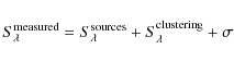
|
(A.1) |
where
If two populations of sources have very similar fluxes at the
wavelength of detection (24 ![]() m) and are situated at similar
redshifts, we can assume that their sources have very
similar physical characteristics and hence their colors
m) and are situated at similar
redshifts, we can assume that their sources have very
similar physical characteristics and hence their colors
![]() are very similar. In this case, we can write:
are very similar. In this case, we can write:
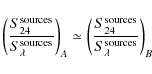
|
(A.2) |
where the A and B subscripts represent the first and second population of sources. We can measure the total flux (from the sources and the clustering) for the stacking of both source populations and express them as:
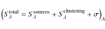
|
(A.3) |
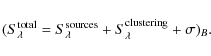
|
(A.4) |
If we were to assume that the contribution of the correlated sources to the flux is the same for both populations
The main problem for the applicability of this method is that we
need
to stack many sources to ensure that the noise becomes negligible
compared to
the signal. Because of this, it is preferable to combine an observation
whose photometry is affected by the clustering with another observation
for which this problem does not
exist, as illustrated by our present analysis. If the photometry of
this second observation is affected by
smaller errors (as it is the case of SCUBA-2 data relative to Planck
data at 850 ![]() m),
the results will be improved by combining the two
observations. However, the method discussed in this appendix is
applicable to cases where we do not have an alternative observation
with which we can correct from the clustering problem.
m),
the results will be improved by combining the two
observations. However, the method discussed in this appendix is
applicable to cases where we do not have an alternative observation
with which we can correct from the clustering problem.
References
- Amblard, A., & Cooray, A. 2007, ApJ, 670, 903 [NASA ADS] [CrossRef] [Google Scholar]
- Baldry, I., Liske, J., & Driver, S. P. 2008, GAMA: a new galaxy survey, in IAU Symp. 245, ed. M. Bureau, E. Athanassoula, & B. Barbuy, 83 [Google Scholar]
- Beelen, A., Omont, A., Bavouzet, N., et al. 2008, A&A, 485, 645 [NASA ADS] [CrossRef] [EDP Sciences] [Google Scholar]
- Bertoldi, F., Menten, K. M., Kreysa, E., Carilli, C. L., & Owen, F. 2000 [arXiv:astro-ph/0010553] [Google Scholar]
- Blain, A. W., Smail, I., Ivison, R. J., Kneib, J.-P., & Frayer, D. T. 2002, Phys. Rep., 369, 111 [NASA ADS] [CrossRef] [Google Scholar]
- Blain, A. W., Chapman, S. C., Smail, I., et al. 2004, ApJ, 611, 725 [NASA ADS] [CrossRef] [Google Scholar]
- Caputi, K. I., Dole, H., Lagache, G., et al. 2006, ApJ, 637, 727 [NASA ADS] [CrossRef] [Google Scholar]
- Delabrouille, J., Cardoso, J.-F., & Patanchon, G. 2003, MNRAS, 346, 1089 [NASA ADS] [CrossRef] [Google Scholar]
- Devlin, M. J., Ade, P. A. R., Aretxaga, I. 2009, Nature, 458, 737 [NASA ADS] [CrossRef] [PubMed] [Google Scholar]
- Dole, H., Gispert, R., & Lagache, G. 2001, A&A, 372, 364 [NASA ADS] [CrossRef] [EDP Sciences] [Google Scholar]
- Dole, H., Le Floc'h, E., Pérez-González, P. G., et al. 2004, ApJS, 154, 87 [NASA ADS] [CrossRef] [Google Scholar]
- Dole, H., Lagache, G., Puget, J.-L., et al. 2006, A&A, 451, 417 [NASA ADS] [CrossRef] [EDP Sciences] [MathSciNet] [Google Scholar]
- Dye, S., Eales, S. A., Ashby, M. L. N., et al. 2006, ApJ, 644, 769 [NASA ADS] [CrossRef] [Google Scholar]
- Elbaz, D. 2005, Space Sci. Rev., 119, 93 [NASA ADS] [CrossRef] [Google Scholar]
- Elbaz, D., Cesarsky, C. J., Chanial, P., et al. 2002, A&A, 384, 848 [NASA ADS] [CrossRef] [EDP Sciences] [Google Scholar]
- Farrah, D., Lonsdale, C. J., Borys, C., et al. 2006, ApJ, 641, L17 [NASA ADS] [CrossRef] [Google Scholar]
- Fernandez-Conde, N., Lagache, G., Puget, J.-L., et al. 2008, A&A, 481, 885 [NASA ADS] [CrossRef] [EDP Sciences] [Google Scholar]
- Fixsen, D. J., Dwek, E., Mather, J. C., Bennett, C. L., & Shafer, R. A. 1998, ApJ, 508, 123 [NASA ADS] [CrossRef] [Google Scholar]
- Genzel, R., & Cesarsky, C. J. 2000, ARA&A, 38, 761 [NASA ADS] [CrossRef] [Google Scholar]
- Haiman, Z., & Knox, L. 2000, ApJ, 530, 124 [NASA ADS] [CrossRef] [Google Scholar]
- Hauser, M. G., Arendt, R. G., Kelsall, T., et al. 1998, ApJ, 508, 25 [NASA ADS] [CrossRef] [Google Scholar]
- Ilbert, O., Capak, P., Salvato, M., et al. 2009, ApJ, 690, 1236 [NASA ADS] [CrossRef] [Google Scholar]
- Knox, L., Cooray, A., Eisenstein, D., et al. 2001, ApJ, 550, 7 [NASA ADS] [CrossRef] [Google Scholar]
- Lagache, G., Dole, H., & Puget, J.-L. 2003, MNRAS, 338, 555 [NASA ADS] [CrossRef] [Google Scholar]
- Lagache, G., Dole, H., Puget, J.-L., et al. 2004, ApJS, 154, 112 [NASA ADS] [CrossRef] [Google Scholar]
- Lagache, G., Puget, J.-L., & Dole, H. 2005, ARA&A, 43, 727 [NASA ADS] [CrossRef] [Google Scholar]
- Lagache, G., Bavouzet, N., & Fernandez-Conde, N. 2007, ApJ, 665, L89 [NASA ADS] [CrossRef] [Google Scholar]
- Lonsdale, C., Polletta, M. D. C., Surace, J., et al. 2004, ApJS, 154, 54 [NASA ADS] [CrossRef] [Google Scholar]
- Magliocchetti, M., Cirasuolo, M., McLure, R. J. 2008, MNRAS, 383, 1131 [NASA ADS] [CrossRef] [Google Scholar]
- Mainzer, A. K., Eisenhardt, P., Wright, E. L., Preliminary design of the Wide-Field Infrared Survey Explorer (WISE), in MacEwen, H. A, editor, UV/Optical/IR Space Telescopes: Innovative Technologies and Concepts II, ed. MacEwen, Howard A. Proc. SPIE of Presented at the Society of Photo-Optical Instrumentation Engineers, SPIE Conf., 5899, 262, [Google Scholar]
- Marsden, G., Ade, P. A. R., Bock, J. J., et al. 2009, ApJ, 707, 1729 [NASA ADS] [CrossRef] [Google Scholar]
- Papovich, C., Dole, H., Egami, E., et al. 2004, ApJS, 154, 70 [NASA ADS] [CrossRef] [Google Scholar]
- Puget, J.-L., Abergel, A., Bernard, J.-P., et al. 1996, A&A, 308, L5 [NASA ADS] [Google Scholar]
- Sanders, D. B., Salvato, M., Aussel, H., et al. 2007, ApJS, 172, 86 [Google Scholar]
- Serjeant, S., Dye, S., Mortier, A., et al. 2008, MNRAS, 386, 1907 [NASA ADS] [CrossRef] [Google Scholar]
- Viero, M. P., Ade, P. A. R., & Bock, J. J. 2009, ApJ, 707, 1766 [NASA ADS] [CrossRef] [Google Scholar]
- Wang, W.-H., Cowie, L. L., & Barger, A. J. 2006, ApJ, 647, 74 [NASA ADS] [CrossRef] [Google Scholar]
- Zheng, X. Z., Dole, H., & Bell, E. F. 2007, ApJ, 670, 301 [NASA ADS] [CrossRef] [Google Scholar]
Footnotes
- ... SWIRE
- http://ssc.spitzer.caltech.edu/legacy/
- ... (DES
- http://www.darkenergysurvey.org/
- ...Fernandez-Conde et al.
(2008)
- The simulations are publicly available at http://www.ias.u-psud.fr/irgalaxies
- ... (Big-)BOSS
- http://www.sdss3.org/cosmology.php
- ...
DES
- http://www.darkenergysurvey.org/
- ... work
- We analyze the stacking up to
 since
reliable estimates of the redshift up to that
redshift are available (although over quite
small areas).
since
reliable estimates of the redshift up to that
redshift are available (although over quite
small areas).
- ...m)
- To decrease the computation time, we increase the number of sources to be stacked using a logarithmic step of dN/N= 1.5.
- ... clustering)
- The problems associated with errors in the measurement of S24 are considered negligible (see Sanders et al. 2007).
- ... area
- And therefore should have
 times more signal-to-noise
ratio for similar populations of sources.
times more signal-to-noise
ratio for similar populations of sources.
- ... errors
- Note that the top right area with no data plotted
corresponds to a region where they are no sources at
24 microns; note also that in color representations as in
Fig. 5,
small differences in estimated value can have a great visual impact due
to the variation in colors. A mere 20% change in the estimate can
change the color from green to red. The general variation is consistent
with our detection threshold of 3
 .
.
- ... error
- Note that the mean flux relative error is equivalent to the mean color relative error since there is no error in our S24 measurements.
- ... webpage
- http://www.jach.hawaii.edu/JCMT/surveys/Cosmology.html
All Figures
|
|
Figure 1:
Top: input fluxes of the sources in the redshift slice 1.5<z<1.6
(solid line) together with estimates of the fluxes of the sources using
the smoothing technique (dashed line) and estimates of the fluxes of
the sources without smoothing (diamond). Bottom: the same but zoomed for
|
| Open with DEXTER | |
| In the text | |
|
|
Figure 2:
Histogram of the fluxes at 350 |
| Open with DEXTER | |
| In the text | |
|
|
Figure 3:
Histograms of the number of cold (thin line) and starburst (thick line) sources per 24 |
| Open with DEXTER | |
| In the text | |
|
|
Figure 4:
Ratio of recovered fluxes from stacking (
|
| Open with DEXTER | |
| In the text | |
|
|
Figure 5:
Accuracy in the mean recovered fluxes at 350 |
| Open with DEXTER | |
| In the text | |
|
|
Figure 6:
Relative errors in recovered fluxes for individual sources at 350 |
| Open with DEXTER | |
| In the text | |
|
|
Figure 7:
Same as Fig. 6 but for an
observation at 350 |
| Open with DEXTER | |
| In the text | |
|
|
Figure 8:
Left: real fluxes of the sources at 350 |
| Open with DEXTER | |
| In the text | |
|
|
Figure 9: Left: real S350/S24 flux ratio of the sources in the space S24-z. Right: S350/S24 flux ratio found by the smoothed stacking technique ( right). The colors correspond to different values of the ratio, while the vertical axis is S24 and the horizontal axis is the redshift bin. The S24-z space is divided linearly in z and logarithmically in S24. |
| Open with DEXTER | |
| In the text | |
|
|
Figure 10: Same as Fig. 5 but with no redshift errors. |
| Open with DEXTER | |
| In the text | |
|
|
Figure 11:
Lateral cut of a stacking image (Planck/HFI at 850 |
| Open with DEXTER | |
| In the text | |
|
|
Figure 12:
Relative errors in recovered fluxes for individual sources at 850 |
| Open with DEXTER | |
| In the text | |
|
|
Figure 13:
Accuracy of the mean recovered fluxes at 850 |
| Open with DEXTER | |
| In the text | |
| |
Figure 14:
Ratio of recovered to input fluxes of individual sources at 850 |
| Open with DEXTER | |
| In the text | |
|
|
Figure 15:
Relative error in the mean recovered fluxes at 850 |
| Open with DEXTER | |
| In the text | |
|
|
Figure 16:
Combined observations at 350 |
| Open with DEXTER | |
| In the text | |
|
|
Figure 17:
Same as Fig. 16 for combined observations at 850 |
| Open with DEXTER | |
| In the text | |
| |
Figure 18:
True mean fluxes (diamonds) compared to the mean
fluxes found by stacking (triangles) with the estimated errors at
70, 160, 250, 350, 500, and 850 |
| Open with DEXTER | |
| In the text | |
|
|
Figure 19: Power spectra of two
maps in which we placed the sources with either their input fluxes from
the simulations (dotted line) or their stacked fluxes (dashed line).
The results are shown for a SWIRE observation ( left figures) and COSMOS observation ( right figures) at 350 |
| Open with DEXTER | |
| In the text | |
|
|
Figure 20:
Same as Fig. 19 at 850 |
| Open with DEXTER | |
| In the text | |
|
|
Figure 21:
Power spectra of the map for a SWIRE observation at 350 |
| Open with DEXTER | |
| In the text | |
|
|
Figure 22: Same as Fig. 21 but for the COSMOS field. |
| Open with DEXTER | |
| In the text | |
|
|
Figure 23:
Power spectra of the 850 |
| Open with DEXTER | |
| In the text | |
|
|
Figure 24: Same as Fig. 23 but for the COSMOS field. |
| Open with DEXTER | |
| In the text | |
Copyright ESO 2010
Current usage metrics show cumulative count of Article Views (full-text article views including HTML views, PDF and ePub downloads, according to the available data) and Abstracts Views on Vision4Press platform.
Data correspond to usage on the plateform after 2015. The current usage metrics is available 48-96 hours after online publication and is updated daily on week days.
Initial download of the metrics may take a while.