| Issue |
A&A
Volume 515, June 2010
|
|
|---|---|---|
| Article Number | A86 | |
| Number of page(s) | 10 | |
| Section | Stellar structure and evolution | |
| DOI | https://doi.org/10.1051/0004-6361/200911835 | |
| Published online | 11 June 2010 | |
Absolute emission altitude of pulsars: PSRs B1839+09, B1916+14, and B2111+46
R. M. C. Thomas1 - R. T. Gangadhara2
1 - National Center for Radio Astrophysics, Pune - 411007, India
2 -
Indian Institute of Astrophysics, Bangalore - 560034, India
Received 12 February 2009 / Accepted 12 February 2010
Abstract
Aims. We study the mean profiles of the multi-component
pulsars PSRs B1839+09, B1916+14 and B2111+46. We estimate the
emission height of the core components, and hence find the absolute
emission altitudes corresponding to the conal components.
Methods. By fitting Gaussians to the emission components, we
determine the phase location of the component peaks. Our findings
indicate that the emission beams of these pulsars have the nested
core-cone structures. Based on the phase location of the component
peaks, we estimate the aberration-retardation (A/R) phase shifts in the
profiles. Due to the A/R phase shift, the peak of the core component in
the intensity profile and the inflection point of the polarization
angle swing are found to be symmetrically shifted in the opposite
directions with respect to the meridional plane in such a way that the
core shifts towards the leading side and the polarization angle
inflection point towards the trailing side.
Results. We have been able to locate the phase location of the
meridional plane and to estimate the absolute emission altitude of both
the core and the conal components relative to the neutron star center,
using the exact expression for the A/R phase shift given by Gangadhara
(2005).
Key words: stars: rotation - pulsars: individual: PSR B1839+09 - pulsars: individual: PSR B1916+14 - pulsars: individual: PSR B2111+46
1 Introduction
Pulsar radio emission is understood to be emitted by the relativistic plasma accelerated along the dipolar magnetic field lines (e.g., Ruderman & Sutherland 1975). Among the various models proposed for pulsar emission, the coherent curvature radiation has turned out to be an effective mechanism for explaining some of the important pulsar radiation properties. The common occurrence of an odd number of components in the mean pulsar profiles has lead to the nomenclature of a nested conal structure for the pulsar emission beam (e.g., Rankin 1983a; Rankin 1993). However, Lyne & Manchester (1988) suggested that the emission within the beam is patchy, i.e., the distribution of component locations within the beam is random rather than organized in one or more hollow cones. Also studies by Mitra & Deshpande (1999) indicate that the structure of the pulsar emission beam is more likely to be nested hollow cones. Gangadhara & Gupta (2001, hereafter GG01), and Gupta & Gangadhara (2003, hereafter GG03) showed that the prevalent picture of emission cones axially located around the central core component is a suitable model for explaining the core-cone structure of the pulsar emission beam.
A long-standing question in pulsar astronomy has been the location of the radio emission region in the magnetosphere. In the literature, there are mainly two types of methods proposed for estimating the radio emission altitudes: (1) a purely geometric method, which assumes the pulse edge is emitted from the last open field lines (e.g., Cordes 1978; Gil & Kijak 1993; Kijak & Gil 2003); (2) a relativistic phase shift method, which assumes that the asymmetry in the conal components phase location relative to the core is due to the aberration-retardation phase shift (e.g., GG01, Gangadhara 2005, hereafter G05). Both methods have merits and demerits: the first method has an ambiguity in identifying the last open field lines, while the latter is restricted to the profiles in which the core-cone structure can be clearly identified. The emission heights of PSR B0329+54 given in GG01, six other pulsars in GG03 and the revised ones by Dyks et al. (2004, hereafter DRH04) are all relative to the emission height of the core, which is assumed to be zero. However, the core emission is believed to originate from lower altitudes than that of the conal components (e.g., Blaskiewicz et al. 1991; Rankin 1993). Hoensbroech & Xilouris (1997) estimated the emission heights at high frequency radio profiles for a set of pulsars. They suggested that the emission heights at high frequency can set an upper limit for the core emission height.
By assuming a fixed emission altitude across the pulse, Blaskiewicz et al. (1991, hereafter BCW91) presented a relativistic rotating vector model. The results of this purely geometric method are found to be in rough agreement with those of BCW91. However, the relativistic phase shift method clearly indicates that the emission altitude across the pulse window is not constant (GG01; GG03; DRH04; Johnston & Weisberg 2006; Krzeszowski et al. 2009).
By considering the relativistically beamed radio emission in the direction of the magnetic field line tangents, Gangadhara (2004, hereafter G04) solved the viewing geometry in an inclined and slowly rotating dipole magnetic field. A more exact expression for the relativistic phase shift is given in (G05), which also includes the phase shift due to polar cap currents. In the present work, we analyze the mean profiles of PSRs B1839+09 and B1916+14 at 1418 MHz, and PSR B2111+46 at 610 MHz and 1408 MHz, to estimate the absolute emission height of the pulse components. In Sect. 2, we give a method for estimating the absolute emission height of pulse components.
2 Method for estimating the absolute emission heights
The work of BCW91 generalized the rotating vector model (RVM) to
include the relativistic effects due to rotation. According to their
model, the centroid of the intensity profile advances to an earlier
phase by ![]()
![]() while the polarization position angle
inflection point (PPAIP) is delayed to a later phase by
while the polarization position angle
inflection point (PPAIP) is delayed to a later phase by ![]()
![]() where r is the radial distance from the center of
neutron star and
where r is the radial distance from the center of
neutron star and
![]() is the light cylinder radius. After
estimating the width of the pulse at
is the light cylinder radius. After
estimating the width of the pulse at ![]()
![]() intensity level
and by fitting the relativistic rotating vector model, they estimated
the phase shift between the centroid of the profile and the PPAIP. But
the retardation phase shift was ignored in BCW91, as they assumed a
constant emission height across the pulse. In GG01, GG03, Johnston &
Weisberg (2006) and Krzeszowski et al. (2009) it was shown though that
the emission altitude is not constant across the pulse, and hence
retardation has to be taken into account while estimating the A/R
phase shifts. Further, Dyks et al. (2004) showed that the centroid of
the intensity profile advances by
intensity level
and by fitting the relativistic rotating vector model, they estimated
the phase shift between the centroid of the profile and the PPAIP. But
the retardation phase shift was ignored in BCW91, as they assumed a
constant emission height across the pulse. In GG01, GG03, Johnston &
Weisberg (2006) and Krzeszowski et al. (2009) it was shown though that
the emission altitude is not constant across the pulse, and hence
retardation has to be taken into account while estimating the A/R
phase shifts. Further, Dyks et al. (2004) showed that the centroid of
the intensity profile advances by ![]()
![]() while the
PPAIP is delayed by
while the
PPAIP is delayed by ![]()
![]() due to A/R effects with
respect to the meridional plane.
due to A/R effects with
respect to the meridional plane.
![\begin{figure}
\par\includegraphics[width=8cm,clip]{11835fg1.eps}
\end{figure}](/articles/aa/full_html/2010/07/aa11835-09/img11.png)
|
Figure 1: Schematic diagram showing the A/R phase shift between the core peak (CP) and the polarization position angle inflection point (PPAIP). The panel a) for the co-rotating frame, where the phases of PPAIP and CP coincide with that of the meridional plane (M), and b) in laboratory frame, due to A/R effects, both the PPAIP and the CP are symmetrically shifted in the opposite directions with respect to M. |
| Open with DEXTER | |
By solving the viewing geometry in the dipole magnetic field,
Gangadhara (2005) showed that instead of a centroid of intensity
profile, the phase shift of the central (core) peak (CP) relative to
the meridional plane must be considered for estimating the A/R phase
shifts. In the co-rotating (non-rotating) case both core and PPAIP
originate from the same phase (meridional plane M, see
Fig. 1a). Whereas in the observer (laboratory) frame, the CP shifts to
the earlier phase and the PPAIP to the later phase by the same
magnitude (see Fig. 1b). Hence to find the absolute emission height
of the profile components including the central (core) component, we
adapted the method of G05 to consider the CP instead of the
centroid of pulse (BCW91) for estimating the A/R phase shift. It
is logical to presume that the aforesaid r should be the same for
the origin of the central (core) component and the PPAIP. Or stated
otherwise, the phase difference
![]() in the co-rotating frame, where
in the co-rotating frame, where
![]() is the phase location of the core peak while
is the phase location of the core peak while
![]() is the phase location of the PPAIP.
is the phase location of the PPAIP.
As illustrated in Fig. 2, the panel (a) depicts the cross section of
the emission region in the co-rotating frame, while panel (b) shows for the
same in the observer's frame. The thick arrow represents the
direction of the rotation, and the thinner line the sweep of the
line-of-sight. The shaded ring-like region represents the nested conal
emission regions and the central circle the core emission region. The
sweep of the line-of-sight across the depicted region causes the core
peak and the PPAIP to be separated by a roughly equal measure (![]()
![]() )
in opposite directions from the meridional plane (M),
as illustrated in Fig. 1. The resultant intensity profile,
which characterizes a sum total of emissions after the line-of-sight
sweeps across the emission region, is shown in the adjoining box on the
right hand side.
)
in opposite directions from the meridional plane (M),
as illustrated in Fig. 1. The resultant intensity profile,
which characterizes a sum total of emissions after the line-of-sight
sweeps across the emission region, is shown in the adjoining box on the
right hand side.
| Figure 2: Schematic diagram to show the probable distribution of emission patterns across the pulsar beam. The beam cross sections as they appear in a) the co-rotating frame and b) the laboratory frame, where the cones are not coaxial with the central core because of A/R retardation effects. The thick horizontal line represents the direction of the tracing of the line-of-sight across the beam. The resultant intensity profile is shown in the adjoining box. The vertical line denotes the meridional plane, and the thick arrow represents the direction of the pulsar rotation. |
|
| Open with DEXTER | |
![\begin{figure}
\par\includegraphics[width=9cm,clip]{11835fg3.eps} \vspace*{-2mm}
\end{figure}](/articles/aa/full_html/2010/07/aa11835-09/img17.png)
|
Figure 3:
Intensity profile of PSR B1839+09 at
1418 MHz, fitted with the Gaussians to the sub-pulse
components. In panel a) the continuous line represents the observed
mean profile while the broken line curves represent the fitted
Gaussians. The arrow points to the phase of the core peak. In panel
b) the corresponding polarization angle ( |
| Open with DEXTER | |
![\begin{figure}
\par\includegraphics[width=9cm,clip]{11835fg4.eps} \vspace*{-2mm}
\end{figure}](/articles/aa/full_html/2010/07/aa11835-09/img18.png)
|
Figure 4: Intensity profile of PSR B1916+14 at 1418 MHz. See the caption of Fig. 3 for details. |
| Open with DEXTER | |
3 Application of the method
The implementation of the aforesaid method to estimate the absolute emission height of the core and conal components is described below. We considered the mean profiles of PSRs B1839+09, B1916+14 and B2111+46 for our study, as they exhibit a clearly identifiable core and smooth polarization-position-angle (PPA) swing. We obtained the data of PSRs B1839+09 and B1916+14 from Everette & Weisberg (2001), and those of PSR B2111+46 from EPN data base.
3.1 Longitude of the core peak
We fitted Gaussians to the pulse components to resolve the individual
components based on the method developed by Kramer et al. (1994), and
the profiles are given in Figs. 3-6. Hence the peak-phase locations of the individual components are resolved. The broken line curves in panel (a) indicate
the fitted Gaussians. The phase location of the core peak
![]() is marked with an arrow and is tabulated in
Table 1. The PPA is plotted in panel (b), and the vertical
lines mark the fitted region of the curve. The panel (c) shows the
zoomed-out region of the PPA within the region of the fit. The arrow
points to the PPAIP in both panels (b) and (c).
is marked with an arrow and is tabulated in
Table 1. The PPA is plotted in panel (b), and the vertical
lines mark the fitted region of the curve. The panel (c) shows the
zoomed-out region of the PPA within the region of the fit. The arrow
points to the PPAIP in both panels (b) and (c).
The location of the central component (core) is expected to appear at M
for an observer in the co-rotating frame as explained in
Sect. 2 and illustrated in Fig. 1a. But for an observer
in the laboratory frame, the core emission will be advanced to an
earlier phase by
![]() and the corresponding PPAIP delayed to a later phase by
and the corresponding PPAIP delayed to a later phase by
![]() where
where
![]() is the emission height of the core. Then the A/R phase
shift of the core with respect to M is
is the emission height of the core. Then the A/R phase
shift of the core with respect to M is
![]() and the parameters related to core emission are given in
Table 1. The frequency
and the parameters related to core emission are given in
Table 1. The frequency ![]() of each data set is given in
Col. 2, and the phase shifts
of each data set is given in
Col. 2, and the phase shifts
![]() and
and
![]() in Cols. 3 and 4.
in Cols. 3 and 4.
![\begin{figure}
\par\includegraphics[width=9cm,clip]{11835fg5.eps}
\end{figure}](/articles/aa/full_html/2010/07/aa11835-09/img27.png)
|
Figure 5: Intensity profile of PSR B2111+46 at 610 MHz. See the caption of Fig. 3 for details. |
| Open with DEXTER | |
![\begin{figure}
\par\includegraphics[width=9cm,clip]{11835fg6.eps}
\end{figure}](/articles/aa/full_html/2010/07/aa11835-09/img28.png)
|
Figure 6: Intensity profile of PSR B2111+46 at 1408 MHz. See the caption of Fig. 3 for details. |
| Open with DEXTER | |
3.2 The relativistic RVM fit
We fitted the relativistic RVM (BCW91) to the region of the PPA data, which corresponds to the core emission, the region over which the core polarization is significantly higher than that over the adjacent conal regions. We could see from the profiles that the pulse phase range falling within the full-width-at-half-maximum (FWHM) of the central-fit-Gaussian can clearly bracket out the emissions that dominate the core. The core emission is found to be dominant within 10% intensity levels of the central Guassian of the 1418 MHz data of PSR B1916+14, and hence we included that region for fitting the BCW91 curve for that profile. Additional reasons for restricting the fit region are discussed in detail in later sections.
Table 1: Core emission geometry parameters of PSRs B1839+09, B1916+14 and B2111+46.
Table 2: Conal emission geometry parameters of PSRs B1839+09, B1916+14 and B2111+46.
3.2.1 Longitude of polarization position angle inflection point
We invoked the guess values for the emission height r and the phase
![]() to fit the BCW91 curve. The polarization angle
data, falling within the FWHM of the core, are fitted with a 6th
degree polynomial:
to fit the BCW91 curve. The polarization angle
data, falling within the FWHM of the core, are fitted with a 6th
degree polynomial:
![]() where
where
![]() are
the fit coefficients, and
are
the fit coefficients, and ![]() is the pulse phase in degrees. We
differentiated the fitted polynomial and found the maximum of
is the pulse phase in degrees. We
differentiated the fitted polynomial and found the maximum of
![]() that gives the guess value of
that gives the guess value of
![]() In the next step, the PPA data were fitted with the relativistic RVM
curve (BCW91) using the following expression
In the next step, the PPA data were fitted with the relativistic RVM
curve (BCW91) using the following expression
![\begin{displaymath}
\psi_{\rm BCW}=\psi_0+ \tan^{-1}\left[\frac{\sin\alpha ~ \s...
...ta}{\sin\beta+\sin\alpha\cos\zeta(1-\cos(\Omega
t))}\right],
\end{displaymath}](/articles/aa/full_html/2010/07/aa11835-09/img105.png)
where
The parameter ![]() is inserted in the above Eq. (1)
in order to offset the possible arbitrary and constant ``vertical
shift'' that the raw PPA data might have. This is due to the arbitrary
value of the projection of the rotation axis in the sky plane. Since
we are interested in finding r, which is expected to be relatively
constant in the region of fit, we assumed it to be independent of
is inserted in the above Eq. (1)
in order to offset the possible arbitrary and constant ``vertical
shift'' that the raw PPA data might have. This is due to the arbitrary
value of the projection of the rotation axis in the sky plane. Since
we are interested in finding r, which is expected to be relatively
constant in the region of fit, we assumed it to be independent of
![]() ,
and hence it is taken as a fitting
parameter. The vertical shift in the raw PPA data, in the first
step, was brought closer to zero by finding a trial value for the
PPAIP on the vertical axis (
,
and hence it is taken as a fitting
parameter. The vertical shift in the raw PPA data, in the first
step, was brought closer to zero by finding a trial value for the
PPAIP on the vertical axis (
![]() )
from the polynomial fit,
and thereafter the data were shifted vertically so that
)
from the polynomial fit,
and thereafter the data were shifted vertically so that
![]() where
where
![]() is the observed polarization angle. These PPA data were fitted with
Eq. (1) keeping r and
is the observed polarization angle. These PPA data were fitted with
Eq. (1) keeping r and ![]() as the free
parameters; hence allowing two degrees of freedom for the fit
function, i.e., allowing the fit function to ``adjust'' in both
the vertical (through the free parameter
as the free
parameters; hence allowing two degrees of freedom for the fit
function, i.e., allowing the fit function to ``adjust'' in both
the vertical (through the free parameter ![]() )
and horizontal
direction (through free parameter r) for a good fit. The fit
procedure was repeated consecutively a few times, with the values of
r and
)
and horizontal
direction (through free parameter r) for a good fit. The fit
procedure was repeated consecutively a few times, with the values of
r and ![]() from the preceding fit as guess values for the final
convergent and stable values. Thus
from the preceding fit as guess values for the final
convergent and stable values. Thus
![]() was found
from the fit, and the corresponding values are shown in
Table 1. The geometric angles
was found
from the fit, and the corresponding values are shown in
Table 1. The geometric angles ![]() and
and ![]() were
not invoked as fit parameters in Eq. (1) because we
used their predetermined (published) values in the BCW91 fit
function. We used the values of
were
not invoked as fit parameters in Eq. (1) because we
used their predetermined (published) values in the BCW91 fit
function. We used the values of ![]() and
and ![]() given by
Everette & Weisberg (2001) for PSRs B1839+09 and B1916+14, and for
PSR B2111+46 by Mitra & Li (2004, hereafter ML04).
given by
Everette & Weisberg (2001) for PSRs B1839+09 and B1916+14, and for
PSR B2111+46 by Mitra & Li (2004, hereafter ML04).
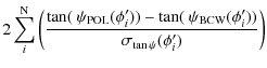
3.3 The longitude of the meridional plane
The CP and PPAIP of the polarization angle appear at M in the
co-rotating frame, as indicated by Fig. 1a. But they are
symmetrically shifted in opposite directions from M due to the A/R
phase shift for an observer in the laboratory frame, as indicated by
Fig. 1b. Note that the phase location of M is invariant
with respect to the rotation effects, or in other words, both the CP and
the PPAIP come closer to M at smaller r, and move away from it at
larger r. If
![]() and
and
![]() are the
estimated phases of the CP and the PPAIP, then their phase difference
(
are the
estimated phases of the CP and the PPAIP, then their phase difference
(
![]() )
is given by
)
is given by
![]() and the meridional plane M is situated at the mid point
between CP and PPAIP. Hence the phase of M is given by
and the meridional plane M is situated at the mid point
between CP and PPAIP. Hence the phase of M is given by
![]() In Figs. 3-6 the phases are shifted by
In Figs. 3-6 the phases are shifted by
![]() so that M appears at the zero phase and an arrow points to the phase location
so that M appears at the zero phase and an arrow points to the phase location
![]() in the polarization angle panels (b).
in the polarization angle panels (b).
3.4 The A/R phase shift of the core
The location of the central component (core) should appear at M for an
observer in the co-rotating frame as explained in
Sect. 2. But for an observer in the laboratory frame,
the core emission will be advanced to an earlier phase by
![]() and the
corresponding PPAIP be delayed to a later phase by
and the
corresponding PPAIP be delayed to a later phase by
![]() where
where
![]() is the
emission height of the core. Then the A/R phase shift of the core with
respect to M is
is the
emission height of the core. Then the A/R phase shift of the core with
respect to M is
![]()
3.5 Phase locations of the core and cone component peaks
We found the peak locations of the individual components by fitting
Gaussians to the mean profiles of the three pulsars. As mentioned in
Sect. 3.3, the data were shifted by
![]() so that M appears at zero phase. Because the A/R effects are absent
in the co-rotating frame, the conal components are expected to be
symmetrically located on either sides of meridional plane as
indicated by Fig. 2a. But in the laboratory frame, the
cones are advanced to an earlier phase due to the A/R effects and are
hence asymmetric with respect to the core location as indicated by
Fig. 2b. The meridional plane M is taken to be at the
zero phase, and the measured phases are, therefore, the absolute
phases with respect to M. Accordingly the estimated emission heights
are the absolute emission altitudes with respect to the center of the
neutron star.
so that M appears at zero phase. Because the A/R effects are absent
in the co-rotating frame, the conal components are expected to be
symmetrically located on either sides of meridional plane as
indicated by Fig. 2a. But in the laboratory frame, the
cones are advanced to an earlier phase due to the A/R effects and are
hence asymmetric with respect to the core location as indicated by
Fig. 2b. The meridional plane M is taken to be at the
zero phase, and the measured phases are, therefore, the absolute
phases with respect to M. Accordingly the estimated emission heights
are the absolute emission altitudes with respect to the center of the
neutron star.
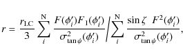
Let
![]() and
and
![]() be the peak locations of the
conal components on the leading and trailing sides of a pulse profile,
respectively. Then, using the following equations, we estimate the
A/R phase shift
be the peak locations of the
conal components on the leading and trailing sides of a pulse profile,
respectively. Then, using the following equations, we estimate the
A/R phase shift
![]() of the cone center with respect to M,
and the phase location
of the cone center with respect to M,
and the phase location ![]() of the component peaks in the
absence of the A/R phase shift, i.e., in the co-rotating frame (see
Eq. (11) in GG01):
of the component peaks in the
absence of the A/R phase shift, i.e., in the co-rotating frame (see
Eq. (11) in GG01):
4 The absolute emission heights
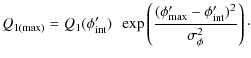
4.1 Emission height of the core
The core emission height was computed by using the
![]() in the expression for the A/R phase shift given by G05 (see
Eq. (45)). The parameters related to the core emission are given in
Table 1. In Col. 6 the emission heights are given as a
percentage of the light cylinder radius
in the expression for the A/R phase shift given by G05 (see
Eq. (45)). The parameters related to the core emission are given in
Table 1. In Col. 6 the emission heights are given as a
percentage of the light cylinder radius
![]() .
It shows that the
core emission in the radio band occurs over a range of altitude
spanning from 0.2 to 1 per cent of the light cylinder radius. The radio
frequency
.
It shows that the
core emission in the radio band occurs over a range of altitude
spanning from 0.2 to 1 per cent of the light cylinder radius. The radio
frequency ![]() of each data set is given in Col. 2, and the phase
shifts
of each data set is given in Col. 2, and the phase
shifts
![]() and
and
![]() in
Cols. 3 and 4, respectively. The values of
in
Cols. 3 and 4, respectively. The values of ![]() and the standard
residuals obtained are given in Cols. 7 and 8, respectively. The
foot location of magnetic field lines on the polar cap relative the
magnetic axis are given in Col. 9.
and the standard
residuals obtained are given in Cols. 7 and 8, respectively. The
foot location of magnetic field lines on the polar cap relative the
magnetic axis are given in Col. 9.
4.2 Emission height of the cones
We found the emission height of the cones based on the procedure that
is described in Sect. 3.5. In Col. 3 of
Table 2 we have given the cone numbers and the peak
locations of the conal components on the leading and trailing sides in
Cols. 4 and 5, respectively. The conal components are believed to
arise from the nested conal emissions (Rankin 1983a,b, 1990,
1993), which along with the central core emission make up the pulsar
emission beam. In Col. 6 of Table 2, we have given the
values of
![]() In general it increases in magnitude from the
innermost cone to the outer cone. The half-opening angle
In general it increases in magnitude from the
innermost cone to the outer cone. The half-opening angle ![]() (see Eq. (7) in G04) of the emission beam is given in Col. 7. Using
the exact formalism for the A/R phase shift (see Eq. (45) in G05), we
computed the emission heights and show them in Col. 8. Their percentage
values in
(see Eq. (7) in G04) of the emission beam is given in Col. 7. Using
the exact formalism for the A/R phase shift (see Eq. (45) in G05), we
computed the emission heights and show them in Col. 8. Their percentage
values in
![]() are given in Col. 9. In Col. 10, we
give the normalized co-latitude
are given in Col. 9. In Col. 10, we
give the normalized co-latitude
![]() of the foot field
lines on the polar cap, which are associated with the component
emissions. Due to the relativistic beaming and restrictions owing to
geometry, we find that the observer tends to receive the emissions
from open field lines, which are located in the foot locations ranging
from (approximately) 0.1 (Table 1) to 0.8 (Table 2) on the polar cap.
of the foot field
lines on the polar cap, which are associated with the component
emissions. Due to the relativistic beaming and restrictions owing to
geometry, we find that the observer tends to receive the emissions
from open field lines, which are located in the foot locations ranging
from (approximately) 0.1 (Table 1) to 0.8 (Table 2) on the polar cap.
4.3 PSR B1839+09
By fitting three Gaussians to the mean intensity profile of PSR
B1839+09 we have identified three sub-pulse components: a central
component and a pair of outer components flanking the central one. By
invoking the picture of a nested cone structure we infer that the outer
pair of components corresponds to a conal emission. The inner component
might be due to emissions close to the magnetic axis or because of the
``grazing-cut'' of the line-of-sight with an inner ring of emission. The
point of emission for the central component should fall in the
meridional plane M in the co-rotating frame of the pulsar in either of
the cases. We clearly identified the phase locations for the PPAIP
and the CP relative to the meridional plane M for PSR
B1839+09. The absolute emission heights estimated for the core and
conal component are given in Tables 1 and 2,
respectively. The emission heights of the central (core) component and
cone are found to be ![]() 50 km and
50 km and ![]() 60 km, respectively.
60 km, respectively.
4.4 PSR B1916+14
By fitting Gaussians to the intensity profile, we could identify three
sub-pulse components: a central component and a pair of outer
components flanking the central one. We clearly identified the
phase locations of the PPAIP and the central peak, and found the phase of
meridional plane M. The absolute emission heights, estimated for the
central (core) and conal components, are given in Tables 1
and 2. The emission heights of the central component and
the cone are estimated to be ![]() 100 km and
100 km and ![]() 300 km,
respectively.
300 km,
respectively.
4.5 PSR B2111+46
It is a well-studied pulsar. By fitting Gaussians to its intensity
profiles at frequencies 610 MHz and 1408 MHz, we could
identify five
sub-components: a central (core) component, a pair of inner components
and a pair of outer components. Our values of the phase locations of
the component peaks are in close agreement with the ones given by Zhang
et al. (2007) for PSR B2111+46. One can guess at the presence of
two inner components hidden between the core and the outer components
even by visual inspection. These two hidden components were detected in
the
previous work of GG03 in the 333 MHz single pulse data. The
absolute
emission heights estimated for the core and the cones are given in
Tables 1 and 2. The core emission height is
found to be ![]() 500 km at 610 MHz and
500 km at 610 MHz and ![]() 80 km at 1408 MHz. It
has been reported in ML04 that the widths of the core tend to show a
significant frequency evolution in their chosen set of six pulsars,
and hence they argued that the core emission does not come from the
stellar surface. However, we need to consider more high quality data
sets at different frequencies to see the frequency evolution of the core
emission height, and whether it follows any radius-to-frequency mapping.
80 km at 1408 MHz. It
has been reported in ML04 that the widths of the core tend to show a
significant frequency evolution in their chosen set of six pulsars,
and hence they argued that the core emission does not come from the
stellar surface. However, we need to consider more high quality data
sets at different frequencies to see the frequency evolution of the core
emission height, and whether it follows any radius-to-frequency mapping.
5 Results and discussions
Based on the A/R method, we estimated the absolute emission height of the core as well as cones in three pulsars: PSRs B1839+09, B1916+14 and B2111+46. Though this method is based on the existing standard models in literature, the combination of the A/R phase shift and the delay-radius relation of BCW91 for estimating the core height is novel.
The geometrical method, involving a comparison of the measured pulse
widths with geometrical predictions from dipolar models, is believed
to yield absolute emission heights. However, the estimation of
emission height, using the geometrical method, is based on the
assumption that the pulse edges originate from the last open field
lines of the polar cap. In general, the edge of the on-pulse region
may not originate from the last open field line, and hence the
assigning of the edges of the intensity profile to the last open field
lines can be misleading. For example, the range of magnetic
foot-colatitude for field-lines that are associated with components in
PSR B2111+46 are in the range from
![]() to 0.5,
whereas the last open field line is at 1. This means that the
boundary of the active region of emission can lie anywhere from
to 0.5,
whereas the last open field line is at 1. This means that the
boundary of the active region of emission can lie anywhere from ![]() 0.5 to 1.
0.5 to 1.
According to DRH04, the A/R phase shift advances the centroid of the
intensity profile to an earlier phase by
![]() while the PPAIP is delayed to a later phase by
while the PPAIP is delayed to a later phase by
![]() where
where
![]() is the emission height from the last open
field-line and
is the emission height from the last open
field-line and
![]() is the emission height of the core.
Then
is the emission height of the core.
Then
![]() and
the emission height
and
the emission height
![]() gives only an average of the emission height for
the core and the pulse edge, which is far from the true value. This
emission height cannot represent any specific pulse sub-component of
the profile, and can be misleading in cases where
gives only an average of the emission height for
the core and the pulse edge, which is far from the true value. This
emission height cannot represent any specific pulse sub-component of
the profile, and can be misleading in cases where
![]() and
and
![]() are significantly different. Further more, this will
introduce large systematic errors in the emission heights estimated
from geometrical methods, due to the aforesaid assumption of
identifying the last open field lines with the pulse edges.
are significantly different. Further more, this will
introduce large systematic errors in the emission heights estimated
from geometrical methods, due to the aforesaid assumption of
identifying the last open field lines with the pulse edges.
Rankin (1983a) has argued that the pulsar emission cones are
quasi-axial, i.e., the conal components are not exactly axially
located with respect to the magnetic axis. Mitra & Deshpande (1999)
have suggested that the pulsar emission beams are nearly circular in
the aligned configuration (
![]() )
and change to
elliptical in the orthogonal configuration
)
and change to
elliptical in the orthogonal configuration
![]() .
The majority of the pulsar observations indicate that the beam
geometry is likely to be nested cones, distributed in a nearly
non-coaxial fashion about the magnetic axis. A likely case is that
the cones, which are coaxial in the co-rotating frame, will appear
non-coaxial in the laboratory frame because of the A/R phase shifts
(GG01; GG03).
.
The majority of the pulsar observations indicate that the beam
geometry is likely to be nested cones, distributed in a nearly
non-coaxial fashion about the magnetic axis. A likely case is that
the cones, which are coaxial in the co-rotating frame, will appear
non-coaxial in the laboratory frame because of the A/R phase shifts
(GG01; GG03).
In the works GG01 and GG03, the emission height of the core was neglected by assuming that it is considerably smaller than that of the components. However, we find that the emission height of the core is quite significant and cannot be neglected in comparison to the emission height of the components. We identify the meridional plane M as being located at the mid point between the centroid of the intensity profile and the PPAIP, owing to the A/R effects. By recognizing this, we were able to estimate the absolute emission heights of both the core and the conal components.
As mentioned before, we restricted the region of the fit of the BCW91 (relativistic RVM) curve to the section of the PPA data falling within the FWHM of the core component for estimating the core emission height, and the justification for doing so is given now. The expression for the BCW91 was derived by assuming that the emission altitude across the active region of the pulse profile is a constant. Thus in a BCW91 fitting, a single r value was taken to characterize the emission height of the full region of the PPA data. But later observational results (e.g., GG01; GG03) established that the emission altitude corresponding to the subpulse components in multi-component profiles spans over a large range of emission heights. This elicits the fact that in multi-component profiles the r, found by fitting the BCW91 curve to the full PPA region of the active profile, might give an emission altitude that can be significantly different from those obtained from the A/R method for the subpulse components.
The best-fit value of r in the BCW91 model, which is the weighted average of ri that characterize the emission height at each point of pulse phase, is given by Eq. (C.8) in Appendix C. Hence a single value of r found from the BCW91 fit cannot be closer to the true emission height corresponding to the core or cone peak if ri varies significantly within the region of the fit. For example, one can compare the emission altitudes in our Tables 1 and 2 with those given in Table 3 of ML04 for PSR B2111+46. It can be surmised that a single value of rcannot characterize the emission altitude across the entire active region of a multi-component profile.
We can think of two viable alternatives in this scenario: either (1)
adapt or modify the BCW91 formulation for a variable
emission altitude r (Dyks 2008) or (2) fit the BCW91 curve for
regions of the PPA profile having a relatively constant value of r.We prefer the latter alternative to evade the modification of
the theory behind the BCW91 model. Here we note that ![]() and
and
![]() are not invoked as fit parameters; instead we used
their published values in Eq. (C.1). This is expected to
further reduce the ambiguity of the fit results and to aid in
counteracting an obvious disadvantage in this ``restricted'' fit method,
i.e., having a reduced number of fitted PPA data points than a fit for
the ``full range'' of PPA data. It is remarkable that some of the fit
statistics (e.g., reduced
are not invoked as fit parameters; instead we used
their published values in Eq. (C.1). This is expected to
further reduce the ambiguity of the fit results and to aid in
counteracting an obvious disadvantage in this ``restricted'' fit method,
i.e., having a reduced number of fitted PPA data points than a fit for
the ``full range'' of PPA data. It is remarkable that some of the fit
statistics (e.g., reduced ![]() )
given in Table 1
reveal that the present method of fitting is comparable (in a few
cases even better) to the existing ones in the literature (e.g.,
compare the
)
given in Table 1
reveal that the present method of fitting is comparable (in a few
cases even better) to the existing ones in the literature (e.g.,
compare the ![]() value given in Table 1 with Table 2
of ML04 for PSR B2111+46). We estimated the standardized
residuals (SR) and found the percentage of SR that falls within -2 and
+2 as given in Col. (8) of Table 1. As it is known, a
good fit is expected to have a threshold 95% of the standardized
residuals to fall within -2 and +2. Several previous works found
that
value given in Table 1 with Table 2
of ML04 for PSR B2111+46). We estimated the standardized
residuals (SR) and found the percentage of SR that falls within -2 and
+2 as given in Col. (8) of Table 1. As it is known, a
good fit is expected to have a threshold 95% of the standardized
residuals to fall within -2 and +2. Several previous works found
that ![]() and
and ![]() are highly covariant in PPA fits (e.g.,
Everette & Weisberg 2001). But this covariance of
are highly covariant in PPA fits (e.g.,
Everette & Weisberg 2001). But this covariance of ![]() and
and
![]() with the r parameter was not mentioned by any of them. The fit
statistics do not reveal any significant covariance of
with the r parameter was not mentioned by any of them. The fit
statistics do not reveal any significant covariance of ![]() and
and
![]() with r. This gives us a further clue for finding the rparameter without invoking a concurrent fit for
with r. This gives us a further clue for finding the rparameter without invoking a concurrent fit for ![]() and
and ![]() (see Appendix A for the fitting procedure).
(see Appendix A for the fitting procedure).
Owing to the extreme difficulties encountered in determining ![]() and
and ![]() through RVM fitting, a larger range of PPA data have
always been preferred for a better fit (e.g., Everette & Weisberg
2001). The justification for doing so is that
through RVM fitting, a larger range of PPA data have
always been preferred for a better fit (e.g., Everette & Weisberg
2001). The justification for doing so is that ![]() and
and ![]() must remain constant throughout the entire PPA profile. But in the
present scenario, as described earlier, the selection of a large range
of PPA data for fitting does not always translate into a better
estimation of r because of the variation of the emission height with
pulse phase. So, owing to all of the above said reasons we restrict
the fit of the BCW91 curve to the PPA profile, falling around the core
component, which is expected to yield an emission altitude
characterizing the core height.
must remain constant throughout the entire PPA profile. But in the
present scenario, as described earlier, the selection of a large range
of PPA data for fitting does not always translate into a better
estimation of r because of the variation of the emission height with
pulse phase. So, owing to all of the above said reasons we restrict
the fit of the BCW91 curve to the PPA profile, falling around the core
component, which is expected to yield an emission altitude
characterizing the core height.
A section of inner cones often lapses over the core as is seen in the Gaussian fits (panel (a) of Figs. 3-6) of the total intensity profiles. The inner cones may contribute to the core polarization near the edges of pulse phase of the FWHM region that we bracketed. Hence the PPA corresponding to the bracketed region will be ``contaminated'' by the adjacent conals, and this has to be accounted for. We estimated and accounted for the error induced because of this effect in the estimation of the core emission heights (see Appendices B and C).
The possibility that the A/R phase shift may be reduced by the
rotational distortion of the magnetic field line due to a sweep-back
of the vacuum dipole magnetic field lines has to be considered. The
sweep-back of dipole magnetic field lines was first treated in detail
by Shitov (1983). Further, Dyks & Harding (2004) investigated
the rotational distortion of pulsar magnetic field by making the
approximation of a vacuum magnetosphere. For
![]()
![]() and
and
![]() we computed the phase shift
we computed the phase shift
![]() due to the magnetic field sweep-back (Dyks &
Harding 2004; also see Eq. (49) in G05). It is found to be
<0.0001 rad for
due to the magnetic field sweep-back (Dyks &
Harding 2004; also see Eq. (49) in G05). It is found to be
<0.0001 rad for
![]() which is much smaller than
the aberration, retardation and polar cap current phase shifts in
PSR B2111+46. Hence we neglect the magnetic field sweep-back effect.
which is much smaller than
the aberration, retardation and polar cap current phase shifts in
PSR B2111+46. Hence we neglect the magnetic field sweep-back effect.
The field-aligned polar-cap current does not introduce any significant phase shift into the phase of the PPAIP. But it introduces a positive offset into the PPA, though it roughly cancels due to the negative offset by aberration (Hibschman & Arons 2001). The phase shift of pulse components due to the polar cap current was estimated recently by G05, and found to be quite small compared to the A/R phase shift.
6 Summary
We analyzed the mean profiles of PSRs B1839+09 and B1916+14 at 1418 MHz, and those of B2111+46 at 610 MHz and 1408 MHz. The phase of the peak of central component (core) and that of the polarization position angle inflection point are symmetrically shifted in the opposite directions with respect to the meridional plane due to A/R effects. By recognizing this, we were able to locate the phase of the meridional plane and to estimate the absolute emission altitudes of the core and the conal components relative to the center of the neutron star. We used the exact expression for the phase shift given recently by G05. In all the cases we found that the core emission occurs at a relatively lower altitudes than the conal emissions. It is also interesting to note that the core emission at different frequencies in PSR B2111+46 falls in a range of altitude of 80 km at 1408 MHz to about 500 km at 610 MHz. It is clear that the low frequency emission comes from a higher height than that at high frequency. However, to confirm whether the core emission heights also obey any radius-to-frequency mapping demands the recursive analysis with high quality multi-frequency data. We plan to employ the methods described in this paper for the study of a few other pulsars with high quality data.
AcknowledgementsWe thank Joel Weisberg for providing the data of PSRs B1839+09 and B1916+14 at 1418 MHz. We used the data available on EPN archive maintained by MPIfR, Bonn, and thank all the observers who have made their data available on the EPN data base. We thank Yashwant Gupta for the helpful comments.
Appendix A: Estimation of 1

We apply the standard methods of statistics for fitting the
observed data with the model. For fitting
the PPA data with the BCW91 curve we define the reduced ![]() as
as
![\begin{displaymath}
\chi^2= \sum_{i}^{\rm N} \left[\frac{\psi_{\rm POL}(\phi'_{...
...si_{\rm BCW}(\phi'_{i})}{\sigma_{\psi}(\phi'_{i})} \right]^2 ,
\end{displaymath}](/articles/aa/full_html/2010/07/aa11835-09/img139.png)
where
For profile regions with a very high value of
![]() i.e., for
i.e., for
![]() the
the
![]() is taken as
is taken as
|
(A.2) |
where
where
|
(A.4) |
We set up a table of the integration values of the integral against a series of discrete P0 values and the
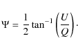
Appendix B: Polarization angle  :
contribution from the
adjacent component to the core
:
contribution from the
adjacent component to the core
The polarization angle ![]() is defined as
is defined as
Defining
where U1 and Q1 are taken as sufficiently small,

The expression for
| (B.9) |
provided U1 and Q1 are sufficiently small, so that
We use the above expressions for estimating the contribution to
![]() from the adjacent conal components. The suffix ``1'' indicates
the U and Q contribution solely from the inner cone, while the
suffix ``0'' indicates the pure core contribution for the same. We
employ approximations to find the value of U1 and Q1.
from the adjacent conal components. The suffix ``1'' indicates
the U and Q contribution solely from the inner cone, while the
suffix ``0'' indicates the pure core contribution for the same. We
employ approximations to find the value of U1 and Q1.
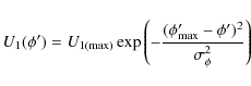
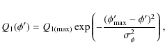
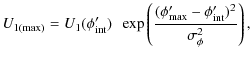
Since the total intensity of an inner conal component can be fitted
with a Gaussian, we make an assumption that the
![]() and
and
![]() also follow a Gaussian shape within the adjacent conal
component. Thus
also follow a Gaussian shape within the adjacent conal
component. Thus
and
where
Using Eqs. (B.12) and (B.13), we can find
Note: The PSR B1839+09 has practically no contribution of
polarization from the adjacent conals to the bracketed core
region. Hence this analysis is not performed for it. The
![]() and
and
![]() for PSR B1916+14 are the values at the
peak phases of the adjacent cones and are directly found from the
profile data. So, Eqs. (B.12) and (B.13) are not applicable for it. Hence the above-said analysis is done for the profiles of PSR B2111+46 only.
for PSR B1916+14 are the values at the
peak phases of the adjacent cones and are directly found from the
profile data. So, Eqs. (B.12) and (B.13) are not applicable for it. Hence the above-said analysis is done for the profiles of PSR B2111+46 only.
Appendix C: Determination of the r parameter: correcting for adjacent conal contribution
Here, we explain the scheme of the determination of r and
![]() using the BCW91 method with predetermined
values of
using the BCW91 method with predetermined
values of ![]() and
and ![]() .
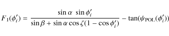
Consider the expression for the
polarization angle given in BCW91:
.
Consider the expression for the
polarization angle given in BCW91:
![\begin{displaymath}
\psi_{\rm BCW}(\phi_{i})= \tan^{-1}
\left[\frac{\sin\alph...
...a}{\sin\beta+\sin\alpha\cos\zeta(1-\cos\phi_{i})}\right]\cdot
\end{displaymath}](/articles/aa/full_html/2010/07/aa11835-09/img190.png)
Here define
![\begin{displaymath}
\chi^2= \sum_{i}^{\rm N} \left[\frac{\tan[~ \psi_{\rm POL}(...
...rm BCW}(\phi'_{i})]}{\sigma_{\tan\psi}(\phi'_{i})} \right]^2 ,
\end{displaymath}](/articles/aa/full_html/2010/07/aa11835-09/img191.png)
where
By minimizing the ![]() with respect to the parameter r, we can write
with respect to the parameter r, we can write
| |
= | 
|
|
By substituting for
where
|
(C.4) |
and
|
(C.5) |
If ri is a value so that
Then by substituting Eq. (C.6) into (C.3), we get
Within the bracketed region the small angle approximation for
or, by using
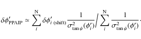
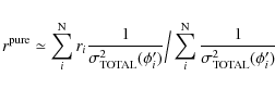
These expressions (C.8) and (C.9) show that the BCW fit of the PPA data is a weighted average of the emission heights ri of each data point. If some of the data points are corrupted by the adjacent conals, then the true linear polarization due to the core alone should be less than the observed. Hence it implies that the true PPA value corresponding to the pure core contribution should be slightly different from the observed PPA, which has a small mixture of contribution from adjacent conal component. An approximate method to estimate this error in the PPA (
![\begin{displaymath}\sigma_{\rm TOTAL}(\phi'_{i})
=\sqrt{\sigma_{\tan\psi}^2(\phi'_{i}) +\tan^2[\Delta\Psi_{\rm
cone}(\phi'_{i})]},
\end{displaymath}](/articles/aa/full_html/2010/07/aa11835-09/img210.png)
which takes into account the ``contamination'' of the core due to the adjacent cones. Thus we find
and
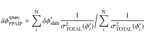
using the expressions (C.8) and (C.9). In principle,

where
In the actual fitting procedure we used the form of ![]() as
given in Appendix A. We estimated
as
given in Appendix A. We estimated
![]() for the profiles, and the values of
for the profiles, and the values of
![]() (Table 1) were attributed with an error factor as
given by Eq. (C.12). A set of weights are found in the
form of
(Table 1) were attributed with an error factor as
given by Eq. (C.12). A set of weights are found in the
form of
![]() The BCW91 model is fitted within the bracketed region
after (1) weighting the data with weights
The BCW91 model is fitted within the bracketed region
after (1) weighting the data with weights
![]() and (2) again
by weighting the data with weights
and (2) again
by weighting the data with weights
![]() The case
(1) will yield the phase shift for the PPAIP, while the case (2) should
yield the phase shift for the PPAIP with reduced weights to the PPA
points where the conal contributions are present. The difference in
the phase shifts found by case (1)and (2) should characterize the
extra increment (decrement) in core emission height due to the adjacent
conal contributions. The square of this phase shift difference is
added with the squared error of the PPAIP phase shift, and the square root
of this sum will give the improved error factor for the core emission
height. This improved error factor will take into account the
error induced in the estimation of the PPAIP in the bracketed region
due to the adjacent conal contribution.
The case
(1) will yield the phase shift for the PPAIP, while the case (2) should
yield the phase shift for the PPAIP with reduced weights to the PPA
points where the conal contributions are present. The difference in
the phase shifts found by case (1)and (2) should characterize the
extra increment (decrement) in core emission height due to the adjacent
conal contributions. The square of this phase shift difference is
added with the squared error of the PPAIP phase shift, and the square root
of this sum will give the improved error factor for the core emission
height. This improved error factor will take into account the
error induced in the estimation of the PPAIP in the bracketed region
due to the adjacent conal contribution.
References
- Blaskiewicz, M., Coders, J. M., & Wasserman, I. 1991, ApJ, 370, 643 (BCW91) [NASA ADS] [CrossRef] [Google Scholar]
- Cordes, J. M. 1978, ApJ, 222, 1006 [NASA ADS] [CrossRef] [PubMed] [Google Scholar]
- Dyks, J. 2008, MNRAS, 391, 859 [NASA ADS] [CrossRef] [Google Scholar]
- Dyks, J., & Harding, A. K. 2004, ApJ, 614, 869 [NASA ADS] [CrossRef] [Google Scholar]
- Dyks, J., Rudak, B., & Harding, A. K. 2004, ApJ, 607, 939 (DRH04) [NASA ADS] [CrossRef] [Google Scholar]
- Everette, J. E., & Weisberg, J. M. 2001, ApJ, 341, 357 [Google Scholar]
- Gangadhara, R. T. 2004, ApJ, 609, 335 (G04) [NASA ADS] [CrossRef] [Google Scholar]
- Gangadhara, R. T. 2005, ApJ, 628, 930 (G05) [Google Scholar]
- Gangadhara, R. T., & Gupta, Y. 2001, ApJ, 555, 31 (GG01) [NASA ADS] [CrossRef] [Google Scholar]
- Gil, J. A., & Kijak, J. 1993, A&A, 273, 563 [NASA ADS] [Google Scholar]
- Gupta, Y., & Gangadhara, R. T. 2003, ApJ, 584, 41 (GG03) [Google Scholar]
- Hibschman, J. A., & Arons, J. 2001, ApJ, 546, 382 [NASA ADS] [CrossRef] [Google Scholar]
- Hoensbroech, von A., & Xilouris, K. M. 1997, A&A, 324, 981 [NASA ADS] [Google Scholar]
- Johnston, S., & Weisberg, J. M. 2006, MNRAS, 368, 1856 [NASA ADS] [CrossRef] [Google Scholar]
- Kijak, J., & Gil, J. 2003, A&A, 397, 969 [NASA ADS] [CrossRef] [EDP Sciences] [Google Scholar]
- Kramer, M., Wielebinski, R., Jessner, A., Gil, J. A., & Seiradakis, J. H. 1994, A&AS, 107, 515 [NASA ADS] [Google Scholar]
- Krzeszowski, K., Mitca, D., Gupta, Y., et al. 2009, MNRAS, 393, 1617 [NASA ADS] [CrossRef] [Google Scholar]
- Lyne, A. G., & Manchester, R. N. 1988, MNRAS, 234, 477 [NASA ADS] [CrossRef] [Google Scholar]
- Mitra, D., & Deshpande, A. A. 1999, A&A, 346, 906 [NASA ADS] [Google Scholar]
- Mitra, D., & Li, X. H. 2004, A&A, 421, 215 (ML04) [NASA ADS] [CrossRef] [EDP Sciences] [Google Scholar]
- Naghizadeh-Khouei, J., & Clarke, D. 1993, A&A, 274, 968 [NASA ADS] [Google Scholar]
- Rankin, J. M. 1983a, ApJ, 274, 333 [NASA ADS] [CrossRef] [Google Scholar]
- Rankin, J. M. 1983b, ApJ, 274, 359 [Google Scholar]
- Rankin, J. M. 1990, ApJ, 352, 247 [NASA ADS] [CrossRef] [Google Scholar]
- Rankin, J. M. 1993, ApJS, 85, 145 [NASA ADS] [CrossRef] [Google Scholar]
- Ruderman, M. A., & Sutherland, P. G. 1975, ApJ, 196, 51 [NASA ADS] [CrossRef] [EDP Sciences] [Google Scholar]
- Shitov, Yu. P. 1983, SVA, 27, 314 [Google Scholar]
- Zhang, H., Qiao, G. J., Han, J. L., Lee, K. J., & Wang, H. G. 2007, A&A, 465, 525 [NASA ADS] [CrossRef] [EDP Sciences] [Google Scholar]
All Tables
Table 1: Core emission geometry parameters of PSRs B1839+09, B1916+14 and B2111+46.
Table 2: Conal emission geometry parameters of PSRs B1839+09, B1916+14 and B2111+46.
All Figures
|
|
Figure 1: Schematic diagram showing the A/R phase shift between the core peak (CP) and the polarization position angle inflection point (PPAIP). The panel a) for the co-rotating frame, where the phases of PPAIP and CP coincide with that of the meridional plane (M), and b) in laboratory frame, due to A/R effects, both the PPAIP and the CP are symmetrically shifted in the opposite directions with respect to M. |
| Open with DEXTER | |
| In the text | |
| |
Figure 2: Schematic diagram to show the probable distribution of emission patterns across the pulsar beam. The beam cross sections as they appear in a) the co-rotating frame and b) the laboratory frame, where the cones are not coaxial with the central core because of A/R retardation effects. The thick horizontal line represents the direction of the tracing of the line-of-sight across the beam. The resultant intensity profile is shown in the adjoining box. The vertical line denotes the meridional plane, and the thick arrow represents the direction of the pulsar rotation. |
| Open with DEXTER | |
| In the text | |
|
|
Figure 3:
Intensity profile of PSR B1839+09 at
1418 MHz, fitted with the Gaussians to the sub-pulse
components. In panel a) the continuous line represents the observed
mean profile while the broken line curves represent the fitted
Gaussians. The arrow points to the phase of the core peak. In panel
b) the corresponding polarization angle ( |
| Open with DEXTER | |
| In the text | |
|
|
Figure 4: Intensity profile of PSR B1916+14 at 1418 MHz. See the caption of Fig. 3 for details. |
| Open with DEXTER | |
| In the text | |
|
|
Figure 5: Intensity profile of PSR B2111+46 at 610 MHz. See the caption of Fig. 3 for details. |
| Open with DEXTER | |
| In the text | |
|
|
Figure 6: Intensity profile of PSR B2111+46 at 1408 MHz. See the caption of Fig. 3 for details. |
| Open with DEXTER | |
| In the text | |
Copyright ESO 2010
Current usage metrics show cumulative count of Article Views (full-text article views including HTML views, PDF and ePub downloads, according to the available data) and Abstracts Views on Vision4Press platform.
Data correspond to usage on the plateform after 2015. The current usage metrics is available 48-96 hours after online publication and is updated daily on week days.
Initial download of the metrics may take a while.