| Issue |
A&A
Volume 514, May 2010
|
|
|---|---|---|
| Article Number | A78 | |
| Number of page(s) | 6 | |
| Section | Interstellar and circumstellar matter | |
| DOI | https://doi.org/10.1051/0004-6361/200913959 | |
| Published online | 26 May 2010 | |
Studying the small scale ISM structure with supernovae
F. Patat1 - N. L. J. Cox2,3 - J. Parrent4,5 - D. Branch4
1 - European Organization for Astronomical Research in the Southern
Hemisphere (ESO), K. Schwarzschild-str. 2, 85748 Garching b.
München, Germany
2 - Herschel Science Centre, European Space Astronomy Centre, ESA, PO
Box 78, 28691 Madrid, Spain
3 - Institute of Astronomy, K.U. Leuven, Celestijnenlaan 200D, 3001
Leuven, Belgium
4 - Department of Physics and Astronomy. University of Oklahoma,
Norman, OK 73019, USA
5 - Department of Physics and Astronomy, Dartmouth College, Hanover, NH
03755-3528, Germany
Received 23 December 2009 / Accepted 25 February 2010
Abstract
Aims. In this work we explore the possibility of
using the fast expansion of a type Ia supernova photosphere to
detect extra-galactic ISM column density variations on spatial scales
of ![]() 100 AU
on time scales of a few months.
100 AU
on time scales of a few months.
Methods. We constructed a simple model which
describes the expansion of the photodisk and the effects of a patchy
interstellar cloud on the observed equivalent width of Na I
D lines. Using this model we derived the behavior of the equivalent
width as a function of time, spatial scale and amplitude of the column
density fluctuations.
Results. The calculations show that isolated, small (![]() 100 AU)
clouds with Na I column densities exceeding
a few 1011 cm-2
would be easily detected. In contrast, the effects of a more realistic,
patchy ISM become measurable in a fraction of cases, and for
peak-to-peak variations larger than
100 AU)
clouds with Na I column densities exceeding
a few 1011 cm-2
would be easily detected. In contrast, the effects of a more realistic,
patchy ISM become measurable in a fraction of cases, and for
peak-to-peak variations larger than ![]() 1012 cm-2
on a scale of 1000 AU.
1012 cm-2
on a scale of 1000 AU.
Conclusions. The proposed technique provides a
unique way to probe the extra-galactic small scale structure, which is
out of reach for any of the methods used so far. The same tool can also
be applied to study the sub-AU Galactic ISM structure.
Key words: supernovae: general - ISM: clouds - ISM: structure - ISM: general
1 Introduction
For many years it was accepted that the minimum size for the column
density fluctuations in the Galactic ISM is around 1 pc
(
![]() AU). The common
understanding was that although
sub-parsec structures do exist, only a tiny fraction of the column
density could be ascribed to these small scales (Dickey &
Lockman
1990). However,
the pioneering VLBI work by Dieter et al.
Romney (1976),
and the later confirmation by Diamond et al. (1989) demonstrated
the existence of significant
fluctuations over scales of 20 AU. These findings were
confirmed by 21 cm absorption measurements against
high-velocity pulsars (Frail et al. 1991,1994), which showed
that the H I column
density varies significantly over scales between 5 and 110 AU,
with
10%-15% of the cold neutral gas distributed in AU-sized
structures
(Frail et al. 1994).
However, some more recent radio
observations on the same pulsars (Weisberg & Stanimirovic
2007) have
shown that the variations are far smaller than
those originally found by Frail et al. (1991,1994).
AU). The common
understanding was that although
sub-parsec structures do exist, only a tiny fraction of the column
density could be ascribed to these small scales (Dickey &
Lockman
1990). However,
the pioneering VLBI work by Dieter et al.
Romney (1976),
and the later confirmation by Diamond et al. (1989) demonstrated
the existence of significant
fluctuations over scales of 20 AU. These findings were
confirmed by 21 cm absorption measurements against
high-velocity pulsars (Frail et al. 1991,1994), which showed
that the H I column
density varies significantly over scales between 5 and 110 AU,
with
10%-15% of the cold neutral gas distributed in AU-sized
structures
(Frail et al. 1994).
However, some more recent radio
observations on the same pulsars (Weisberg & Stanimirovic
2007) have
shown that the variations are far smaller than
those originally found by Frail et al. (1991,1994).
These studies were followed by a series of works looking at
the
variations of Ca II and/or Na I
column densities along
the lines of sights to close binaries or high proper motion stars (see
Crawford 2003;
Lauroesch 2007,
for a
review). Similar investigations were carried out for molecular gas
(CH, CH+, and CN; Pan et al. 2004; Rollinde
et al. 2003),
and diffuse interstellar bands (Cordiner et al. 2005). An
alternative method is the study of
interstellar absorptions along the lines of sight to stellar clusters,
like M92 (Andrews et al. 2001)
and ![]() -Cen
(Van Loon et al. 2009),
or the Magellanic Clouds
(e.g. André et al. 2004).
For a general review on the small
ISM structures in our Galaxy the reader is referred to Haverkorn
&
Goss (2007).
-Cen
(Van Loon et al. 2009),
or the Magellanic Clouds
(e.g. André et al. 2004).
For a general review on the small
ISM structures in our Galaxy the reader is referred to Haverkorn
&
Goss (2007).
In this article we present an independent technique to analyze
extra-galactic ISM structure on spatial scales of about
100 AU. The
proposed method is based on the extremely high expansion velocity
displayed by a supernova (SN) photosphere (![]() 104 km s-1
or
5.7 AU day-1). A
type Ia SN reaches a photospheric radius of
104 km s-1
or
5.7 AU day-1). A
type Ia SN reaches a photospheric radius of
![]() 1015
cm (
1015
cm (![]() 100 AU)
in two weeks from the explosion, and
expands at a rate of 6 to 3 AU day-1
during the first two months
of its evolution. If the typical size of the fluctuations in an
intervening cloud is much larger than 1015 cm,
then the
associated absorption features will not evolve with time. On the
contrary, if the ISM is patchy on comparable scales, the
column density fluctuations will translate into measurable variations
of the corresponding absorption features.
100 AU)
in two weeks from the explosion, and
expands at a rate of 6 to 3 AU day-1
during the first two months
of its evolution. If the typical size of the fluctuations in an
intervening cloud is much larger than 1015 cm,
then the
associated absorption features will not evolve with time. On the
contrary, if the ISM is patchy on comparable scales, the
column density fluctuations will translate into measurable variations
of the corresponding absorption features.
After introducing a simple model for the calculation of time-dependent line equivalent widths for a given cloud geometry (Sect. 2), we present the results of Monte-Carlo simulations (Sect. 3), and discuss the applicability of the method and the effects on the observations of type Ia's (Sect. 4). Appendix A gives the details on the derivation of the composite equivalent width.
![\begin{figure}
\par\includegraphics[width=7.5cm,clip]{13959fg1.eps}
\end{figure}](/articles/aa/full_html/2010/06/aa13959-09/img11.png)
|
Figure 1:
Relevant quantities used in the text. The underlying column density map
was generated using a power-law spectrum with
|
| Open with DEXTER | |
2 A simple model
Let us fix a reference polar coordinates system (r, ![]() )
whose
origin is located at the explosion center (see
Fig. 1).
As seen from a far observer (the distance
between the SN and the observer is assumed to be much larger than that
between the SN and the intervening material), the SN will appear as an
expanding photodisk which extends to the ejecta boundary radius
)
whose
origin is located at the explosion center (see
Fig. 1).
As seen from a far observer (the distance
between the SN and the observer is assumed to be much larger than that
between the SN and the intervening material), the SN will appear as an
expanding photodisk which extends to the ejecta boundary radius
![]() .
We then consider a cloud placed in front of the SN,
at a distance large enough that the explosion has no effect on its
physical conditions (i.e. >10 pc, see Simon et
al. 2009. See
also Sect. 4
here), and we
indicate with
.
We then consider a cloud placed in front of the SN,
at a distance large enough that the explosion has no effect on its
physical conditions (i.e. >10 pc, see Simon et
al. 2009. See
also Sect. 4
here), and we
indicate with ![]() the cloud column density in the species
under consideration. Finally, we introduce
the cloud column density in the species
under consideration. Finally, we introduce ![]() as the
time-dependent surface brightness profile of the photodisk at the
wavelength of interest
as the
time-dependent surface brightness profile of the photodisk at the
wavelength of interest![]() .
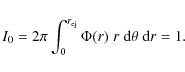
This function is normalized as follows
.
This function is normalized as follows
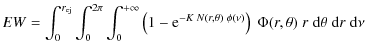
so that the total continuum flux emitted by the photodisk along the line of sight is equal to unity. If g(N,b) is the curve of growth for the given transition and Doppler parameter b, the equivalent width (EW) produced by an infinitesimal cloud column with cross section
If we neglect the small contribution by photons scattered by the cloud
into the line of sight, the total equivalent width is then computed
integrating the contribution of each single infinitesimal element over
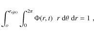
the photodisk (see Appendix A for the details):
![\begin{eqnarray*}EW(t)=\int_o^{r_{\rm ej(t)}} \int_0^{2\pi}
g[N(r,\theta),b(r,\theta)]\; \Phi(r,t)\; \;r \; {\rm d}\theta \; {\rm d}r.
\end{eqnarray*}](/articles/aa/full_html/2010/06/aa13959-09/img20.png)
So far we have considered the possibility that the Doppler parameter b can change across the cloud. However, in the lack of evidence for significant variations over the scales of interest (see for instance Welty & Fitzpatrick 2001), in the following we will assume that b is constant across the relevant portion of the cloud. We will briefly discuss the effects of a space-dependent Doppler parameter in Sect. 3.
With the aid of the outlined procedure, one can follow the time evolution of EW for any input cloud column density map, provided the photodisk's expansion law is known.
In the assumption of homologous expansion (see for instance
Jeffery &
Branch 1990),
the radius of the photosphere
![]() is
obtained
multiplying the photospheric velocity
is
obtained
multiplying the photospheric velocity
![]() by
the time t elapsed from the explosion. For
by
the time t elapsed from the explosion. For
![]() we
adopted a best fit to values computed via SYNOW modeling of the
spectroscopically normal SN 1994D, a standard type Ia
event (Branch et
al. 2005).
During the photospheric phase (t<100 days),
we
adopted a best fit to values computed via SYNOW modeling of the
spectroscopically normal SN 1994D, a standard type Ia
event (Branch et
al. 2005).
During the photospheric phase (t<100 days),
![]() is
well approximated by an exponential law, and the
best fit relation takes the following form:
is
well approximated by an exponential law, and the
best fit relation takes the following form:

where
As for the photodisk surface brightness profile, this was
computed
using a modified version of the spectrum synthesis code
SYNOW![]() (Branch et al. 2005). The
profile, obtained
from best fits of SN 1994D spectra for the Na I D
rest-frame
wavelength, rapidly drops at
(Branch et al. 2005). The
profile, obtained
from best fits of SN 1994D spectra for the Na I D
rest-frame
wavelength, rapidly drops at ![]() during the early phases
(see Fig. 2).
As time goes by, a significant fraction of
the flux (up to
during the early phases
(see Fig. 2).
As time goes by, a significant fraction of
the flux (up to ![]() 16%
on day +15) is emitted above the
photosphere, and it is due to scattering by the broad Na I D
doublet intrinsic to the SN (see for instance Jeffery & Branch
1990). At all
epochs,
16%
on day +15) is emitted above the
photosphere, and it is due to scattering by the broad Na I D
doublet intrinsic to the SN (see for instance Jeffery & Branch
1990). At all
epochs, ![]() for
for ![]() ,
which we used as the effective external boundary of the ejecta. To
include the time dependence we tabulated
,
which we used as the effective external boundary of the ejecta. To
include the time dependence we tabulated ![]() for a number of
epochs (-10, -4, +7, +15, +28 and +50 days from B
maximum) and
subsequently used a linear interpolation to derive the profile at any
given epoch. The time from B maximum light was
converted into tusing the rise time of
SN 1994D (18 days; Vacca & Leibundgut
1996). In view
of the lack of very early spectra, we
conservatively assumed that
for a number of
epochs (-10, -4, +7, +15, +28 and +50 days from B
maximum) and
subsequently used a linear interpolation to derive the profile at any
given epoch. The time from B maximum light was
converted into tusing the rise time of
SN 1994D (18 days; Vacca & Leibundgut
1996). In view
of the lack of very early spectra, we
conservatively assumed that ![]() for
for ![]() at t=0.
at t=0.
![\begin{figure}
\par\includegraphics[width=7cm,clip]{13959fg2.eps}\vspace{-3mm}
\end{figure}](/articles/aa/full_html/2010/06/aa13959-09/img30.png)
|
Figure 2: Surface brightness profiles derived from SYNOW best fits of SN 1994D spectra on four different epochs (-10, -4, +7 and +15 days from B maximum). |
| Open with DEXTER | |
2.1 Cloud generation
We explored two possible cases: i) an isolated, homogeneous,
spherical cloud with radius ![]() and offset
and offset ![]() with respect to the line of sight; ii) a patchy sheet with an
input spectrum for the
column density fluctuations.
with respect to the line of sight; ii) a patchy sheet with an
input spectrum for the
column density fluctuations.
In the first case, the column density profile is
![]() ,
where
,
where ![]() is the projected distance
from the cloud center (
is the projected distance
from the cloud center (
![]() ),
and N0 is the column
density corresponding to a ray going through the center of the
cloud. The average column density is
),
and N0 is the column
density corresponding to a ray going through the center of the
cloud. The average column density is
![]() N0. As
the case of an isolated, small cloud is probably quite unrealistic, it
may be rather regarded as a simplified model of an over-density on an
otherwise homogeneous sheet.
N0. As
the case of an isolated, small cloud is probably quite unrealistic, it
may be rather regarded as a simplified model of an over-density on an
otherwise homogeneous sheet.
For the patchy sheet we adopted a procedure similar to the one
described by Deshpande (2000).
Molecular clouds
(Elmegreen et al. 1996),
the diffuse ionized
component (Cordes et al. 1991),
and H I (Stanimirovic et al.
1999;
Deshpande et al.
2000)
have a fractal structure, characterized by a
power-law behavior. Therefore, if k=l0/l
is the wave-number
corresponding to a given spatial scale l (where l0
is the maximum
spatial scale under consideration), the power spectrum of the
fluctuations can be written as
![]() .
For the large
scale structure of H I in the SMC
.
For the large
scale structure of H I in the SMC
![]() 3
(Stanimirovic et al. 1999)
and
3
(Stanimirovic et al. 1999)
and ![]() for the cold atomic gas
in the Galaxy (Deshpande et al. 2000). Since
the
variations observed on scales of
for the cold atomic gas
in the Galaxy (Deshpande et al. 2000). Since
the
variations observed on scales of ![]() 100 AU and below can be
explained in terms of a single power spectrum description (Deshpande
2000), we
computed the column density maps using a
power-law with
100 AU and below can be
explained in terms of a single power spectrum description (Deshpande
2000), we
computed the column density maps using a
power-law with ![]() .
After generating a power spectrum map
P(kx,ky)
in the Fourier plane (with
k=(k2x
+k2y)1/2),
we
derive the real and imaginary parts of the Fourier transform of
N(x,y) using
.
After generating a power spectrum map
P(kx,ky)
in the Fourier plane (with
k=(k2x
+k2y)1/2),
we
derive the real and imaginary parts of the Fourier transform of
N(x,y) using
![]() as the modulus of the complex numbers,
while phases are generated as random numbers uniformly distributed
between 0 and 2
as the modulus of the complex numbers,
while phases are generated as random numbers uniformly distributed
between 0 and 2![]() .
The column density map is then obtained
anti-transforming into ordinary space. Given the radius of the
photosphere during the time interval typically covered by observations
(<400 AU), we adopt l0=1024 AU.
.
The column density map is then obtained
anti-transforming into ordinary space. Given the radius of the
photosphere during the time interval typically covered by observations
(<400 AU), we adopt l0=1024 AU.
Once the two-dimensional column density map is generated, it
is
re-normalized to have an average column density
![]() and
peak-to-peak fluctuations
and
peak-to-peak fluctuations ![]() (with
(with ![]() ).
An example cloud is presented in Fig. 1. If
).
An example cloud is presented in Fig. 1. If
![]() is the column density
difference between two points
separated by a distance l, the numerical
simulations show that for
is the column density
difference between two points
separated by a distance l, the numerical
simulations show that for
![]() the RMS value of
the RMS value of
![]() is
is ![]() 10% of the
maximum variation on the same spatial scale. Furthermore, the
differences at higher wave-numbers decrease proportionally to
10% of the
maximum variation on the same spatial scale. Furthermore, the
differences at higher wave-numbers decrease proportionally to
![]() ,
as predicted by theory (Deshpande
2000).
This implies that the fluctuations expected on
scales of 100 AU are
,
as predicted by theory (Deshpande
2000).
This implies that the fluctuations expected on
scales of 100 AU are ![]() 40% of those observed on
scales of 1000
AU, which for Na I can reach a few 1012 cm-2
(Andrews
et al. 2001).
Therefore, a significant amount of structure
is expected on spatial scales comparable to the typical photospheric
radius.
40% of those observed on
scales of 1000
AU, which for Na I can reach a few 1012 cm-2
(Andrews
et al. 2001).
Therefore, a significant amount of structure
is expected on spatial scales comparable to the typical photospheric
radius.
2.2 Measurement error estimates
The ability of detecting small EW variations hinges on the precision to which EWs can be measured. In turn, this relates to the instrumental setup and the signal-to-noise ratio SNR reached on the adjacent continuum per resolution element. To estimate the expected RMS uncertainty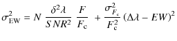
where
Table 1:
Estimated Equivalent Width RMS errors
![]() computed using Eq. (1)
( SNR = 100 and N=1012 cm-2).
computed using Eq. (1)
( SNR = 100 and N=1012 cm-2).
The results obtained for N=1012 cm-2,
and ![]() for different values of FWHM, b
(1, 3 and 5 km s-1corresponding
to EW of 58, 113 and 138 mÅ respectively),
and
for different values of FWHM, b
(1, 3 and 5 km s-1corresponding
to EW of 58, 113 and 138 mÅ respectively),
and
![]() are presented in
Table 1.
As the RMS
errors are inversely proportional to SNR, these
values can be
readily scaled to different signal-to-noise ratios. These results have
been checked against Monte-Carlo simulations and were found to be
consistent to within a few 0.1 mÅ. Incidentally, this
questions the
need for a revision of the Chalabaev & Maillard formula
discussed by
Vollmann & Eversberg (2006).
are presented in
Table 1.
As the RMS
errors are inversely proportional to SNR, these
values can be
readily scaled to different signal-to-noise ratios. These results have
been checked against Monte-Carlo simulations and were found to be
consistent to within a few 0.1 mÅ. Incidentally, this
questions the
need for a revision of the Chalabaev & Maillard formula
discussed by
Vollmann & Eversberg (2006).
In the following we will consider an equivalent width
variation
![]() detectable
if
detectable
if ![]() .
For
a typical case where FWHM=7 km s-1,
b=1 km s-1,
.
For
a typical case where FWHM=7 km s-1,
b=1 km s-1,
![]() Å
pix-1, and
Å
pix-1, and
![]() ,
this turns into a 5-
,
this turns into a 5-![]() detection limit
detection limit ![]() mÅ
(
mÅ
(
![]() mÅ
for b=5 km s-1).
mÅ
for b=5 km s-1).
3 Results of simulations
Although the model can be used for any inter-stellar absorption line, in the following we present the results obtained for Na I D2, because it is a strong transition, it falls in a region almost free of telluric absorption features, and in a spectral interval where most optical, high-resolution spectrographs have their maximum sensitivity.
![\begin{figure}
\par\includegraphics[width=7.8cm,clip]{13959fg3.eps}
\end{figure}](/articles/aa/full_html/2010/06/aa13959-09/img65.png)
|
Figure 3:
Examples of simulated Na I D2EW
variation as a function of time for a spherical, homogeneous
cloud with offset |
| Open with DEXTER | |
3.1 Isolated spherical cloud
Example EW evolutions for two different cloud
offsets ![]() (0 and 64
AU) and a number of cloud radii
(0 and 64
AU) and a number of cloud radii ![]() are presented in
Fig. 3
up to 2 months after maximum light. In
general, the maximum variability is expected when the cloud is close
to the center of the photodisk. The maximum variation is achieved for
cloud radii between 64 and 128 AU. Also, small clouds are
better
detected during the early phases (when their size is comparable to
that of the photosphere), while the detection of large clouds requires
a larger time span. If the cloud is too large (
are presented in
Fig. 3
up to 2 months after maximum light. In
general, the maximum variability is expected when the cloud is close
to the center of the photodisk. The maximum variation is achieved for
cloud radii between 64 and 128 AU. Also, small clouds are
better
detected during the early phases (when their size is comparable to
that of the photosphere), while the detection of large clouds requires
a larger time span. If the cloud is too large (
![]() AU), then
the EW variation is not sufficiently ample to be
detected. With a
minimum set of two observations taken 10 days apart in the pre-maximum
phases, for typical high-resolution setup, a 5-
AU), then
the EW variation is not sufficiently ample to be
detected. With a
minimum set of two observations taken 10 days apart in the pre-maximum
phases, for typical high-resolution setup, a 5-![]() detection
limit of 4.4 mÅ, b=1 km s-1
and
detection
limit of 4.4 mÅ, b=1 km s-1
and ![]() cm-2,
the simulations show that one is able to detect clouds with
cm-2,
the simulations show that one is able to detect clouds with
![]() between 16
and 128 AU up to a maximum offset of 64 AU. For
larger offsets the cloud starts to intersect the photodisk when its
size is too large and the corresponding covering factor is too
small. Besides implying probably unrealistic density contrasts,
increasing the column density does not enhance the detectability of a
small size cloud, since this rapidly becomes totally opaque. We note
that, while this causes the saturation of the covering factor, it does
not produce a saturated profile in the emerging absorption line.
between 16
and 128 AU up to a maximum offset of 64 AU. For
larger offsets the cloud starts to intersect the photodisk when its
size is too large and the corresponding covering factor is too
small. Besides implying probably unrealistic density contrasts,
increasing the column density does not enhance the detectability of a
small size cloud, since this rapidly becomes totally opaque. We note
that, while this causes the saturation of the covering factor, it does
not produce a saturated profile in the emerging absorption line.
A distinctive feature of small (
![]() AU), offset clouds
is an
EW growth followed by a decrease during the
pre-maximum light phase
(Fig. 3,
lower panel). This is due to the growth of
the covering factor as the photodisk starts intersecting the
off-centered knot. Once a maximum value is reached, the subsequent
increase in the photodisk size causes the covering factor to
drop. Although this mechanism can produce an absorption feature which
grows in strength and then disappears on timescales of a month, this
is expected to happen only during the pre-maximum epochs, when the
relative increase in the photodisk surface is very fast. Larger
clouds placed at larger offsets (
AU), offset clouds
is an
EW growth followed by a decrease during the
pre-maximum light phase
(Fig. 3,
lower panel). This is due to the growth of
the covering factor as the photodisk starts intersecting the
off-centered knot. Once a maximum value is reached, the subsequent
increase in the photodisk size causes the covering factor to
drop. Although this mechanism can produce an absorption feature which
grows in strength and then disappears on timescales of a month, this
is expected to happen only during the pre-maximum epochs, when the
relative increase in the photodisk surface is very fast. Larger
clouds placed at larger offsets (
![]() AU) produce features
which start appearing around maximum light, but keep steadily
increasing in strength up to several months after maximum.
AU) produce features
which start appearing around maximum light, but keep steadily
increasing in strength up to several months after maximum.
Finally, for central column densities (or density contrasts)
smaller
than ![]() cm-2, the EW variations are
always
below the detection limit.
cm-2, the EW variations are
always
below the detection limit.
3.2 Patchy clouds
Because of the stochastic geometry of the power-law clouds,
their
effects were evaluated using a statistical approach. For a given cloud
realization we computed ![]() and derived the absolute peak-to-peak
variation
and derived the absolute peak-to-peak
variation ![]() over the whole time interval -10 to +50 days.
To mimic a more realistic situation, we did this also on two
sub-sets of data-points including only post-maximum observations (0,
+10, +20, +30, +40, +50 and 0, +10, +20, +30 days). As
statistical
estimators we computed the median absolute peak-to-peak variation
over the full range (
over the whole time interval -10 to +50 days.
To mimic a more realistic situation, we did this also on two
sub-sets of data-points including only post-maximum observations (0,
+10, +20, +30, +40, +50 and 0, +10, +20, +30 days). As
statistical
estimators we computed the median absolute peak-to-peak variation
over the full range (
![]() ),
the semi-inter-quartile
range and the 99-th percentile (
),
the semi-inter-quartile
range and the 99-th percentile (
![]() ). For the three time
ranges we finally estimated the 5-
). For the three time
ranges we finally estimated the 5-![]() detection
probabilities Pt
(
detection
probabilities Pt
(
![]() ), P0
(
), P0
(![]() )
and
P30 (0
)
and
P30 (0
![]() ). The results are presented
in
Table 2
for different values of
). The results are presented
in
Table 2
for different values of ![]() ,
,
![]() and b.
For each parameter set 5000 cloud realizations
were computed (blank values indicate detection probabilities
and b.
For each parameter set 5000 cloud realizations
were computed (blank values indicate detection probabilities
![]() ).
).
![]() indicates the EW
corresponding to
indicates the EW
corresponding to ![]() and the input Doppler parameter.
and the input Doppler parameter.
Visual inspection of a number of realizations showed that the EW(t)curves
are smooth, with typical timescales of the order of 10 days.
The variation rate is systematically larger at early epochs and
decreases as time goes by. The simulations show that peak-to-peak
column density fluctuations smaller than 1011 cm-2
on a
scale of ![]() 1000 AU
do not produce any measurable effects. Even
with high (
1000 AU
do not produce any measurable effects. Even
with high (![]() 100)
signal-to-noise ratio observations, starting 10 days before
maximum and covering the first two months of the SN
evolution, the detection probability is below 2%. This grows
significantly when the fluctuations exceed
100)
signal-to-noise ratio observations, starting 10 days before
maximum and covering the first two months of the SN
evolution, the detection probability is below 2%. This grows
significantly when the fluctuations exceed
![]() cm-2.
Incidentally, this implies that SNe suffering higher
extinction are expected to display more pronounced variations (see
also Chugai 2008).
Because of the saturation effect, the EW
variations are more marked for larger values of the Doppler
parameter. Finally, for column densities exceeding
cm-2.
Incidentally, this implies that SNe suffering higher
extinction are expected to display more pronounced variations (see
also Chugai 2008).
Because of the saturation effect, the EW
variations are more marked for larger values of the Doppler
parameter. Finally, for column densities exceeding
![]() cm-2
the detection probability decreases due to line saturation.
cm-2
the detection probability decreases due to line saturation.
Table 2:
Results of Monte-Carlo simulations for power-law clouds with
![]() .
.
To study the effect of a spatially variable Doppler parameter,
we have
run a set of simulations in which b is allowed to
fluctuate around
the average value across the cloud. We have tentatively modeled the
Doppler parameter map using the same algorithm and spatial scales
spectrum adopted for the column density generation (see
Sect. 2.1).
We remark that this is not meant to reproduce
real physical conditions, but only to estimate the consequences of
velocity dispersion fluctuations (for instance, b
and ![]() were left completely independent). The MC runs (with 1
were left completely independent). The MC runs (with 1
![]() km s-1)
show that for
km s-1)
show that for ![]() cm-2
there is practically no difference with respect to the case
with constant Doppler parameter. The differences start to be
significant at
cm-2
there is practically no difference with respect to the case
with constant Doppler parameter. The differences start to be
significant at ![]() cm-2,
for which the
typical variations and detection probabilities become much larger.
cm-2,
for which the
typical variations and detection probabilities become much larger.
This was to be expected, since in the quasi-linear regime attained at low column densities the effect tends to average out. On the contrary, as one enters the non-linear part of the curve of growth, the largest variations are produced by the regions of the cloud where the Doppler parameter is higher (i.e. less subject to saturation), thus skewing the distribution towards more marked EW fluctuations. The exact behavior depends on the way the velocity dispersion varies across the cloud and how this (if any) relates to the column density fluctuations. However, the conclusion that a variable Doppler parameter enhances the detection probability is of general validity.
4 Discussion and conclusions
The simulations presented in this paper indicate that marked time
effects on the measured EWs are expected for small
(
![]() AU), isolated clouds
with
AU), isolated clouds
with
![]() cm-2
and for small offsets (
cm-2
and for small offsets (
![]() AU). However, the
existence
of such structures is seriously questioned in terms of pressure
equilibrium arguments and the yet unknown processes that would produce
them (see Heiles 1997,
and references therein). Frail et al. (1994) detected
maximum
AU). However, the
existence
of such structures is seriously questioned in terms of pressure
equilibrium arguments and the yet unknown processes that would produce
them (see Heiles 1997,
and references therein). Frail et al. (1994) detected
maximum ![]() variations
that range from
variations
that range from ![]() 1019
to
1019
to ![]() cm-2
on scales between 5 and 100 AU. For a Galactic
Na I/H I ratio
(Ferlet et al.
1985) this
turns into
cm-2
on scales between 5 and 100 AU. For a Galactic
Na I/H I ratio
(Ferlet et al.
1985) this
turns into ![]() between
between
![]() and
and
![]() cm-2.
These large
changes have been interpreted as arising within ubiquitously
distributed small structures. However, this picture has been
questioned by Deshpande (2000),
who has convincingly
shown that the observations are consistent with a single power-law
description of the ISM, down to AU scales. In these
circumstances,
peak-to-peak variations
cm-2.
These large
changes have been interpreted as arising within ubiquitously
distributed small structures. However, this picture has been
questioned by Deshpande (2000),
who has convincingly
shown that the observations are consistent with a single power-law
description of the ISM, down to AU scales. In these
circumstances,
peak-to-peak variations
![]() cm-2are
expected on scales of
cm-2are
expected on scales of ![]() AU.
Our calculations (see
Table 2)
show that for a type Ia SN observed under the
most favorable conditions (
AU.
Our calculations (see
Table 2)
show that for a type Ia SN observed under the
most favorable conditions (
![]() on all epochs, spanning
from -10 to +50 days) these would appear in less than 10% of
the
cases for
on all epochs, spanning
from -10 to +50 days) these would appear in less than 10% of
the
cases for ![]() km s-1.
This fraction increases to
km s-1.
This fraction increases to ![]() 80%
for
80%
for ![]() km
s-1, but in all cases it is
km
s-1, but in all cases it is
![]() mÅ.
These small variations imply negligible changes in E(B-V),
but
can have some effect on observing programmes studying the evolution of
Na I features possibly arising in the
circumstellar environment
of type Ia progenitors (Patat et al. 2007; Simon
et al. 2009).
However, we note that these values are more than
a factor of 10 smaller than the Na I D
variations detected in
the type Ia SN 2006X (Patat et al. 2007), which were
attributed to the ionization effects induced by the SN on its
circum-stellar environment. In contrast, no statistically significant
variations were detected for the CN, CH, CH+, Ca
I lines and
DIBs associated to an interstellar cloud in the host galaxy (Patat
et al. 2007;
Cox & Patat 2008).
In the only other well
studied case published so far (SN 2007le), the EW
of four Na I
D components remained constant to within a few mÅ during six
epochs spanning about 3 months (Simon et al. 2009). In this
time range
mÅ.
These small variations imply negligible changes in E(B-V),
but
can have some effect on observing programmes studying the evolution of
Na I features possibly arising in the
circumstellar environment
of type Ia progenitors (Patat et al. 2007; Simon
et al. 2009).
However, we note that these values are more than
a factor of 10 smaller than the Na I D
variations detected in
the type Ia SN 2006X (Patat et al. 2007), which were
attributed to the ionization effects induced by the SN on its
circum-stellar environment. In contrast, no statistically significant
variations were detected for the CN, CH, CH+, Ca
I lines and
DIBs associated to an interstellar cloud in the host galaxy (Patat
et al. 2007;
Cox & Patat 2008).
In the only other well
studied case published so far (SN 2007le), the EW
of four Na I
D components remained constant to within a few mÅ during six
epochs spanning about 3 months (Simon et al. 2009). In this
time range ![]() changed approximately from 100 to 400 AU, and
the lack of evolution is in line with the predictions of our model for
a power spectrum ISM and definitely excludes the presence of small,
isolated clouds with sizes comparable to
changed approximately from 100 to 400 AU, and
the lack of evolution is in line with the predictions of our model for
a power spectrum ISM and definitely excludes the presence of small,
isolated clouds with sizes comparable to
![]() .
Although the
available data are still scanty, the multi-epoch, high-resolution
campaigns which are being conducted for the study of type Ia
progenitors will provide a more statistically significant sample.
.
Although the
available data are still scanty, the multi-epoch, high-resolution
campaigns which are being conducted for the study of type Ia
progenitors will provide a more statistically significant sample.
All the discussion so far is based on the assumption that the
physical
conditions of the ISM are not modified by the SN explosion, so
that
all variations in the absorption lines are due to pure geometric
effects. Indeed, a type Ia SN can produce changes in the
ionization
balance of low-ionization species (like Na I
or K I) up
to quite large distances, of the order of 10 pc (Patat
et al. 2007;
Chugai 2008;
Simon et al. 2009).
Given the UV flux predicted for these distances
(Simon et al. 2009),
the ionization timescale of Na I
is expected to be about 120 days. Since the electron density
in the
ISM is low, the recombination time is extremely long. Therefore, under
the assumption of a constant ionizing field, one would expect the
amount of neutral Na to decrease with timescales of several months,
hence mimiking small scale structure effects. However, the UV flux of
a type Ia SN decreases significantly after maximum
light (a factor
![]() 20 in the
first 40 days; Brown et al. 2009) implying
that the maximum distance is probably less than 10 pc. Given the range
of possible distances to an inter-stellar cloud within the host galaxy,
this
suggests that significant Na I column
density variations in the
ISM induced by the SN radiation field are improbable.
20 in the
first 40 days; Brown et al. 2009) implying
that the maximum distance is probably less than 10 pc. Given the range
of possible distances to an inter-stellar cloud within the host galaxy,
this
suggests that significant Na I column
density variations in the
ISM induced by the SN radiation field are improbable.
Another important fact is that, because of the much higher ionization potential of Ca II, and the strong UV line blocking present in type Ia spectra, the EW of the ubiquitous H&K lines becomes insensitive to the SN radiation field already at distances of a few 0.1 pc (Simon et al. 2009). In contrast, in the case of a geometrical origin, all species are expected to show synchronous variations, although possibly with different amplitudes and time scales (Lauroesch & Meyer 2003). Therefore, a comparison between the behaviors of Na I and Ca II should allow one to disentangle between geometrical and ionization effects, similar to what has been proposed by Patat et al. (2007).
The method we presented enables the study of small scale structure in the extragalactic ISM, which is out of reach for any of the techniques deployed so far. In this respect we note that the same method can be in principle applied to the Galactic ISM to study its sub-AU structure, for which no direct measurements are available yet. Although probably requiring very high signal-to-noise ratios, this technique might put important constraints on the very small scale structure. In this article we have discussed the case of the strong, easily detectable Na I D lines. However, other weaker lines (e.g., K I, Ca I, Ca II) can be used, especially when the Na I D lines are saturated. In general, the simultaneous study of different atomic/diatomic lines along the lines of sight to SNe will contribute to get a more detailed picture of the physical conditions of the ISM in the small scales regime.
Appendix A: Calculation of composite equivalent width
Let us consider an extended photodisk, a cloud placed in front of it
and an absorption line with profile function ![]() ,
normalized so that
,
normalized so that
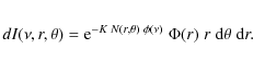
If N is the space-dependent column density of the cloud (atoms cm-2) for the atomic species under consideration, the monochromatic line optical depth is
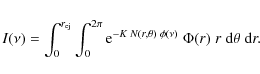
With these settings, the monochromatic intensity contributed by the infinitesimal photodisk element
For a distant observer, to whom the photodisk will appear as an unresolved source, the total line intensity profile
Given the definition of equivalent width
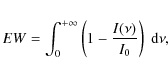
the composite equivalent width can be expressed as follows:
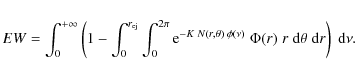
Because of the normalization of
Now, the inner integral is the equivalent width one would observe if the physical system were composed only by the infinitesimal cloud element
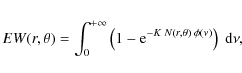
which implies that the composite equivalent width is the weighted sum of the equivalent widths produced within each infinitesimal cloud element. If g(N,b) is the curve of growth for the given transition (where b is the Doppler parameter that characterizes the line profile), then Eq. (A.1) can be reformulated as:
![$\displaystyle EW=\int_0^{r_{\rm ej}}\int_0^{2\pi}
g[N(r,\theta),b(r,\theta)] \; \Phi(r,\theta)\;r\;{\rm d}\theta\;{\rm d}r.$](/articles/aa/full_html/2010/06/aa13959-09/img113.png)
Acknowledgements
The authors wish to thank L. Tacconi-Garman, S. Stanimirovic and A. Deshpande for their kind help. The authors are also grateful to an anonymous referee for the useful comments and suggestions.
References
- André, M. K., Le Petit, F., Sonnentrucker, P., et al. 2004, A&A, 422, 483 [NASA ADS] [CrossRef] [EDP Sciences] [Google Scholar]
- Andrews, S. M., Meyer, D. M., & Lauroesch, J. T. 2001, ApJ, 552, L73 [NASA ADS] [CrossRef] [Google Scholar]
- Branch, D., Baron, E., Hall, N., et al. 2005, PASP, 117, 545 [NASA ADS] [CrossRef] [Google Scholar]
- Brown, P. J., Holland, S. T., Immler, S., et al. 2009, ApJ, 137, 4517 [Google Scholar]
- Chalabaev, A., & Maillard, J. P. 1983, A&A, 127, 279 [NASA ADS] [Google Scholar]
- Chugai, N. N. 2008, Astron. Lett., 34, 389 [NASA ADS] [CrossRef] [Google Scholar]
- Cordes, J. M., Weisberg, J. M., Frail, D. A., Spangler, S. R., & Ryan, M. 1991, Nature, 354, 121 [NASA ADS] [CrossRef] [Google Scholar]
- Cordiner, M., Sarre, P., & Fossey, S. 2005, AAO News Letter, 107, 9 [Google Scholar]
- Cox, N. L.J., & Patat, F. 2008, A&A, 485, L9 [NASA ADS] [CrossRef] [EDP Sciences] [Google Scholar]
- Crawford, I. A., Howarth, I. D., Ryder, S. D., & Stathakis, R. A. 2000, MNRAS, 319 L1 [NASA ADS] [CrossRef] [Google Scholar]
- Crawford, I. A. 2003, Ap&SS, 285, 661 [NASA ADS] [CrossRef] [Google Scholar]
- Deshpande, A. A. 2000, MNRAS, 317, 199 [NASA ADS] [CrossRef] [Google Scholar]
- Deshpande, A. A., Dwarakanath, K. S., & Goss, W. M. 2000, ApJ, 543, 227 [NASA ADS] [CrossRef] [Google Scholar]
- Dickey, J. M., & Lockman, F. J. 1990, ARA&A, 28, 215 [NASA ADS] [CrossRef] [MathSciNet] [Google Scholar]
- Diamond, P. J., Goss, W. M., Romney, J. D., et al. 1989, ApJ, 347, 302 [NASA ADS] [CrossRef] [Google Scholar]
- Dieter, N. H., Welch, W. J., & Romney, J. D. 1976, ApJ, 206, L113 [NASA ADS] [CrossRef] [Google Scholar]
- Elmegreen, B. G., & Falgarone, E. 1996, ApJ, 471, 816 [NASA ADS] [CrossRef] [Google Scholar]
- Ferlet, R., Vidal-Madjar, A., & Gry, C. 1985, ApJ, 298, 838 [NASA ADS] [CrossRef] [Google Scholar]
- Frail, D. A., Cordes, J. M., Hankins, T. H., & Weisberg, J. M. 1991, ApJ, 382, 168 [NASA ADS] [CrossRef] [Google Scholar]
- Frail, D. A., Weisberg, J. M., Cordes, J. M., & Mathers, A. 1994, ApJ, 436, 144 [NASA ADS] [CrossRef] [Google Scholar]
- Haverkorn, M., & Goss, W. M. 2007, SINS - Small Ionized and Neutral Structures in the Diffuse Interstellar Medium, ed. Haverkorn, M., & Goss, W. M. (San Francisco: ASP), ASP Conf. Ser., 365 [Google Scholar]
- Heiles, C. 1997, ApJ, 481, 193 [NASA ADS] [CrossRef] [Google Scholar]
- Jeffery, D., & Branch, D. 1990, Jerusalem Winter School for Theoretical Physics, Supernovae, ed. J. C. Wheeler, T. Piran, & S. Weinberg (Singapore: World Scientific Publishing Co.), 149 [Google Scholar]
- Lauroesch, J. T., & Meyer, D. M. 2003, ApJ, 591, L123 [NASA ADS] [CrossRef] [Google Scholar]
- Lauroesch, J. T. 2007, in SINS - Small Ionized and Neutral Structures in the Diffuse Interstellar Medium, ed. M. Haverkorn, & W. M. Goss (San Francisco: ASP), ASP Conf. Ser., 365, 40 [Google Scholar]
- Mazzali, P. A., & Lucy, L. B. 1993, A&A, 279, 447 [NASA ADS] [Google Scholar]
- Pan, K., Federman, S. R., Cunha, K., Smith, V. V., & Welty, D. E. 2004, ApJS, 151, 313 [NASA ADS] [CrossRef] [Google Scholar]
- Patat, F., Chandra, P., Chevalier, R., et al. 2007, Science, 317, 924 [NASA ADS] [CrossRef] [EDP Sciences] [PubMed] [Google Scholar]
- Rollinde, E., Boissé, P., Federman, S. R., & Pan, K. 2003, A&A, 401, 215 [NASA ADS] [CrossRef] [EDP Sciences] [Google Scholar]
- Simon, J. D., Gal-Yam, A., Gnat, O., et al. 2009 ApJ, 702, 1157 [Google Scholar]
- Stanimirovic, S., Stavely-Smith, S. L., Dickey, J. M., Sault, R. J., & Snowden, S. L. 1999, MNRAS, 302, 417 [NASA ADS] [CrossRef] [Google Scholar]
- Vacca, W. D., & Leibundgut, B. 1996, ApJ, 471, L37 [NASA ADS] [CrossRef] [Google Scholar]
- Van Loon, J. Th., Smith, K. T., McDonald, I., et al. 2009, MNRAS, 399, 195 [NASA ADS] [CrossRef] [Google Scholar]
- Vollmann, K., & Eversberg, T. 2006, Astron. Nachr., 327, No.9, 862 [NASA ADS] [CrossRef] [Google Scholar]
- Wang, L., & Wheeler, J. C. 2008, ARA&A, 46, 433 [NASA ADS] [CrossRef] [Google Scholar]
- Weisberg, J. M., & Stanimirovic, S. 2007, in SINS - Small Ionized and Neutral Structures in the Diffuse Interstellar Medium, ed. M. Haverkorn, & W. M. Goss (San Francisco: ASP), ASP Conf. Ser., 365, 28 [Google Scholar]
- Welty, D. E., & Fitzpatrick, E. L. 2001, ApJ, 551, L175 [NASA ADS] [CrossRef] [Google Scholar]
Footnotes
- ... interest
![[*]](/icons/foot_motif.png)
- We assume
 has no azimuthal
dependence, i.e. that the SN is spherically symmetric. For a type Ia
SN this is a reasonable assumption (Wang & Wheeler
2008).
has no azimuthal
dependence, i.e. that the SN is spherically symmetric. For a type Ia
SN this is a reasonable assumption (Wang & Wheeler
2008).
- ...
SYNOW
- Note that SYNOW, like some other SN spectrum synthesis codes (see e.g. Mazzali & Lucy 1993), has zero limb darkening.
- ... value
- For the purposes of measuring the EW of an inter-stellar line, the continuum definition in a SN spectrum is much easier than in a stellar spectrum, where the presence of other intrinsic features may contaminate the adjacent regions.
All Tables
Table 1:
Estimated Equivalent Width RMS errors
![]() computed using Eq. (1)
( SNR = 100 and N=1012 cm-2).
computed using Eq. (1)
( SNR = 100 and N=1012 cm-2).
Table 2:
Results of Monte-Carlo simulations for power-law clouds with
![]() .
.
All Figures
|
|
Figure 1:
Relevant quantities used in the text. The underlying column density map
was generated using a power-law spectrum with
|
| Open with DEXTER | |
| In the text | |
|
|
Figure 2: Surface brightness profiles derived from SYNOW best fits of SN 1994D spectra on four different epochs (-10, -4, +7 and +15 days from B maximum). |
| Open with DEXTER | |
| In the text | |
|
|
Figure 3:
Examples of simulated Na I D2EW
variation as a function of time for a spherical, homogeneous
cloud with offset |
| Open with DEXTER | |
| In the text | |
Copyright ESO 2010
Current usage metrics show cumulative count of Article Views (full-text article views including HTML views, PDF and ePub downloads, according to the available data) and Abstracts Views on Vision4Press platform.
Data correspond to usage on the plateform after 2015. The current usage metrics is available 48-96 hours after online publication and is updated daily on week days.
Initial download of the metrics may take a while.