| Issue |
A&A
Volume 514, May 2010
|
|
|---|---|---|
| Article Number | A77 | |
| Number of page(s) | 14 | |
| Section | Extragalactic astronomy | |
| DOI | https://doi.org/10.1051/0004-6361/200913833 | |
| Published online | 26 May 2010 | |
Submillimeter galaxies behind the Bullet cluster (1E 0657-56)
D. Johansson1 - C. Horellou1 - M. W. Sommer2 - K. Basu3,2 - F. Bertoldi2 - M. Birkinshaw4 - K. Lancaster4 - O. Lopez-Cruz5 - H. Quintana6
1 - Onsala Space Observatory, Chalmers University of
Technology, 439 92 Onsala, Sweden
2 - Argelander-Institut für
Astronomie, Auf dem Hügel 71, 53121 Bonn, Germany
3 - Max-Planck Institut für Radioastronomie, Auf dem Hügel 69, 53121 Bonn, Germany
4 - Department of Physics, University of Bristol, Tyndall Avenue, Bristol BS8 1TL, UK
5 -
Instituto Nacional de Astrofísica, Optica y Electrónica (INAOE),
Tonantzintla, Puebla 72840, Mexico
6 - Departamento de Astronomía
y Astrofísica, Pontificia Universidad Católica de Chile, Casilla 306, Santiago 22, Chile
Received 9 December 2009 / Accepted 19 February 2010
Abstract
Context. Clusters of galaxies are effective gravitational
lenses able to magnify background galaxies and making it possible to
probe the fainter part of the galaxy population. Submillimeter
galaxies, which are believed to be star-forming galaxies at typical
redshifts of 2 to 3, are a major contaminant to the extended
Sunyaev-Zeldovich (SZ) signal of galaxy clusters. For a proper
quantification of the SZ signal the contribution of submillimeter
galaxies needs to be quantified.
Aims. The aims of this study are to identify submillimeter
sources in the field of the Bullet cluster (1E 0657-56), a massive
cluster of galaxies at
![]() ,
measure their flux densities at 870
,
measure their flux densities at 870 ![]() m, and search for counterparts at other wavelengths to constrain their properties.
m, and search for counterparts at other wavelengths to constrain their properties.
Methods. We carried out deep observations of the submillimeter continuum emission at 870 ![]() m
using the Large APEX BOlometer CAmera (LABOCA) on the Atacama
Pathfinder EXperiment (APEX) telescope. Several numerical techniques
were used to quantify the noise properties of the data and extract
sources.
m
using the Large APEX BOlometer CAmera (LABOCA) on the Atacama
Pathfinder EXperiment (APEX) telescope. Several numerical techniques
were used to quantify the noise properties of the data and extract
sources.
Results. In total, seventeen sources were found. Thirteen of
them lie in the central 10 arcmin of the map, which has a pixel
sensitivity of 1.2 mJy per 22'' beam. After correction for flux
boosting and gravitational lensing, the number counts are consistent
with published submm measurements. Nine of the sources have infrared
counterparts in Spitzer maps. The strongest submm detection coincides
with a source previously reported at other wavelengths, at an estimated
redshift
![]() .
If the submm flux arises from two images of a galaxy magnified by a
total factor of 75, as models have suggested, its intrinsic flux
would be around 0.6 mJy, consistent with an intrinsic luminosity
below
.
If the submm flux arises from two images of a galaxy magnified by a
total factor of 75, as models have suggested, its intrinsic flux
would be around 0.6 mJy, consistent with an intrinsic luminosity
below
![]() .
.
Key words: galaxies: individual: MMJ065837-5557.0 - galaxies: clusters: individual: 1E 0657-56 - submillimeter: galaxies - infrared: galaxies - cosmology: observations
1 Introduction
The large concentrations of mass (up to
![]() )
on angular
scales of a few arcminutes in galaxy clusters act as natural
gravitational lenses capable of magnifying background galaxies that
would be too dim to be detectable otherwise. In the mm and submm
wavebands, lensing by galaxy clusters makes it possible to probe the
fainter part of the brightness distribution of the so-called
submillimeter galaxies (SMGs), which are believed to be dusty
high-redshift star-forming galaxies (Blain 1997).
)
on angular
scales of a few arcminutes in galaxy clusters act as natural
gravitational lenses capable of magnifying background galaxies that
would be too dim to be detectable otherwise. In the mm and submm
wavebands, lensing by galaxy clusters makes it possible to probe the
fainter part of the brightness distribution of the so-called
submillimeter galaxies (SMGs), which are believed to be dusty
high-redshift star-forming galaxies (Blain 1997).
Pioneering observations of SMGs at 450 and ![]() m were done using
SCUBA on the James Clerk Maxwell Telescope. The first observations
toward two massive clusters at
m were done using
SCUBA on the James Clerk Maxwell Telescope. The first observations
toward two massive clusters at
![]() resulted in the
detection of a total of six sources above the noise level of 2 mJy/beam at
resulted in the
detection of a total of six sources above the noise level of 2 mJy/beam at ![]() m (Smail et al. 1997). The authors estimated the surface density of the sources to be three
orders of magnitude larger than the expectation from a non-evolving
model using the local IRAS
m (Smail et al. 1997). The authors estimated the surface density of the sources to be three
orders of magnitude larger than the expectation from a non-evolving
model using the local IRAS ![]() m luminosity function. Those
observations provided evidence for the presence of a large number of
actively star-forming galaxies at high redshift, which might be the
counterparts of the luminous and ultraluminous infrared galaxies
observed in the local universe (e.g. Sanders & Mirabel 1996).
m luminosity function. Those
observations provided evidence for the presence of a large number of
actively star-forming galaxies at high redshift, which might be the
counterparts of the luminous and ultraluminous infrared galaxies
observed in the local universe (e.g. Sanders & Mirabel 1996).
At redshifts beyond one, the flux density of a redshifted infrared-luminous galaxy is largely redshift-independent: its decrease with an increasing distance is compensated by the steep rise in the mm and submm due to the redshifted spectral energy distribution (Blain & Longair 1993). During the last decade, several hundreds of SMGs have been discovered using bolometer arrays, mostly SCUBA (e.g. Blain 1998; Coppin et al. 2006; Borys et al. 2003), and more recently MAMBO at 1.2 mm and AzTEC at 1.1 mm (Austermann et al. 2010; Scott et al. 2008; Bertoldi et al. 2007). The mm/submm galaxy population is the subject of many multi-wavelength studies (see the review by Blain et al. 2002). The median redshift of SMGs with known redshifts is around 2-3 (Smail et al. 2000).
So far, only a handful of massive galaxy clusters have been mapped in the submm, and most of them are clusters in the northern hemisphere observed with SCUBA. Observation of seven massive clusters with a sensitivity of 2 mJy/beam provided a catalogue of 17 submm sources brighter than the 50% completeness limit (Smail et al. 1998). Nine other cluster fields in the redshift range 0.2-0.8 were observed with a similar sensitivity, resulting in the detection of 17 new submm sources (Chapman et al. 2002). Deeper observations with a 3-sigma limit of 1.5-2 mJy/beam of three massive clusters probed the sub-mJy number counts, because of the gravitational magnification of the clusters. (Cowie et al. 2002). Knudsen et al. (2008) targeted twelve clusters and the New Technology Telescope Deep Field. They detected 59 sources (some of them being multiple images of the same galaxy), and determined that seven of them have sub-mJy lensing-corrected flux densities.
The LABOCA bolometer camera on APEX has been used to survey the
870
![]() emission in a protocluster at
emission in a protocluster at
![]() (Beelen et al. 2008) and the Extended Chandra Deep Field South
Weiß et al. (2009). Nord et al. (2009)
observed the Sunyaev-Zeldovich (SZ) increment toward the massive
cluster Abell 2163 and noted one bright point source. This is a
good candidate for an SMG lensed by the cluster.
(Beelen et al. 2008) and the Extended Chandra Deep Field South
Weiß et al. (2009). Nord et al. (2009)
observed the Sunyaev-Zeldovich (SZ) increment toward the massive
cluster Abell 2163 and noted one bright point source. This is a
good candidate for an SMG lensed by the cluster.
The Bullet cluster (1E 0657-56) at
![]() is one of the most
massive galaxy clusters known to date
(see Markevitch et al. 2002; Springel & Farrar 2007). A bright
millimeter source was recently discovered in the Bullet cluster field
and identified as the lensed image of a background galaxy at a
redshift of about 2.7 (Wilson et al. 2008, hereafter W08).
The source happens to lie close to a critical line of the lens,
causing a large flux amplification. The observations were performed
with the AzTEC bolometer camera on the 10-m ASTE telescope in the
Atacama desert in Chile, which provides an angular resolution of
30'' at 1.1 mm wavelength. A doubly lensed source at the same
location had been previously identified in Hubble Space Telescope
(HST) maps and was used, together with other multiply lensed
galaxies and a large number of weakly lensed sources, to obtain a
calibrated map of the projected mass distribution of the Bullet
cluster (Bradac et al. 2006). Recently, Gonzalez et al. (2009)
identified a third image by analyzing maps in the optical (HST), and
in the near- and mid-infrared (Magellan and Spitzer). By fitting the
spectral energy distribution (SED) of a starburst galaxy to the
observations, they also inferred a redshift of about 2.7. Their
lensing model gave a magnification of 10-50 for the three images.
is one of the most
massive galaxy clusters known to date
(see Markevitch et al. 2002; Springel & Farrar 2007). A bright
millimeter source was recently discovered in the Bullet cluster field
and identified as the lensed image of a background galaxy at a
redshift of about 2.7 (Wilson et al. 2008, hereafter W08).
The source happens to lie close to a critical line of the lens,
causing a large flux amplification. The observations were performed
with the AzTEC bolometer camera on the 10-m ASTE telescope in the
Atacama desert in Chile, which provides an angular resolution of
30'' at 1.1 mm wavelength. A doubly lensed source at the same
location had been previously identified in Hubble Space Telescope
(HST) maps and was used, together with other multiply lensed
galaxies and a large number of weakly lensed sources, to obtain a
calibrated map of the projected mass distribution of the Bullet
cluster (Bradac et al. 2006). Recently, Gonzalez et al. (2009)
identified a third image by analyzing maps in the optical (HST), and
in the near- and mid-infrared (Magellan and Spitzer). By fitting the
spectral energy distribution (SED) of a starburst galaxy to the
observations, they also inferred a redshift of about 2.7. Their
lensing model gave a magnification of 10-50 for the three images.
![\begin{figure}
\par\mbox{\includegraphics[width=8cm,clip]{13833f1_1.eps} \includegraphics[width=8cm,clip]{13833f1_2.eps} }
\end{figure}](/articles/aa/full_html/2010/06/aa13833-09/img18.png)
|
Figure 1:
Left: layout of the bolometers on the
LABOCA array. Each circle represents one bolometer that was active
at the time of the observations. The two rectangles illustrate the
sizes of the two raster+spiral scanning pattern for one bolometer
(solid line-small pattern, dashed line-large
pattern). Right: movement pattern for one bolometer during
the large scanning pattern. This pattern has a
|
| Open with DEXTER | |
In this paper we present results of observations of the Bullet cluster
field at a wavelength of 870
![]() using the
LABOCA bolometer camera. At that wavelength, the emission is a
combination of extended signal due to the Sunyaev-Zeldovich effect by
the hot intracluster gas and of point sources, which are potential
high-redshift star-forming galaxies. Recovery of the extended SZ
signal from the LABOCA data (the SZ increment) requires a different
data reduction and will be presented in a subsequent paper. The
SZ decrement from the Bullet cluster has been mapped by
e.g. Halverson et al. (2009) with the APEX-SZ instrument, operating
at 2 mm. This paper is organized as follows: the observations are
presented in Sect. 2.1 and the data reduction in
Sect. 3; the results are presented and
discussed in Sects. 4 and 5.
using the
LABOCA bolometer camera. At that wavelength, the emission is a
combination of extended signal due to the Sunyaev-Zeldovich effect by
the hot intracluster gas and of point sources, which are potential
high-redshift star-forming galaxies. Recovery of the extended SZ
signal from the LABOCA data (the SZ increment) requires a different
data reduction and will be presented in a subsequent paper. The
SZ decrement from the Bullet cluster has been mapped by
e.g. Halverson et al. (2009) with the APEX-SZ instrument, operating
at 2 mm. This paper is organized as follows: the observations are
presented in Sect. 2.1 and the data reduction in
Sect. 3; the results are presented and
discussed in Sects. 4 and 5.
Throughout the paper, we adopt the following cosmological parameters:
a Hubble constant H0 = 70 km s-1 Mpc-1, a matter density
parameter
![]() ,
and a dark energy density parameter
,
and a dark energy density parameter
![]() .
The redshift z=0.296 of the Bullet
cluster corresponds to an angular-diameter distance of 910 Mpc and a
scale of 4.41 kpc/arcsec.
.
The redshift z=0.296 of the Bullet
cluster corresponds to an angular-diameter distance of 910 Mpc and a
scale of 4.41 kpc/arcsec.
2 Observations
2.1 Submillimeter
The observations![]() were carried out in September, October and
November 2007 using LABOCA (Large APEX BOlometer CAmera,
Siringo et al. 2009) on the APEX telescope
were carried out in September, October and
November 2007 using LABOCA (Large APEX BOlometer CAmera,
Siringo et al. 2009) on the APEX telescope![]() (Güsten et al. 2006). LABOCA is a 295-element receiver operating at a
central frequency of 345 GHz with a bandwidth of 60 GHz. At the time
of our observations, about 250 bolometers were used. The mean
point-source sensitivity of those bolometers was
78
(Güsten et al. 2006). LABOCA is a 295-element receiver operating at a
central frequency of 345 GHz with a bandwidth of 60 GHz. At the time
of our observations, about 250 bolometers were used. The mean
point-source sensitivity of those bolometers was
78
![]() .
The angular resolution was
.
The angular resolution was
![]() and the field-of-view was
and the field-of-view was
![]() .
The layout of the bolometer
array is illustrated in Fig. 1. A total of 25 h of
observing time was spent, including pointing and calibration. The
weather conditions were varying, with an amount of precipitable water
vapor ranging from 0.5 to 2.0 mm.
.
The layout of the bolometer
array is illustrated in Fig. 1. A total of 25 h of
observing time was spent, including pointing and calibration. The
weather conditions were varying, with an amount of precipitable water
vapor ranging from 0.5 to 2.0 mm.
LABOCA uses feed horn antennas and their physical size limits the spacing of the bolometers on the array. LABOCA is therefore not fully sampling the sky, so the telescope has to be moved to sample the sky such that the resulting map meets the Nyquist criterion. The scanning pattern does not only ``fill the gaps'' between bolometers, it also modulates the astronomical signal into a range of spatial frequencies which facilitates filtering of 1/f-type noise (instrumental and sky noise).
2.1.1 Scanning patterns
We used two different scanning patterns, as illustrated in Fig. 1. Both are a combination of Archimedian spirals with a duration of 35 s, centered on a four-point raster.
- During the first observing session, we used a compact scanning
pattern: the four points were separated by
 in azimuth and
elevation, each point marking the center of a spiral with a minimum
radius of
in azimuth and
elevation, each point marking the center of a spiral with a minimum
radius of
 and winding out with a radial speed of
 and an angular speed of
 .
The spirals thus ranged from
.
The spirals thus ranged from
 to about
 in radius, with a scanning speed between
 and
and
 .
.
- During the second observing session, a larger scanning pattern was
used to facilitate the retrieval of the extended
SZ signal. The four raster points were separated by
 in azimuth and elevation, and the spirals had a minimum radius
R0=
120'' and radial and angular speeds of
in azimuth and elevation, and the spirals had a minimum radius
R0=
120'' and radial and angular speeds of
 ,
.
The spirals thus ranged from 120 to
,
.
The spirals thus ranged from 120 to
 in radius, with a scanning speed between 3 and
 .
.
2.1.2 Pointing, focus and calibration
The pointing accuracy was checked by repeated observations of the
nearby source PKS 0537-441. This is a variable source; during our
observations, its mean flux density was ![]() 3 Jy. The source was
scanned in a tight spiral and the data were reduced and made into a
map using the BoA software (see Sect. 3). A
two-dimensional Gaussian was fitted to the pointing source, and the
telescope's pointing was updated using offsets from the fit. The
pointing was stable within
3 Jy. The source was
scanned in a tight spiral and the data were reduced and made into a
map using the BoA software (see Sect. 3). A
two-dimensional Gaussian was fitted to the pointing source, and the
telescope's pointing was updated using offsets from the fit. The
pointing was stable within
![]() .
.
The focus was checked at least twice during every observing session by observing a planet (Venus, Saturn or Mars). The subreflector was moved in small increments in each of the three cartesian directions while the telescope tracked the source. The optimum focus position in each direction was determined by fitting a curve to the observed points, and the subreflector was finally moved to the position corresponding to the maximum of the curve.
The absolute flux calibration of LABOCA is supposed to be accurate to 10% (Siringo et al. 2009). We verified this by daily observations of Uranus.
The atmospheric attenuation was determined from continuous scans in elevation at a fixed azimuth (``skydips''), and from radiometer measurements (Siringo et al. 2009).
2.2 Infrared
In Sect. 5.1 we describe a search for infrared counterparts to the detected submm sources in Spitzer maps. We now describe the data that was used for that comparison.
Spitzer IRAC and MIPS of the Bullet cluster field were acquired from the Spitzer data archive. Both the IRAC and MIPS data were taken under program ID 40593 (PI: Gonzalez). The Spitzer data overlap with most of the the region observed with LABOCA, and out of the detected submm sources only one source lacks Spitzer coverage.
The IRAC and MIPS maps were processed by, respectively, version 18.7 and 18.12 of the SSC pipeline. We started by visually inspecting the resulting pbcd (post basic calibrated data) mosaics, and found that the IRAC maps had no apparent artefacts, but that the MIPS map had clear signs of ``dark latents'', as described in the MIPS data handbook. We therefore reprocessed the basic calibrated data (bcd) using MOPEX version 18.3.3 the script flatfield.pl to self-calibrate the bcd data. The bcd's were then mosaiced using mopex.pl. The reprocessed MIPS map shows no signs of artefacts due to ``latents''.
Properties of the acquired Spitzer data are summarized in
Table 1. We list there the median integration time
per pixel per map, the sensitivity and the angular size of each
map. The sensitivity is estimated from the final combined mosaics,
masking out all pixels brighter than 10 times the median pixel value
in each map, and then calculating the standard deviation of the
remaining pixels. The listed sensitivity values are 3![]() ,
and are
similar to those obtained from the Spitzer Science Center
``Sensitivity - Performance Estimation
Tool''
,
and are
similar to those obtained from the Spitzer Science Center
``Sensitivity - Performance Estimation
Tool''![]() .
.
Table 1: Properties of the Spitzer data used in this study.
3 Data reduction
In this section, we describe the steps followed to produce a fully
calibrated map from the raw data, which come in the form of
time-streams containing the voltage read-outs of each bolometer as a
function of time. We have used two data reduction softwares:
Minicrush![]() ,
written originally for the SHARC bolometer array and adapted to handle
LABOCA data (Kovács 2008), and
BoA
,
written originally for the SHARC bolometer array and adapted to handle
LABOCA data (Kovács 2008), and
BoA![]() ,
developed in Bonn (Schuller et al., in prep). In general, the maps
produced by both pipelines were in good agreement in terms of number
and characteristics of sources; however, since the Minicrush map showed a
lower level of large-scale noise, we used that software for the
analysis presented in this paper.
,
developed in Bonn (Schuller et al., in prep). In general, the maps
produced by both pipelines were in good agreement in terms of number
and characteristics of sources; however, since the Minicrush map showed a
lower level of large-scale noise, we used that software for the
analysis presented in this paper.
The data consist of a total of 185 eight-minute-long scans on the cluster, plus pointing and calibration observations. Each scan is contained in a separate MBFITS-file.
First, we flagged blind bolometers to exclude them from the rest of the data analysis. Then, we corrected for differences in sensitivity of individual bolometers. That information was extracted from ``beam-maps'', which are fully sampled maps where each bolometer has scanned a bright planet.
For each scan, the zenith opacity calculated from the radiometer and skydip measurements was used to calibrate the data for elevation-dependent opacity variations. We also flagged data taken during periods of high telescope speeds and accelerations.
3.1 Removal of correlated noise in the time-streams
The most critical and challenging task of the data analysis is to
extract the true astronomical signal from the measurements, which are
contaminated by noise from various sources. One component of the
noise arises in the electronic systems, such as the readouts of the
bolometer array; its spectrum is of the 1/f type where f is the
frequency. Even more important is the contribution of the Earth's
atmosphere, which also has a 1/f-type spectrum, but shows both
spatial and temporal fluctuations. In the 870 ![]() m atmospheric window in which LABOCA operates, typical
zenith opacities at the APEX site are of the order of 0.1 to 0.2. The
atmosphere is thus largely transparent to cosmic signals; but the
amplitude of the atmospheric signal can be as high as 105 times
that of the astronomical signal of interest. Because the atmospheric
signal (or noise) is correlated across the bolometer array, it can be
estimated and removed from the time-streams. For point-source
observations, correlated sky noise can be partly removed by filtering
low spatial frequencies (or large angular scales), where the 1/f noise is most severe.
m atmospheric window in which LABOCA operates, typical
zenith opacities at the APEX site are of the order of 0.1 to 0.2. The
atmosphere is thus largely transparent to cosmic signals; but the
amplitude of the atmospheric signal can be as high as 105 times
that of the astronomical signal of interest. Because the atmospheric
signal (or noise) is correlated across the bolometer array, it can be
estimated and removed from the time-streams. For point-source
observations, correlated sky noise can be partly removed by filtering
low spatial frequencies (or large angular scales), where the 1/f noise is most severe.
The software Minicrush takes the following approach to remove
correlated noise from the time-streams: a correlated noise component
is modeled as a common signal in the time-streams of the different
bolometers, scaled by a gain factor which depends on each bolometer.
A ![]() function is minimized by taking its derivative with respect
to the modeled signal. The time-streams of all the bolometers are
considered for a certain scan. When the fit has been performed, the
estimated correlated signal is removed from the data. The process of
estimation and removal of the correlated signal is carried out several
times. The uncertainties on the modeled correlated signal are
estimated by calculating the changes in the estimated signal when the
function is minimized by taking its derivative with respect
to the modeled signal. The time-streams of all the bolometers are
considered for a certain scan. When the fit has been performed, the
estimated correlated signal is removed from the data. The process of
estimation and removal of the correlated signal is carried out several
times. The uncertainties on the modeled correlated signal are
estimated by calculating the changes in the estimated signal when the
![]() has increased by 1 from its minimum value. The ideas
implemented in Minicrush have been described in detail in
Kovács (2008).
has increased by 1 from its minimum value. The ideas
implemented in Minicrush have been described in detail in
Kovács (2008).
Since we were interested in compact sources, we used the option -deep in Minicrush.
3.2 Map-making
3.2.1 From time-streams to maps
![\begin{figure}
\par\includegraphics[width=9cm,clip]{13833f2.eps}
\end{figure}](/articles/aa/full_html/2010/06/aa13833-09/img44.png)
|
Figure 2:
Color image of the 870 |
| Open with DEXTER | |
The data consist of a collection of time-streams from each functioning bolometer, cleaned from atmospheric and instrumental noise. The data in each time-stream of a scan are used to create a map of that scan, taking into account the scanning pattern of the telescope and using a nearest-pixel mapping algorithm. We refer to those maps as scan-maps. For each scan-map, a corresponding noise map is generated by adding in quadrature the noise levels of the bolometers that hit a certain pixel in the map. The noise maps are used to weigh the individual scan maps when they are co-added, which is the final step of the map-making process. The individual noise maps are also coadded into a final noise map. This noise map reflects the pixel rms in the data. As the noise map only accounts for the relative weights between map pixel, we then rescaled the noise map. In Sect. 4.1 we show that the signal-to-noise map has a Gaussian distribution of pixel values. We scaled the noise map in order for the signal-to-noise map to have a pixel histogram with a standard deviation of 1. This process scales the noise map with a factor of 1.5. The rescaled noise map is shown as contours in Fig. 2, together with the the signal-to-noise map which is constructed by dividing the signal map with the scaled noise map.
The maps have a pixel size of 4
![]() .
This means that the
oversampling factor compared with the original resolution of the
observations is
.
This means that the
oversampling factor compared with the original resolution of the
observations is
![]() .
Such a fine pixelization is
preferential for the map-making process to be effective. The resulting
map has a pixel-to-pixel noise level which is affected by high
frequency noise on a scale smaller than the beam. This noise (which is
due to small pixelization) can easily be removed by smoothing. We
smoothed the final maps using a 10
.
Such a fine pixelization is
preferential for the map-making process to be effective. The resulting
map has a pixel-to-pixel noise level which is affected by high
frequency noise on a scale smaller than the beam. This noise (which is
due to small pixelization) can easily be removed by smoothing. We
smoothed the final maps using a 10
![]() Gaussian in order to remove
that high-frequency noise component and produce cleaner maps.
Gaussian in order to remove
that high-frequency noise component and produce cleaner maps.
3.2.2 Iterative mapping
Some artefacts such as ``sidelobes'' around point sources are seen in
the final map because of the filtering. In order to remove those
artefacts, the entire Minicrush reduction was applied a second
time, but instead of building a source model from the actual data
being reduced, we used a source model based on the results of the
first reduction. The part of the map with a signal above 4.5![]() was used as the source model.
was used as the source model.
Figure 3 illustrates the result of that iterative process: radial profiles of the brightest source in the map are shown for each of the two iterations. The difference between the two profiles is significant. We have observed that the difference is greater the brighter the source. The iterative process makes it possible to recover the flux that was lost in the first iteration. We have compared the fluxes of our two most significant sources (after two iterations) with the values obtained using the standard data reduction pipeline that was used for the calibrator, Uranus. The agreement showed that two iterations were sufficient, as also found by other groups (e.g. Weiß et al. 2009).
![\begin{figure}
\par\includegraphics[width=8cm,clip]{13833f3.eps}
\end{figure}](/articles/aa/full_html/2010/06/aa13833-09/img46.png)
|
Figure 3:
Radial profiles of the brightest source (source #1): in
the first iteration of the data reduction (solid line and boxes),
a source model was successively built during the data reduction;
in the second iteration (dashed line + circles), a
4.5 |
| Open with DEXTER | |
4 Results
Figure 2 shows the signal-to-noise map obtained from the data reduction process described above. Several sources are visible. Since the noise level increases steeply toward the outer parts, sources with low signal-to-noise ratio in that part of the map may have high flux densities. In this section, we discuss the noise properties of the data and present the methods that we have used to identify sources and measure their properties. We also present Monte Carlo simulations performed to quantify the degree of completeness to which sources can be extracted, and to estimate the amount of flux boosting due to the confusion noise. Finally, we estimate the magnification of each source due to gravitational lensing, using a simple model of the Bullet cluster and assuming that all sources are at a redshift of 2.5.
As shown in the following analysis, neither completeness nor flux boosting corrections change the results very much, because of the conservative detection treshold that we have adopted. The result is a fairly robust catalog of 17 sources.
4.1 Noise properties
![\begin{figure}
\par\includegraphics[width=8cm,clip]{13833f4.eps}
\end{figure}](/articles/aa/full_html/2010/06/aa13833-09/img47.png)
|
Figure 4: Solid curve: histogram of the pixel distribution in the central 10 arcmin of the signal-to-noise map. Dashed curve: histogram of the mean pixel distribution in the same region of the jackknife maps, as described in the text. The jackknife procedure has removed the excess positive signal (due to the sources) and the negative signal (due to the sidelobes) that are present in the signal map. |
| Open with DEXTER | |
To quantify the noise level in the map, we constructed 500 so-called
jackknife noise maps, which are obtained by multiplying half of scan
maps (selected randomly) by (-1), before co-adding all the scan
maps. The jackknife maps should therefore be free from astronomical
sources and from artefacts from the data reduction pipeline, and
reveal the nature of the statistical noise in the data. Each
jackknife map was smoothed with a 10
![]() Gaussian after coadding,
giving a final resolution of
Gaussian after coadding,
giving a final resolution of
![]()
![]() .
Then, we calculated the mean of the 500 histograms
of the pixel distributions measured in the central 10
.
Then, we calculated the mean of the 500 histograms
of the pixel distributions measured in the central 10![]() of each
jackknife map.
of each
jackknife map.
Figure 4 shows the mean histogram, in units of
signal-to-noise value, together with the histogram of the pixel
distribution of the signal-to-noise map, extracted from the same
central 10![]() .
The jackknife histogram is fitted by a Gaussian
with standard deviation 1 (as expected). If we instead make the same
calculation in the signal map, we find that the jackknife histogram is
well fitted by a Gaussian function with mean
.
The jackknife histogram is fitted by a Gaussian
with standard deviation 1 (as expected). If we instead make the same
calculation in the signal map, we find that the jackknife histogram is
well fitted by a Gaussian function with mean
![]() mJy and standard deviation
mJy and standard deviation
![]() mJy. Therefore,
when excluding astronomical sources and systematic effects from the
data reduction, the statistical noise level is 1.2 mJy/beam.
mJy. Therefore,
when excluding astronomical sources and systematic effects from the
data reduction, the statistical noise level is 1.2 mJy/beam.
4.2 Source extraction
Although the noise in our final map is fairly uniform across the
central 10 arcmin, it increases slightly with radius across
that area, and rapidly outside (see the noise map contours in
Fig. 3). In order to identify significant sources in the map, a
well-defined and mathematically justified algorithm must be used.
Following other authors (e.g. Beelen et al. 2008), we used the
so-called ``Gaussian matched filter'' (GMF) technique outlined by
Serjeant et al. (2003). This method is optimal for point source
extraction in a ![]() sense, although the performance is degraded
for crowded maps (Serjeant et al. 2003).
sense, although the performance is degraded
for crowded maps (Serjeant et al. 2003).
The GMF significance map,
![]() ,
is computed as
,
is computed as
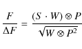
where S is the signal map, W is the weight map (the reciprocal of the noise map, squared), and P is a Gaussian of the same size as the beam. The
We generated two GMF maps, one for each iteration performed in
Minicrush (see Sect. 3.2.2). Setting a threshold
![]() ,
which
roughly corresponds to a signal-to-noise level of 4, we extracted 19
sources in the first GMF map and 22 sources in the second. We decided
to be conservative and not include in the final catalog the sources
that had appeared in the GMF map of the iterated map. In addition, we
excluded the two sources that were present in the first GMF map but
not in the second. Our final source list thus contains 17 sources.
,
which
roughly corresponds to a signal-to-noise level of 4, we extracted 19
sources in the first GMF map and 22 sources in the second. We decided
to be conservative and not include in the final catalog the sources
that had appeared in the GMF map of the iterated map. In addition, we
excluded the two sources that were present in the first GMF map but
not in the second. Our final source list thus contains 17 sources.
Figure 5 shows the GMF map calculated using the iterated signal map. The black contour indicates the 2 mJy/beam noise level, and the red circle has a diameter of 10 arcmin. The 17 identified sources are marked.
Table 2: List of sources extracted from the LABOCA map.
Whereas source finding was done in the GMF map, measurement of the properties of the identified sources was done in the signal map. The following scheme was used:
- 1.
- We searched for the peak value in the GMF map and fitted a two-dimensional Gaussian.
- 2.
- The position obtained from that fit was used as a starting guess in the fit to the real source in the signal map. The fitted function is the sum of a two-dimensional Gaussian and a tilted plane. The use of a plane reduces the effect of remaining sidelobes around bright sources. Those are due to the filtering in the data reduction and are not completely removed by the iterative method described in Sect. 3.2.2 (Fig. 3). Unless the source is clearly extended, the width of the Gaussian was fixed to that of the beam.
- 3.
- The integrated flux density of each extracted source was calculated by integrating only the Gaussian part of the fitted function.
- 4.
- The fitted Gaussian was then subtracted from the GMF map and a new search for the peak was performed.
- 5.
- We iterated over the previous steps until the peak value in the GMF map was smaller than 9. This value was inferred from the simulations described in the next section.
![\begin{figure}
\par\includegraphics[width=8.8cm,clip]{13833f5.eps}
\end{figure}](/articles/aa/full_html/2010/06/aa13833-09/img92.png)
|
Figure 5:
Gaussian filtered map, with the 17 detected sources marked with circles. The numbering of the sources is the same as in
Table 2. The black contour corresponds to the 2
mJy/beam level in the noise map and the dashed circle marks the
central 10 |
| Open with DEXTER | |
4.3 Completeness
In order to understand the systematics of the source extraction
procedure and quantify the extent to which the values of
![]() correspond to real sources, we turned to simulations. A Gaussian
source of the size of the beam was added at a random location within
the central 10
correspond to real sources, we turned to simulations. A Gaussian
source of the size of the beam was added at a random location within
the central 10![]() -diameter region of a randomly selected jackknife
map, and the Gaussian filtered map was produced, using Eq. (1). We stepped through a range of values of the flux densities of the simulated source, ranging from 1 to 15 mJy, with a
spacing of 0.5 mJy. For each flux density value, 500 sources were
simulated and placed at a random location, and the GMF maps were used
to find the simulated sources. Once they were found, a two-dimensional
circular Gaussian was fitted to the simulated signal map at the same
location. For each flux density bin, we then extracted information
about the completeness and the recovered flux as a function of the
input flux density value.
-diameter region of a randomly selected jackknife
map, and the Gaussian filtered map was produced, using Eq. (1). We stepped through a range of values of the flux densities of the simulated source, ranging from 1 to 15 mJy, with a
spacing of 0.5 mJy. For each flux density value, 500 sources were
simulated and placed at a random location, and the GMF maps were used
to find the simulated sources. Once they were found, a two-dimensional
circular Gaussian was fitted to the simulated signal map at the same
location. For each flux density bin, we then extracted information
about the completeness and the recovered flux as a function of the
input flux density value.
Figure 6 shows the results. The flux boosting is calculated as the fraction of the measured flux of a source to the input flux density. At flux densities larger than 6 mJy we see that, in the absence of confusion noise, no boosting is observed. For lower flux densities the flux boosting becomes larger than one, so that extracted sources are those that are placed on positive noise peaks, making them rise above the noise. Sources randomly placed in noise voids are not extracted.
The completeness is defined as the fraction of sources that are
recovered from the simulated maps out of the 500 input sources. We
see
that at 6 mJy the observations are 100% complete. At the level of
4.6 mJy, which is the flux of the most dim source in our sample,
the
completeness is ![]() 85%. Therefore, our sample is highly complete,
and completeness corrections are not very important.
85%. Therefore, our sample is highly complete,
and completeness corrections are not very important.
Other groups use instead the final signal map when simulating the completeness (e.g. Scott et al. 2008), but we wanted to focus our attention in these simulation on the effect of statistical noise in the map. No source confusion noise is present in the jackknife maps. In the following section, we discuss the effect of confusion noise and use noise-free sky realizations with a Schechter distribution to quantify the flux boosting for an individual source extracted from the real map.
4.4 Flux boosting due to confusion noise
Several SMG surveys have shown that the number counts steepen towards higher flux densities (e.g. Scott et al. 2006; Coppin et al. 2006). Therefore there are many more sources at low than at high flux densities. Most of those faint sources are below the noise level of submm maps, but they influence photometric measurements of extracted sources, acting as a ``sea'' of sources, often referred to as ``confusion noise''. This effect has been discussed by e.g. Condon (1974) and Hogg & Turner (1998). Recently, Coppin et al. (2005) discussed the effect of confusion noise on flux boosting in the SCUBA Groth strip survey, and used a Bayesian technique to ``deboost'' the fluxes. We employ a similar technique to estimate the amount of flux boosting for our detected sources, which we describe in Appendix A. The derived flux boosting corrections are small for most sources. The deboosted flux densities are listed in Table 2.
![\begin{figure}
\par\includegraphics[width=8cm,clip]{13833f6.eps}
\end{figure}](/articles/aa/full_html/2010/06/aa13833-09/img94.png)
|
Figure 6: Results of the Monte Carlo simulations performed to estimate the degree of completeness of the source extraction algorithm and the accuracy of the measured flux density at a given value of the input flux density. |
| Open with DEXTER | |
4.5 Lensing correction
We built a simple lensing model of the Bullet cluster in order to
estimate the magnification of our observed submm sources. The model
consists of two spherically symmetric components representing the main
component of the Bullet cluster and the subcomponent (the actual
``bullet'' to the west). Figure 7 (left) shows contours
of the projected mass distribution inferred from weak-lensing
observations by Clowe et al. (2006), overlaid on our 870 ![]() m image.
We used the fits to the weak-lensing observations made by
Bradac et al. (2006) to the masses within a certain projected radius R of each component,
m image.
We used the fits to the weak-lensing observations made by
Bradac et al. (2006) to the masses within a certain projected radius R of each component,
![]() ,
with
,
with
![]() and n=0.8 for the main cluster and
and n=0.8 for the main cluster and
![]() and n= 1.1 for the subcluster. To place
the two mass components, we used the information given in Table 2 of
the paper by Bradac et al. The redshift of our simulated Bullet cluster was set to 0.296 and that
of the source plane to z=2.5. Note that the magnification values
are not very sensitive to the redshift of the sources: varying it from
z=2 to z=3 changes the magnifications by less than 10%. The
magnification map was calculated following the derivation in the book
by Schneider et al. (1992). This numerical calculation provides results along the lines of those
obtained analytically for two point masses by
Schneider & Weiss (1986) and for two isothermal spheres by
Shin & Evans (2008), but in the case of two power-law projected mass distributions.
Because the model does not include lensing by the individual cluster
galaxies, the location of the critical lines differ from the observed
ones by about 10 arcsec. The true magnification for a given source
must therefore differ from our derived values. Nevertheless, this
simple model makes it possible to estimate the individual
magnifications and the average magnification in a certain
region. Using the calculated magnifications, we corrected the measured
flux densities. The lensing-corrected values are listed in
Table 2.
and n= 1.1 for the subcluster. To place
the two mass components, we used the information given in Table 2 of
the paper by Bradac et al. The redshift of our simulated Bullet cluster was set to 0.296 and that
of the source plane to z=2.5. Note that the magnification values
are not very sensitive to the redshift of the sources: varying it from
z=2 to z=3 changes the magnifications by less than 10%. The
magnification map was calculated following the derivation in the book
by Schneider et al. (1992). This numerical calculation provides results along the lines of those
obtained analytically for two point masses by
Schneider & Weiss (1986) and for two isothermal spheres by
Shin & Evans (2008), but in the case of two power-law projected mass distributions.
Because the model does not include lensing by the individual cluster
galaxies, the location of the critical lines differ from the observed
ones by about 10 arcsec. The true magnification for a given source
must therefore differ from our derived values. Nevertheless, this
simple model makes it possible to estimate the individual
magnifications and the average magnification in a certain
region. Using the calculated magnifications, we corrected the measured
flux densities. The lensing-corrected values are listed in
Table 2.
![\begin{figure}
\par\includegraphics[height=7.2cm,clip]{13833f7_1.eps}\includegraphics[height=7.2cm,clip]{13833f7_2.eps}
\end{figure}](/articles/aa/full_html/2010/06/aa13833-09/img98.png)
|
Figure 7: Left: signal-to-noise map with overlaid circles indicating extracted submm sources. The contours show the the projected mass density from the weak lensing analysis by Clowe et al. (2006). The contours range from 40 to 85% of the maximum value and are spaced by 15%. The weak lensing map was retrieved from the website http://flamingos.astro.ufl.edu/1e0657/public.html. The rectangles show the regions of complete coverage of Spitzer MIPS (small rectangle) and IRAC (large rectangle). Right: signal map (in units of Jy/beam) with contours of the X-ray surface brightness from XMM-Newton observations. The noise level in the signal map increases rapidly towards the outskirts because of the low coverage there. |
| Open with DEXTER | |
![\begin{figure}
\par\includegraphics[width=15.2cm]{13833f8.eps}
\end{figure}](/articles/aa/full_html/2010/06/aa13833-09/img99.png)
|
Figure 8:
1 |
| Open with DEXTER | |
5 Discussion
5.1 Searching for infrared counterparts to the submm sources
The identification of optical counterparts to SMGs is often difficult due to their optical faintness, as much of the starburst luminosity is highly obscured by dusty clouds.
Rest-frame infrared photometry of SMGs is usually possible because the
extinction is much smaller than in the optical. With the Spitzer
satellite and its imaging photometers IRAC (Fazio et al. 2004)
and MIPS (Rieke et al. 2004), it is now possible to obtain
high-resolution infrared images of these distant objects. The number
counts of sources at 3.6
![]() is high and counterpart
identification is complicated by the large positional uncertainty of
the submm source (see below). In the 24
is high and counterpart
identification is complicated by the large positional uncertainty of
the submm source (see below). In the 24
![]() band, the number
density of sources is smaller and a more secure counterpart
identification can be made, if a source can be identified.
band, the number
density of sources is smaller and a more secure counterpart
identification can be made, if a source can be identified.
Figure 8 shows cutouts of IRAC 4.5 and IRAC 8.0 and MIPS
24.0
![]() images of 16 sources detected in the
LABOCA map. Source #17 has only partial Spitzer coverage and is omitted
from this figure. The Spitzer data used in this study are described in
Sect. 2.2 and the coverage with respect to the
LABOCA map is shown in Fig. 7.
images of 16 sources detected in the
LABOCA map. Source #17 has only partial Spitzer coverage and is omitted
from this figure. The Spitzer data used in this study are described in
Sect. 2.2 and the coverage with respect to the
LABOCA map is shown in Fig. 7.
The full 1![]()
![]() 1
1![]() cutouts are only shown for reference
here. It is not necessary to search for infrared counterparts in such
a large field. The region of interest (within a certain search radius)
is the sum of the contributions from the mean pointing error of
LABOCA of
cutouts are only shown for reference
here. It is not necessary to search for infrared counterparts in such
a large field. The region of interest (within a certain search radius)
is the sum of the contributions from the mean pointing error of
LABOCA of ![]() 4
4
![]() ;
the statistical uncertainties on the fitted
positions, which are 1-2
;
the statistical uncertainties on the fitted
positions, which are 1-2
![]() ;
the systematic uncertainty due to
confusion noise,
;
the systematic uncertainty due to
confusion noise, ![]() 3-4
3-4
![]() and a possible misalignment between
the LABOCA and Spitzer maps of the order of 5
and a possible misalignment between
the LABOCA and Spitzer maps of the order of 5
![]() .
Together, this
adds up to a search radius of
.
Together, this
adds up to a search radius of ![]() 10
10
![]() .
.
Table 3 lists the coordinates of likely Spitzer
counterparts, found using the software SExtractor
(Bertin & Arnouts 1996), and their measured flux densities in the 3.6, 4.5, 5.8, 8.0, and
24 ![]() m bands. We extracted sources with six adjacent
pixels above 3.5
m bands. We extracted sources with six adjacent
pixels above 3.5![]() ,
and used an aperture of five pixels for the
photometry; applying the aperture corrections listed in the IRAC and
MIPS data handbooks. The listed uncertainties on the flux densities
are the statistical errors given by SExtractor. We estimate the
systematic uncertainties to be
,
and used an aperture of five pixels for the
photometry; applying the aperture corrections listed in the IRAC and
MIPS data handbooks. The listed uncertainties on the flux densities
are the statistical errors given by SExtractor. We estimate the
systematic uncertainties to be ![]() 10%. In the cases where a
source has been extracted in one IRAC channel and not another we list
upper limits.
10%. In the cases where a
source has been extracted in one IRAC channel and not another we list
upper limits.
We found in total 9 sources with infrared counterparts, and two where
counterpart identification is complicated by the larger number of
sources in the short wavelenght IRAC bands. For two sources we see an
excess of flux in the MIPS map, but it is not significant enough to be
extracted. Deeper MIPS imaging would therefore be useful. Deep
high-resolution radio maps could also be used to distinguish between
sources in the shorter wavelength bands. Comments about the individual
sources are presented below. The lack of infrared counterparts was to
be expected: for comparison, in the SHADES survey
Pope et al. (2006) found 21 secure Spitzer counterparts to the 35 submm sources. An important result is that the large positional
uncertainty of LABOCA (![]() 10
10
![]() for most sources) is reduced
because the pointing accuracy of Spitzer is less than 1''.
for most sources) is reduced
because the pointing accuracy of Spitzer is less than 1''.
Out of the nine sources with likely infrared counterparts, five have sufficient coverage to make it possible to investigate the shape of the mid-infrared SED. Ivison et al. (2004) suggested a diagram based on mid-infrared colors S8.0/S4.5 versus S24/S8.0. Based on the redshift tracks (the position as a function of redshift for a SED in color-color space) of typical starburst and AGN-type spectral energy distributions, such a diagram could distinguish between strong starburst SEDs and powerful AGN. A similar diagram was also used by Ivison et al. (2007) and Beelen et al. (2008), while Hainline et al. (2009) showed that its diagnostic capacity is limited. The five sources with identified counterparts in these three Spitzer bands have colors that lie in the starburst part of the diagram. This does not exclude the possibility of contributions from AGN to the dust heating, but indicates that the galaxies are starburst, rather than AGN, dominated. Infrared spectroscopic measurements could be used to investigate further the power source of those galaxies.
Table 3: Photometry of possible infrared counterparts to the LABOCA sources.
5.2 Notes on individual sources
Aside from Source #1, none of the other sources have been detected previously in the mm or submm. Our observation of Source #1 is discussed in the context of other observations. The few other sources for which complementary observations exist are discussed as well.
Source #1: with a deboosted flux density of
![]() mJy, this source is one of the brightest SMGs ever
detected around 870
mJy, this source is one of the brightest SMGs ever
detected around 870
![]() .
This is very likely because of its
proximity to a caustic line, which provides a large magnification.
From their lensing model, Gonzalez et al. (2009)
estimated that
the two brighter images of the galaxy, A and B, which are separated
by 8.6'', have a magnification of 25 and 50, whereas the
third image,
C, located 47'' away from the first one, would have a magnification
four times lower than the first one. Our final map was smoothed to
22'' and our fit to the Source #1 gives a position between the
images A and B; the flux that we measure comes most likely from
those
two images. The total magnification is therefore 75.
.
This is very likely because of its
proximity to a caustic line, which provides a large magnification.
From their lensing model, Gonzalez et al. (2009)
estimated that
the two brighter images of the galaxy, A and B, which are separated
by 8.6'', have a magnification of 25 and 50, whereas the
third image,
C, located 47'' away from the first one, would have a magnification
four times lower than the first one. Our final map was smoothed to
22'' and our fit to the Source #1 gives a position between the
images A and B; the flux that we measure comes most likely from
those
two images. The total magnification is therefore 75.
In the LABOCA study of the protocluster J2142-4423 by
Beelen et al. (2008) the brightest source has a flux density of
21.1 mJy. The flux density at 850 ![]() m, which is one of
the SCUBA wavelengths, can be extrapolated using a submm spectral
index of 2.7, giving a flux density 7% higher than at 870
m, which is one of
the SCUBA wavelengths, can be extrapolated using a submm spectral
index of 2.7, giving a flux density 7% higher than at 870 ![]() m. The SCUBA flux of Source #1 would therefore be around
51 mJy. For comparison, the brightest source in the SHADES survey
(Coppin et al. 2006) has 22 mJy (and a signal-to-noise ratio of 4.9). In the submm survey of massive clusters of galaxies,
Knudsen et al. (2008) detected two bright sources towards
Abell 478 and Abell 2204, with flux densities of 25.0 and 22.2 mJy
respectively.
m. The SCUBA flux of Source #1 would therefore be around
51 mJy. For comparison, the brightest source in the SHADES survey
(Coppin et al. 2006) has 22 mJy (and a signal-to-noise ratio of 4.9). In the submm survey of massive clusters of galaxies,
Knudsen et al. (2008) detected two bright sources towards
Abell 478 and Abell 2204, with flux densities of 25.0 and 22.2 mJy
respectively.
Source #1 was detected using the AzTEC bolometer array at
1.1 mm (W08); we can compare the astrometric position,
angular size and
integrated flux density with the values measured at 870 ![]() m.
m.
- Position: the distance between the estimated central
position of the two sources is 4.1
 .
This is well within the
pointing error margins of the two telescopes.
.
This is well within the
pointing error margins of the two telescopes.
- Source size: W08 reports a source size of
 .
To compare that with the
LABOCA source, we smoothed our map to the AzTEC resolution of
30
,
and fitted a two-dimensional Gaussian. The fitted FWHMs at
this resolution are
.
To compare that with the
LABOCA source, we smoothed our map to the AzTEC resolution of
30
,
and fitted a two-dimensional Gaussian. The fitted FWHMs at
this resolution are
 ,
in good agreement with the value of W08.
,
in good agreement with the value of W08.
- Flux density: after removal of the contribution from
the Sunyaev-Zeldovich effect, the flux density of the source at
1.1 mm was estimated to 13.5 mJy (Wilson et al. 2008). This
value, however, is too low and is being revised to about 20 mJy
(Wilson, priv. comm.), which would give a
spectral index
 between the two
measurements.
between the two
measurements.
Figure 9 shows the spectral energy distribution of
Source #1. The measured data points are from from Spitzer, BLAST,
LABOCA and AzTEC. We compared the models of
Lagache et al. (2003) of
template starburst galaxies to those data points. We used a
magnification of 75, assuming that the flux comes from
images A and B discussed by Gonzalez et al. (2009). We display the SED of a starburst galaxy at redshift 2.9, which is the redshift estimate of
Rex et al. (2009), with a total luminosity of
![]() .
The SED of a more redshifted galaxy, at redshift 3.9, with a
luminosity of
.
The SED of a more redshifted galaxy, at redshift 3.9, with a
luminosity of
![]() is in better agreement with the
long-wavelength data. However, it does not fit the 24
is in better agreement with the
long-wavelength data. However, it does not fit the 24 ![]() m value. Although we have not done a formal fit, it seems
that the current data would require a different template SED.
Alternatively, the uncertainties on the data points may have been
seriously underestimated.
m value. Although we have not done a formal fit, it seems
that the current data would require a different template SED.
Alternatively, the uncertainties on the data points may have been
seriously underestimated.
![\begin{figure}
\par\includegraphics[width=8.5cm,clip]{13833f9.eps}
\end{figure}](/articles/aa/full_html/2010/06/aa13833-09/img151.png)
|
Figure 9:
Spectral energy distribution of Source #1. The curves
show modeled SEDs of starburst galaxies taken from the templates
of Lagache et al. (2003) magnified by a factor of 75. The
magnification factor is taken from the lensing model used by
Gonzalez et al. (2009) who find a magnification of 25 for the
first image and of 50 for the second. The dotted-dashed curve
corresponds to a starburst galaxy of intrinsic total luminosity
|
| Open with DEXTER | |
We do not list any Spitzer photometry of source #1 because accurate measurement would require not only processing the raw data but also a careful subtraction of the foreground elliptical that lies between the two images of that source. Such a work has been performed by Gonzalez et al. (2009) and we used their quoted values in the analysis.
Source #2: this is our second most significant detection at
Gaussian filter value 29.9 or signal-to-noise ratio
![]() .
No
previous mm or submm detection of this source has been reported,
although in the map showing the detection of Source #1 in W08 (their
Fig. 1) there is an indication that they also detected this source.
.
No
previous mm or submm detection of this source has been reported,
although in the map showing the detection of Source #1 in W08 (their
Fig. 1) there is an indication that they also detected this source.
Figure 8 shows that this galaxy has likely counterparts in
all available Spitzer bands. There is a source to the north of the
center of the LABOCA detection in the 3.6 and 4.5 ![]() m maps that
might be the reason for the apparent elongation of the red contour
towards the north. However, this source is outside the 10
m maps that
might be the reason for the apparent elongation of the red contour
towards the north. However, this source is outside the 10
![]() search radius and does not show up in the 24
search radius and does not show up in the 24 ![]() m map.
m map.
Source #3: a bright, extended Spitzer source is seen to the
southeast of the LABOCA position. Its large angular size at 8.0 ![]() m and its distance from the submm position indicates that it
is not the infrared counterpart. It is detected in the 2MASS catalog,
but no redshift is indicated. Two sources are detected within the
10
m and its distance from the submm position indicates that it
is not the infrared counterpart. It is detected in the 2MASS catalog,
but no redshift is indicated. Two sources are detected within the
10
![]() circle. The source closest to the LABOCA position is
identified in all IRAC band, whereas the other source is only found in
IRAC1 and IRAC2. Both these sources are very faint due to this source
confusion we choose to not list a counterpart. A flux excess is
identified in the MIPS map, but it is not significant enough to be
extracted by SExtractor.
circle. The source closest to the LABOCA position is
identified in all IRAC band, whereas the other source is only found in
IRAC1 and IRAC2. Both these sources are very faint due to this source
confusion we choose to not list a counterpart. A flux excess is
identified in the MIPS map, but it is not significant enough to be
extracted by SExtractor.
Source #4: the identification of a counterpart to the submm
source is complicated by the bright foreground source seen in all five
Spitzer bands. This source, at z=0.097, is also found in the 2MASS
catalog. In radio observations with the ATCA array,
Liang et al. (2000) detected a source at the position of the
foreground galaxy. The flux density at 1.344 GHz is
![]() mJy
and drops towards higher frequencies. The source is not detected at
4.4 and 8.8 GHz.
mJy
and drops towards higher frequencies. The source is not detected at
4.4 and 8.8 GHz.
Due to the positional offset, it is not very likely that the submm
emission seen in the LABOCA map is caused by the z=0.097 galaxy south
of the submm detection. There is a possibility that a small part of
the total LABOCA flux density is coming from this foreground source, but
not a substantial fraction. A faint source is detected to the north of
the central position, but its position is slightly outside the
10
![]() search radius.
search radius.
Source #5:
two sources with detections in the IRAC 1, 2 and 4 bands are found
close to the central position. A MIPS detection is associated with the
centralmost source, which is situated only 1
![]() from the
LABOCA position. The other source lies 6
from the
LABOCA position. The other source lies 6
![]() away which point towards
a counterpart association with the central source. High resolution
radio imaging is needed to completely differentiate between these two
sources, but we list the most central source here as a
counterpart. Another source, to the south-east, is detected only in
IRAC1, and is likely too faint to be a counterpart.
away which point towards
a counterpart association with the central source. High resolution
radio imaging is needed to completely differentiate between these two
sources, but we list the most central source here as a
counterpart. Another source, to the south-east, is detected only in
IRAC1, and is likely too faint to be a counterpart.
Source #6: a source is detected in the IRAC 1 and 2 bands south of the LABOCA position. The brighter source north-west of the central position is further out than the search radius.
Source #7: a significant source is detected in the IRAC 1, 2 and 3 bands west of the center of this source. Its SED is declining towards the longer wavelength IRAC bands.
Source #8: a counterpart is identified in all Spitzer bands to the north of the LABOCA central position.
Source #9: almost 10
![]() from the central position lies a
significant source, which is probably too far out and too bright to be
the SMG counterpart. Closer to the central position two IRAC1 sources
are extracted, but their similar flux levels and distance to the
center makes the counterpart association ambiguous. We therefore
choose to not list a counterpart for this SMG.
from the central position lies a
significant source, which is probably too far out and too bright to be
the SMG counterpart. Closer to the central position two IRAC1 sources
are extracted, but their similar flux levels and distance to the
center makes the counterpart association ambiguous. We therefore
choose to not list a counterpart for this SMG.
Source #10: a bright MIPS source with counterparts in IRAC 1, 2 and 3 is situated close to the LABOCA central position. This is a tentative counterpart to the LABOCA source.
Source #11: a possible counterpart is detected in all the Spitzer bands.
Source #15: the source to the northeast is identified as a counterpart and exists in all the Spitzer bands.
Source #17: lies outside the R=5' circle from the center
in a region when the noise is high. Our deboosting algorithm failed in
that case, so we only quote the measured flux density of
![]() mJy. This very bright source is also present in the
AzTEC 1.1 mm map (Hughes & Aretxaga, priv. comm.).
mJy. This very bright source is also present in the
AzTEC 1.1 mm map (Hughes & Aretxaga, priv. comm.).
![\begin{figure}
\par\includegraphics[width=8.8cm,clip]{13833f10.eps}
\end{figure}](/articles/aa/full_html/2010/06/aa13833-09/img154.png)
|
Figure 10:
Cumulative number counts derived from the central 10 arcmin of the 870 |
| Open with DEXTER | |
5.3 Number counts
Figure 10 shows the cumulative number counts, defined as the number density of sources with flux density larger than S, denoted N(>S), derived from our observations and from other studies. There is good overall agreement between our results and those from previous LABOCA and SCUBA surveys, although our surveyed area is not as large as that of other studies, as reflected by the larger errorbars.
Because of the gravitational magnification, the surveyed area in the source plane is smaller than that in the image plane. We used the simple lensing model described in Sect. 4.5 to calculate the mean magnification in the central part of the map used for the analysis. We calculated a mean magnification factor of 3.3, i.e. the area of the source plane is 3.3 times smaller than the surveyed area in the image plane. The magnification of the source fluxes is also taken into account by using the de-magnified source flux densities listed in Table 2.
Our counts were inferred from the 13 sources found within the central
10 arcmin (the region within the red circle shown in Fig. 5), where the noise is uniform. From our 13 sources we
construct the number counts in four flux-bins. We probe the counts
down to ![]() 0.64 mJy, a regime which can be investigated only by
utilizing foreground lensing clusters. The number of points per
flux-bin and the counts are displayed in Table 4. We
estimate errorbars for each data point from Poissonian statistics,
using the tabulated values from Gehrels (1986).
0.64 mJy, a regime which can be investigated only by
utilizing foreground lensing clusters. The number of points per
flux-bin and the counts are displayed in Table 4. We
estimate errorbars for each data point from Poissonian statistics,
using the tabulated values from Gehrels (1986).
In Fig. 10 we also show the results from the LESS survey
(filled diamonds), which covered an area of
![]() of the Extended Chandra Deep Field South to a uniform noise
level of 1.2 mJy/beam (Weiß et al. 2009).
That survey has a
noise level comparable to ours, but it covers an area which is
10 times larger. The apparent deficit of galaxies in the LESS has
also
been demonstrated in other wavebands (see Weiß et al. 2009 and
references therein). The results of the LABOCA study of the
protocluster J2142-4423 at z=2.38 (Beelen et al. 2008) are
plotted in Fig. 10 as open circles. The excess seen at
S>3 mJy might be an effect of clustering of submm sources in the
protocluster.
of the Extended Chandra Deep Field South to a uniform noise
level of 1.2 mJy/beam (Weiß et al. 2009).
That survey has a
noise level comparable to ours, but it covers an area which is
10 times larger. The apparent deficit of galaxies in the LESS has
also
been demonstrated in other wavebands (see Weiß et al. 2009 and
references therein). The results of the LABOCA study of the
protocluster J2142-4423 at z=2.38 (Beelen et al. 2008) are
plotted in Fig. 10 as open circles. The excess seen at
S>3 mJy might be an effect of clustering of submm sources in the
protocluster.
We also compare with the SCUBA surveys from Coppin et al. (2006) (SHADES, filled circles) and Knudsen et al. (2008) (open boxes). The SHADES survey, which covered blank fields, probes the high-end of the number counts, while the Knudsen et al. survey targeted 10 lensing galaxy clusters and reached lower flux levels. Although our surveyed area is similar to that of Knudsen et al. (2008), we find only one sub-mJy source compared to the seven found by Knudsen et al. This is because their survey covers a larger area of high magnification.
Table 4: Cumulative number counts based on the central 10 arcminutes of our map.
5.4 Resolving the cosmic infrared background
It is interesting to investigate how much of the cosmic infrared background (CIB) flux is resolved in our LABOCA observation. The CIB was discovered by the COBE instruments FIRAS and DIRBE (Hauser et al. 1998; Fixsen et al. 1998). Those experiments detected an isotropic infrared background signal that was thought to originate from the integrated effect of star formation in the history of the universe (Dwek et al. 1998). But the coarse resolution of the COBE satellite made it impossible to resolve the sources responsible for the background signal. The detection of those sources had to wait for the invention of mm and submm bolometer cameras on large ground-based telescopes, resulting in angular resolutions of tens of arcseconds.
Because of the steep number counts, most of the flux coming from submm galaxies originates in low-flux sources. Therefore, observations of lensing foreground clusters that probe the faintest number counts potentially will resolve a large fraction of the CIB.
We use the central region of 10![]() diameter for this
calculation. The amount of CIB flux in that area, at 870
diameter for this
calculation. The amount of CIB flux in that area, at 870 ![]() m is
estimated from Eq. (1) of Dwek et al. (1998) and yields
m is
estimated from Eq. (1) of Dwek et al. (1998) and yields ![]() 900 mJy. The total flux in the sources extracted from the LABOCA map within
that region (the same sources that are used for the number counts, but
without the flux correction due to magnification) is
900 mJy. The total flux in the sources extracted from the LABOCA map within
that region (the same sources that are used for the number counts, but
without the flux correction due to magnification) is
![]() mJy. This calculation is valid because gravitational lensing preserves
surface brightness. Thus, 14% of the CIB has been resolved in the
LABOCA observations.
mJy. This calculation is valid because gravitational lensing preserves
surface brightness. Thus, 14% of the CIB has been resolved in the
LABOCA observations.
5.5 Residual SZ emission
Although the data have been filtered to remove the extended emission, some level of residual SZ emission may be present. Close inspection of the central region of the map shows extended emission between the two brighter sources, Source #1 and #2. We note that W08 (their Fig. 1) see a similar extended structure around the same central sources. In order to set an upper limit to the amount of residual SZ signal present in the region of the map covered by the Bullet cluster (which corresponds roughly to the area of a disk with an outer radius of about 2 arcmin), we calculated the difference between the excess flux density in that region (estimated from Fig. 4) and the flux density in resolved point sources in the same region. Removing the positive noise contribution estimated from the jackknife noise maps we find that 40 mJy residual SZ emission might be present in the final map.
We can use the results of the APEX-SZ observations of the decrement at
150 GHz by Halverson et al. (2009)
to estimate the SZ flux density across the sky area covered by the
Bullet cluster. Halverson et al. (2009) fitted an elliptical beta
model using an X-ray prior on
![]() and found
a core radius
and found
a core radius
![]() ,
an axial ratio of
,
an axial ratio of
![]() and a central Compton parameter
and a central Compton parameter
![]() .
Integrating the beta model over the central region with a maximum
radius of 2 arcmin, and taking for simplicity a spherical model
with the corresponding core radius, we estimate that the total SZ flux
density from that area is of the order of 400 mJy. Therefore, we
cannot exclude that a maximum of 10% of the total SZ flux of the
Bullet cluster may remain in the map in the form of extended emission.
.
Integrating the beta model over the central region with a maximum
radius of 2 arcmin, and taking for simplicity a spherical model
with the corresponding core radius, we estimate that the total SZ flux
density from that area is of the order of 400 mJy. Therefore, we
cannot exclude that a maximum of 10% of the total SZ flux of the
Bullet cluster may remain in the map in the form of extended emission.
6 Conclusions
Continuum observations at 870 ![]() m of the Bullet cluster have been
presented. The data were filtered to remove large-scale signal such as
the Sunyaev-Zeldovich increment from the cluster. The main results are summarized below:
m of the Bullet cluster have been
presented. The data were filtered to remove large-scale signal such as
the Sunyaev-Zeldovich increment from the cluster. The main results are summarized below:
- Seventeen submm sources with signal-to-noise ratios larger than 4 were detected in the map. Their measured fluxes densities range from 4.6 to 48 mJy. For each source but one, which lies in a noisy area, we calculated the value of the flux density corrected for the flux boosting due to confusion noise and for the gravitational magnification by the cluster.
- The brightest submm source coincides with a previously reported
galaxy at an estimated redshift of 2.7-2.9 detected by Spitzer and
the AzTEC and BLAST experiments. With its flux density of 48 mJy it
is one of the brightest submm galaxy ever
detected. After correction for gravitational magnification
 ,
the intrinsic flux of the source is about
,
the intrinsic flux of the source is about
 mJy.
mJy.
- We found reliable infrared counterparts for nine of the submm sources. An infrared color-color analysis suggests that they have starburst-dominated spectral energy distributions.
- The cumulative number counts derived from the observations agree well with those from other surveys.
- The observations resolve 14% of the cosmic infrared background
radiation at 870
 m, in a sky area of
  78.5 arcmin2.
We thank the APEX staff for excellent support during the observations. C.H. and D.J. thank the Swedish Research Council for financial support. M.S., K.B., and F.B. acknowledge support from a grant within the DFG Priority Program 1177. H.Q. acknowledges partial support from the FONDAP Centro de Astrofísica. We thank Alexandre Beelen, John H. Black, David Hughes and Itziar Aretxaga for stimulating discussions, and Florian Pacaud for providing us with the XMM map of the Bullet cluster shown as contours in Fig. 7. We are grateful to Attila Kovács for writing Minicrush and being helpful to us during the data reduction. We thank the referee for a careful reading of the manuscript and useful comments.This work is based in part on observations made with the Spitzer Space Telescope, which is operated by the Jet Propulsion Laboratory, California Institute of Technology under a contract with NASA.
Appendix A: Flux deboosting
This appendix describes the flux deboosting algorithm used in this work, following the prescription in Scott et al. (2008, Sect. 5.1), whose notation we use in the rest of this section.
![\begin{figure}
\par\includegraphics[width=17.7cm,clip]{13833fA1.eps}
\end{figure}](/articles/aa/full_html/2010/06/aa13833-09/img168.png)
|
Figure A.1: Solid curves: posterior flux distributions for measured flux densities of 3, 5 and 7 mJy and a noise level of 1.2 mJy. Dashed curves: measured flux distributions, modelled as Gaussian functions. Dotted-dashed curve: prior flux density distributions estimated from noise-free simulations, populating maps with a Schechter flux distribution (Eq. (A.3)). The prior (red dotted-dashed) is identical in all three panels. The posterior flux distribution is the result of multiplying the blue dashed curve by the red dot-dashed curve and normalizing. The two vertical lines in each panel show the measured flux (rightmost line) and the maximum of the posterior flux distribution (leftmost line). The difference between the two lines indicates the amount of flux boosting. |
| Open with DEXTER | |
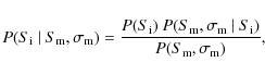
where
The likelihood of observing the data,
![]() ,
is modeled by a Gaussian distribution. This is valid because of the
Gaussian distribution of pixel values in the jackknife maps (see
Fig. 4). The likelihood is
,
is modeled by a Gaussian distribution. This is valid because of the
Gaussian distribution of pixel values in the jackknife maps (see
Fig. 4). The likelihood is
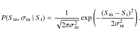
We calculated the prior sky distribution
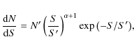
as fitted to the source counts in the SCUBA SHADES survey of Coppin et al. (2006). We used
We generated ![]() 106 sky maps and measured the pixel distribution
in each of them. The mean distribution of pixel values in these maps
is a measure of
106 sky maps and measured the pixel distribution
in each of them. The mean distribution of pixel values in these maps
is a measure of
![]() .
.
From those simulated sky maps, we could calculate the posterior flux
distribution of a source extracted from the map with flux density
![]() and uncertainty
and uncertainty
![]() :
it is obtained by multiplying the
prior
:
it is obtained by multiplying the
prior
![]() (from the simulations) with the Gaussian distribution
(Eq. (A.2)), and dividing by
(from the simulations) with the Gaussian distribution
(Eq. (A.2)), and dividing by
![]() .
.
Figure A.1 shows examples of posterior flux distributions
for three combinations of ![]() and
and
![]() .
The amount of flux
boosting for a certain source depends both on the signal-to-noise
ratio and the value of the flux density; for example, for a
signal-to-noise ratio of 4, a source with a measured flux density of
10 mJy will have been boosted more than a source with a flux density
of 5 mJy.
.
The amount of flux
boosting for a certain source depends both on the signal-to-noise
ratio and the value of the flux density; for example, for a
signal-to-noise ratio of 4, a source with a measured flux density of
10 mJy will have been boosted more than a source with a flux density
of 5 mJy.
References
- Andreani, P., Böhringer, H., dall'Oglio, G., et al. 1999, ApJ, 513, 23 [NASA ADS] [CrossRef] [Google Scholar]
- Austermann, J. E., Dunlop, J. S., Perera, T. A., et al. 2010, MNRAS, 401, 160, 4 [NASA ADS] [CrossRef] [Google Scholar]
- Beelen, A., Omont, A., Bavouzet, N., et al. 2008, A&A, 485, 645 [NASA ADS] [CrossRef] [EDP Sciences] [Google Scholar]
- Bertin, E., & Arnouts, S. 1996, A&AS, 117, 393 [NASA ADS] [CrossRef] [EDP Sciences] [Google Scholar]
- Bertoldi, F., Carilli, C., Aravena, M., et al. 2007, ApJS, 172, 132 [NASA ADS] [CrossRef] [Google Scholar]
- Blain, A. W. 1997, MNRAS, 290, 553 [NASA ADS] [Google Scholar]
- Blain, A. W. 1998, MNRAS, 297, 502 [NASA ADS] [CrossRef] [Google Scholar]
- Blain, A. W., & Longair, M. S. 1993, MNRAS, 264, 509 [NASA ADS] [CrossRef] [Google Scholar]
- Blain, A. W., Smail, I., Ivison, R. J., Kneib, J.-P., & Frayer, D. T. 2002, Phys. Rep., 369, 111 [NASA ADS] [CrossRef] [Google Scholar]
- Borys, C., Chapman, S., Halpern, M., et al. 2003, MNRAS, 344, 385 [NASA ADS] [CrossRef] [Google Scholar]
- Bradac, M., Clowe, D., Gonzalez, A. H., et al. 2006, ApJ, 652, 937 [NASA ADS] [CrossRef] [Google Scholar]
- Chapman, S. C., Scott, D., Borys, C., et al. 2002, MNRAS, 330, 92 [NASA ADS] [CrossRef] [Google Scholar]
- Clowe, D., Bradac, M., Gonzalez, A. H., et al. 2006, ApJ, 648, L109 [NASA ADS] [CrossRef] [Google Scholar]
- Condon, J. J. 1974, ApJ, 188, 279 [NASA ADS] [CrossRef] [Google Scholar]
- Coppin, K., Halpern, M., Scott, D., Borys, C., & Chapman, S. 2005, MNRAS, 357, 1022 [NASA ADS] [CrossRef] [Google Scholar]
- Coppin, K., Chapin, E. L., Mortier, A. M. J., et al. 2006, MNRAS, 372, 1621 [NASA ADS] [CrossRef] [Google Scholar]
- Cowie, L. L., Barger, A. J., & Kneib, J.-P. 2002, AJ, 123, 2197 [NASA ADS] [CrossRef] [Google Scholar]
- Dwek, E., Arendt, R. G., Hauser, M. G., et al. 1998, ApJ, 508, 106 [NASA ADS] [CrossRef] [Google Scholar]
- Fazio, G. G., Hora, J. L., Allen, L. E., et al. 2004, ApJS, 154, 10 [NASA ADS] [CrossRef] [Google Scholar]
- Fixsen, D. J., Dwek, E., Mather, J. C., Bennett, C. L., & Shafer, R. A. 1998, ApJ, 508, 123 [NASA ADS] [CrossRef] [Google Scholar]
- Gehrels, N. 1986, ApJ, 303, 336 [NASA ADS] [CrossRef] [Google Scholar]
- Gomez, P., Romer, A. K., Peterson, J. B., et al. 2004, in Plasmas in the Laboratory and in the Universe: New Insights and New Challenges, ed. G. Bertin, D. Farina, & R. Pozzoli, AIP Conf. Proc., 703, 361 [Google Scholar]
- Gonzalez, A. H., Clowe, D., Bradac, M., et al. 2009, ApJ, 691, 525 [NASA ADS] [CrossRef] [Google Scholar]
- Güsten, R., Nyman, L. Å., Schilke, P., et al. 2006, A&A, 454, L13 [NASA ADS] [CrossRef] [EDP Sciences] [Google Scholar]
- Hainline, L. J., Blain, A. W., Smail, I., et al. 2009, ApJ, 699, 1610 [NASA ADS] [CrossRef] [Google Scholar]
- Halverson, N. W., Lanting, T., Ade, P. A. R., et al. 2009, ApJ, 701, 42 [NASA ADS] [CrossRef] [Google Scholar]
- Hauser, M. G., Arendt, R. G., Kelsall, T., et al. 1998, ApJ, 508, 25 [NASA ADS] [CrossRef] [Google Scholar]
- Hincks, A. D., Acquaviva, V., Ade, P., et al. 2009, [arXiv:0907.0461] [Google Scholar]
- Hogg, D. W., & Turner, E. L. 1998, PASP, 110, 727 [NASA ADS] [CrossRef] [Google Scholar]
- Ivison, R. J., Greve, T. R., Serjeant, S., et al. 2004, ApJS, 154, 124 [NASA ADS] [CrossRef] [Google Scholar]
- Ivison, R. J., Greve, T. R., Dunlop, J. S., et al. 2007, MNRAS, 380, 199 [Google Scholar]
- Knudsen, K. K., van der Werf, P. P., & Kneib, J.-P. 2008, MNRAS, 384, 1611 [NASA ADS] [CrossRef] [Google Scholar]
- Kovács, A. 2008, in SPIE Conf., 7020 [Google Scholar]
- Lagache, G., Dole, H., & Puget, J. 2003, MNRAS, 338, 555 [NASA ADS] [CrossRef] [Google Scholar]
- Liang, H., Hunstead, R. W., Birkinshaw, M., et al. 2000, ApJ, 544, 686 [NASA ADS] [CrossRef] [Google Scholar]
- Loeb, A., & Refregier, A. 1997, ApJ, 476, L59+ [Google Scholar]
- Markevitch, M., Gonzalez, A. H., David, L., et al. 2002, ApJ, 567, L27 [NASA ADS] [CrossRef] [Google Scholar]
- Nord, M., Basu, K., Pacaud, F., et al. 2009, A&A, 506, 623 [NASA ADS] [CrossRef] [EDP Sciences] [Google Scholar]
- Plagge, T., Benson, B. A., Ade, P. A. R., et al. 2009, [arXiv:0911.2444] [Google Scholar]
- Pope, A., Scott, D., Dickinson, M., et al. 2006, MNRAS, 370, 1185 [NASA ADS] [CrossRef] [Google Scholar]
- Rex, M., Ade, P. A. R., Aretxaga, I., et al. 2009, ApJ, 703, 348 [NASA ADS] [CrossRef] [Google Scholar]
- Rieke, G. H., Young, E. T., Engelbracht, C. W., et al. 2004, ApJS, 154, 25 [NASA ADS] [CrossRef] [Google Scholar]
- Sanders, D. B., & Mirabel, I. F. 1996, ARA&A, 34, 749 [NASA ADS] [CrossRef] [Google Scholar]
- Schechter, P. 1976, ApJ, 203, 297 [Google Scholar]
- Schneider, P., & Weiss, A. 1986, A&A, 164, 237 [NASA ADS] [Google Scholar]
- Schneider, P., Ehlers, J., & Falco, E. E. 1992, Gravitational Lenses, ed. E. J. F. E. E. Schneider, P. [Google Scholar]
- Scott, S. E., Dunlop, J. S., & Serjeant, S. 2006, MNRAS, 370, 1057 [NASA ADS] [CrossRef] [Google Scholar]
- Scott, K. S., Austermann, J. E., Perera, T. A., et al. 2008, MNRAS, 385, 2225 [NASA ADS] [CrossRef] [Google Scholar]
- Serjeant, S., Dunlop, J. S., Mann, R. G., et al. 2003, MNRAS, 344, 887 [NASA ADS] [CrossRef] [Google Scholar]
- Shin, E. M., & Evans, N. W. 2008, MNRAS, 390, 505 [NASA ADS] [Google Scholar]
- Siringo, G., Kreysa, E., Kovács, A., et al. 2009, A&A, 497, 945 [NASA ADS] [CrossRef] [EDP Sciences] [Google Scholar]
- Smail, I., Ivison, R. J., & Blain, A. W. 1997, ApJ, 490, L5+ [NASA ADS] [CrossRef] [Google Scholar]
- Smail, I., Ivison, R. J., Blain, A. W., et al. 1998, ApJ, 507, L21 [NASA ADS] [CrossRef] [Google Scholar]
- Smail, I., Ivison, R. J., Owen, F. N., Blain, A. W., & Kneib, J.-P. 2000, ApJ, 528, 612 [NASA ADS] [CrossRef] [Google Scholar]
- Springel, V., & Farrar, G. R. 2007, MNRAS, 380, 911 [NASA ADS] [CrossRef] [Google Scholar]
- Weiß, A., Kovács, A., Coppin, K., et al. 2009, ApJ, 707, 1201 [NASA ADS] [CrossRef] [Google Scholar]
- Wilson, G. W., Hughes, D. H., Aretxaga, I., et al. 2008, MNRAS, 390, 1061 [NASA ADS] [CrossRef] [Google Scholar]
Footnotes
- ... observations
![[*]](/icons/foot_motif.png)
- Swedish program ID O-079.F-9304A and ESO program ID E-380.A-3036A.
- ... telescope
- This publication is based on data acquired with the Atacama Pathfinder EXperiment (APEX). APEX is a collaboration between the Max-Planck-Institut für Radioastronomie, the European Southern Observatory, and Onsala Space Observatory.
- ...
Tool''
- http://ssc.spitzer.caltech.edu/tools/senspet/
- ...
Minicrush
- Minicrush can be downloaded from http://www.submm.caltech.edu/sharc/crush/download.htm.
- ...BoA
- BoA can be downloaded from http://www.apex-telescope.org/bolometer/laboca/boa/.
All Tables
Table 1: Properties of the Spitzer data used in this study.
Table 2: List of sources extracted from the LABOCA map.
Table 3: Photometry of possible infrared counterparts to the LABOCA sources.
Table 4: Cumulative number counts based on the central 10 arcminutes of our map.
All Figures
|
|
Figure 1:
Left: layout of the bolometers on the
LABOCA array. Each circle represents one bolometer that was active
at the time of the observations. The two rectangles illustrate the
sizes of the two raster+spiral scanning pattern for one bolometer
(solid line-small pattern, dashed line-large
pattern). Right: movement pattern for one bolometer during
the large scanning pattern. This pattern has a
|
| Open with DEXTER | |
| In the text | |
|
|
Figure 2:
Color image of the 870 |
| Open with DEXTER | |
| In the text | |
|
|
Figure 3:
Radial profiles of the brightest source (source #1): in
the first iteration of the data reduction (solid line and boxes),
a source model was successively built during the data reduction;
in the second iteration (dashed line + circles), a
4.5 |
| Open with DEXTER | |
| In the text | |
|
|
Figure 4: Solid curve: histogram of the pixel distribution in the central 10 arcmin of the signal-to-noise map. Dashed curve: histogram of the mean pixel distribution in the same region of the jackknife maps, as described in the text. The jackknife procedure has removed the excess positive signal (due to the sources) and the negative signal (due to the sidelobes) that are present in the signal map. |
| Open with DEXTER | |
| In the text | |
|
|
Figure 5:
Gaussian filtered map, with the 17 detected sources marked with circles. The numbering of the sources is the same as in
Table 2. The black contour corresponds to the 2
mJy/beam level in the noise map and the dashed circle marks the
central 10 |
| Open with DEXTER | |
| In the text | |
|
|
Figure 6: Results of the Monte Carlo simulations performed to estimate the degree of completeness of the source extraction algorithm and the accuracy of the measured flux density at a given value of the input flux density. |
| Open with DEXTER | |
| In the text | |
|
|
Figure 7: Left: signal-to-noise map with overlaid circles indicating extracted submm sources. The contours show the the projected mass density from the weak lensing analysis by Clowe et al. (2006). The contours range from 40 to 85% of the maximum value and are spaced by 15%. The weak lensing map was retrieved from the website http://flamingos.astro.ufl.edu/1e0657/public.html. The rectangles show the regions of complete coverage of Spitzer MIPS (small rectangle) and IRAC (large rectangle). Right: signal map (in units of Jy/beam) with contours of the X-ray surface brightness from XMM-Newton observations. The noise level in the signal map increases rapidly towards the outskirts because of the low coverage there. |
| Open with DEXTER | |
| In the text | |
|
|
Figure 8:
1 |
| Open with DEXTER | |
| In the text | |
|
|
Figure 9:
Spectral energy distribution of Source #1. The curves
show modeled SEDs of starburst galaxies taken from the templates
of Lagache et al. (2003) magnified by a factor of 75. The
magnification factor is taken from the lensing model used by
Gonzalez et al. (2009) who find a magnification of 25 for the
first image and of 50 for the second. The dotted-dashed curve
corresponds to a starburst galaxy of intrinsic total luminosity
|
| Open with DEXTER | |
| In the text | |
|
|
Figure 10:
Cumulative number counts derived from the central 10 arcmin of the 870 |
| Open with DEXTER | |
| In the text | |
|
|
Figure A.1: Solid curves: posterior flux distributions for measured flux densities of 3, 5 and 7 mJy and a noise level of 1.2 mJy. Dashed curves: measured flux distributions, modelled as Gaussian functions. Dotted-dashed curve: prior flux density distributions estimated from noise-free simulations, populating maps with a Schechter flux distribution (Eq. (A.3)). The prior (red dotted-dashed) is identical in all three panels. The posterior flux distribution is the result of multiplying the blue dashed curve by the red dot-dashed curve and normalizing. The two vertical lines in each panel show the measured flux (rightmost line) and the maximum of the posterior flux distribution (leftmost line). The difference between the two lines indicates the amount of flux boosting. |
| Open with DEXTER | |
| In the text | |
Copyright ESO 2010
Current usage metrics show cumulative count of Article Views (full-text article views including HTML views, PDF and ePub downloads, according to the available data) and Abstracts Views on Vision4Press platform.
Data correspond to usage on the plateform after 2015. The current usage metrics is available 48-96 hours after online publication and is updated daily on week days.
Initial download of the metrics may take a while.