Bandwidth in bolometric interferometry

R. Charlassier; E. F. Bunn; J.-Ch. Hamilton; J. Kaplan; S. Malu

doi:10.1051/0004-6361/200913446

Home

All issues

Volume 514 (May 2010)

A&A, 514 (2010) A37

Full HTML

Free Access

Issue		A&A Volume 514, May 2010


Article Number		A37
Number of page(s)		13
Section		Astronomical instrumentation
DOI		https://doi.org/10.1051/0004-6361/200913446
Published online		07 May 2010

A&A 514, A37 (2010)

Bandwidth in bolometric interferometry

R. Charlassier¹ - E. F. Bunn² - J.-Ch. Hamilton¹ - J. Kaplan¹ - S. Malu³

1 - APC, Université Denis Diderot-Paris 7, CNRS/IN2P3, CEA, Observatoire de Paris, 10 rue A. Domon and L. Duquet, Paris, France
2 - Physics Department, University of Richmond, Richmond, VA 23173, USA
3 - Inter-University Centre for Astronomy and Astrophysics (IUCAA), Pune 411 007, India

Received 9 October 2009 / Accepted 13 January 2010

Abstract
Context. Bolometric interferometry is a promising new technology with potential applications to the detection of B-mode polarization fluctuations of the cosmic microwave background (CMB). A bolometric interferometer will have to take advantage of the wide spectral detection band of its bolometers to be competitive with imaging experiments. A crucial concern is that interferometers are assumed to be significantly affected by a spoiling effect known as bandwidth smearing.
Aims. We investigate how the bandwidth modifies the work principle of a bolometric interferometer and affects its sensitivity to the CMB angular power spectra.
Methods. We obtain analytical expressions for the broadband visibilities measured by broadband heterodyne and bolometric interferometers. We investigate how the visibilities must be reconstructed in a broadband bolometric interferometer and show that this critically depends on hardware properties of the modulation phase shifters. If the phase shifters produce shifts that are constant with respect to frequency, the instrument works like its monochromatic version (the modulation matrix is not modified), while if they vary (linearly or otherwise) with respect to frequency, one has to perform a special reconstruction scheme, which allows the visibilities to be reconstructed in frequency subbands. Using an angular power spectrum estimator that accounts for the bandwidth, we finally calculate the sensitivity of a broadband bolometric interferometer. A numerical simulation is performed that confirms the analytical results.
Results. We conclude that (i) broadband bolometric interferometers allow broadband visibilities to be reconstructed regardless of the type of phase shifters used and (ii) for dedicated B-mode bolometric interferometers, the sensitivity loss caused by bandwidth smearing is quite acceptable, even for wideband instruments (a factor of 2 loss for a typical 20% bandwidth experiment).

Key words: instrumentation: interferometers - polarization - cosmic microwave background - submillimeter: diffuse background - cosmology: observations

1 Introduction

The detection of B-mode polarization anisotropies in the cosmic microwave background (CMB) is one of the most exciting challenges of modern cosmology. The weakness of the expected signal requires the development of highly sensitive experiments with an exquisite control of systematic errors. Most experiments or projects dedicated to this quest are based on well-known direct imaging technology. An appealing alternative called bolometric interferometry has been proposed (Tucker et al. 2003). This technology combines the advantages of interferometry in handling systematic effects and those of bolometric detectors in enhancing sensitivity. The two teams that accepted the challenge (Charlassier & the BRAIN coll. 2008; Timbie et al. 2006) have combined their efforts to form the QUBIC collaboration (Kaplan & the QUBIC coll. 2009).

In (Charlassier et al. 2009), hereafter (C09), we introduced a simple formalism for the general design of a bolometric interferometer operating at a monochromatic frequency and showed that its phase shifting scheme must respect a property which we called ``coherent summation of equivalent baselines''. This scheme was optimized further in (Hyland et al. 2009). In (Hamilton et al. 2008), hereafter (H08), we calculated the sensitivity of a bolometric interferometer and showed that this technology can be competitive with imaging experiments and heterodyne interferometers for the measurement of CMB B-mode. For the sake of simplicity, we did not deal with the question of bandwidth in (C09) and (H08).

We know that a dedicated B-mode bolometric interferometer will have to use the wide spectral detection band of its bolometers to be competitive with imaging experiments. On the other hand, the bandwidth is often considered as a crucial issue in radio-interferometry; if the raw sensitivity of radio interferometer detectors increases as the square root of the bandwidth, there is a secondary effect, well known as bandwidth smearing, which can largely degrade the global sensitivity. When the signals originating in a point source interfere after being collected by two broadband receivers, the resulting fringe pattern is smeared by an envelope whose amplitude depends on the bandwidth, consequently leading to a degradation in the signal-to-noise ratio - see for instance (Thompson et al. 2001). We later see that these two main characteristics remain in bolometric interferometry: the bolometers' sensitivity also increases as the square root of the bandwidth, and a bandwidth smearing of the observables, the visibilities, degrades the global sensitivity of the instrument (however, because the observation of CMB angular correlations requires a poorer spatial resolution than the observation of point sources to which classical radio-interferometers are mostly dedicated, this smearing will lead to a less critical sensitivity loss). But we also see that an additional kind of bandwidth issue occurs, because in bolometric interferometry, visibilities are not measured directly but by solving a linear problem.

We investigate how the visibilities are smeared in heterodyne and bolometric interferometers with wide spectral bands and large primary beams in Sect. 2. We investigate how the work principle of bolometric interferometry is affected by bandwidth in Sect. 3. We show in particular that the visibilities can be reconstructed exactly as in the monochromatic case detailed in (C09) if the modulation phase shifts are constant with respect to frequency, while one has to perform the special reconstruction scheme described in Sect. 4 when the modulation phase shifts vary with respect to frequency. In Sect. 5, we introduce an angular power spectrum estimator that accounts for the bandwidth and estimate how the bandwidth smearing results in a degradation of the sensitivity for B-mode experiments. A numerical simulation that confirms our analytical results is presented in Sect. 6.

2 Visibilities measured by generic interferometers with wide spectral bands and large primary beams

2.1 Monochromatic visibilities

The observables measured by a monochomatic interferometer working at a frequency $\nu _0$ and looking at a radiation field of spectral power $I_{\nu}(\vec{n})$ , in units of [ ${\rm W~Hz^{-1}~sr^{-1}}$ ], are called the visibilities. A monochromatic visibility is defined for one baseline $\vec{u}_{0}$ , which is the vector separation between two horns in units of the electromagnetic wavelength of the radiation. Its expression is given by

$\begin{displaymath}V_{I}^{\nu_{0}}(\vec{u}_{0})=\int I_{\nu_{0}}(\vec{n})A_{\nu_... ...{n})\ {\rm exp}(i2\pi\vec{u}_{0}\cdot\vec{n})\ {\rm d}\vec{n}, \end{displaymath}$

(1)

where $A_{\nu}(\vec{n})=B_{\nu}^{2}(\vec{n})$ is the square of the beam of the input horns (assumed to be identical), conventionally normalized to one at its maximum. Here we can make a first important observation about the understanding of bandwidth in interferometry: a monochromatic visibility defined by a pair of horns separated by a distance $\vec{d}_{0}$ and working at frequency $\nu _0$ is the same observable as a monochromatic visibility defined by another pair of horns separated by a distance $\vec{d}=\vec{d}_{0}\frac{\nu_{0}}{\nu}$ and working at frequency $\nu$ . The two visibilities indeed match the baseline $\vec{u}_{0}=\vec{d}_{0}\frac{\nu_{0}}{c}$ . This property, sometimes called the equivalence theorem of interferometry, is actually true only if the two pairs of horns have the same beam (meaning that their surfaces are necessarily different) and if the observed radiation field $S(\vec{n})$ has the same spatial variations at both frequencies (this is of course true in the case of CMB observations).

2.2 Broadband visibilities for a generic interferometer

We consider now an interferometer that is sensitive to a finite spectral band through a bandpass function $J(\nu-\nu_0)$ , centered at frequency $\nu _0$ . We arbitrarily define the bandwidth $\Delta\nu$ of the instrument as

$\begin{displaymath}\Delta\nu=\frac{1}{J(0)}\int J(\nu-\nu_0){\rm d}\nu. \end{displaymath}$

(2)

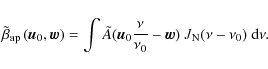
We define a generic interferometer to be an instrument in which visibilities are directly given by the outputs of the detectors (this is the case in heterodyne interferometry, but not in bolometric interferometry). The expression for a broadband visibility measured by a generic interferometer - in power units, for a baseline $\vec{u}_{0}=\vec{d}_{0}\frac{\nu_{0}}{c}$ - is then

$\begin{displaymath}V_{I}^{\Delta\nu}(\vec{u}_{0})=\iint I_{\nu}(\vec{n})A_{\nu}(... ...ac{\nu}{c}\right)\ J(\nu-\nu_{0})\ {\rm d}\nu\ {\rm d}\vec{n}. \end{displaymath}$

(3)

The baselines define a plane usually called the uv-plane. It is better to write the visibility as a convolution in the uv-plane to understand the bandwidth effect,

$\displaystyle V_{I}^{\Delta\nu}(\vec{u}_{0})$	=	$\displaystyle \iiiint\tilde{I}_{\nu}(\vec{w})\tilde{A}_{\nu}(\vec{w'})J(\nu-\nu_{0})$
		$\displaystyle \times{\rm e}^{{\rm i}2\pi(\frac{\nu}{\nu_{0}}\vec{u}_{0}-\vec{w}-\vec{w'}) \cdot\vec{n}}{\rm d}\vec{w}{\rm d}\vec{w'}{\rm d}\vec{n}{\rm d}\nu,$	(4)

where we have introduced the Fourier transform of the signal and that of the beam (w is the associated transform variable), i.e.,

$\begin{displaymath}I_{\nu}(\vec{n})=\int\tilde{I}_{\nu}(\vec{w})\exp(-{\rm i}2\pi\vec{w}\cdot\vec{n}){\rm d}\vec{w} \end{displaymath}$

(5)

$\begin{displaymath}A_{\nu}(\vec{n})=\int\tilde{A}_{\nu}(\vec{w'})\exp(-{\rm i}2\pi\vec{w'}\cdot \vec{n}){\rm d}\vec{w'}. \end{displaymath}$

(6)

In the flat-sky approximation, the integral over the field $\vec{n}$ gives a delta function, and the expression of the broadband visibility is finally

$\begin{displaymath}V_{I}^{\Delta\nu}(\vec{u}_{0})=J(0)\ \Delta\nu\int\tilde{I}_{... ...}(\vec{w})\tilde{\beta}(\vec{u}_{0},\vec{w})\ {\rm d}\vec{w}, \end{displaymath}$

(7)

where we have defined the convolution kernel in the uv-plane

$\begin{displaymath}\tilde{\beta}(\vec{u}_{0},\vec{w})=\int\frac{\tilde{I}_{\nu}(... ...}{\nu_{0}}-\vec{w}\right)\ J_{\rm N}(\nu-\nu_{0})\ {\rm d}\nu, \end{displaymath}$

(8)

in which we have introduced the normalized bandpass function $J_{\rm N}(\nu-\nu_0)=J(\nu-\nu_0)/\Delta\nu$ . The convolution kernel (which depends on $\vec{u}_{0}$ ) contains the entire effect of the bandwidth smearing. For a monochromatic visibility, the convolution kernel in the uv-plane is just the Fourier transform of the beam $\tilde{A}(\vec{w})$ .

In the following, to allow for complete analytic calculation, we first ignore the frequency dependence of both the signal and the beam. We write

$\begin{displaymath}\tilde{A}(\vec{w})=\tilde{A}_{\nu_{0}}(\vec{w})\approx\tilde{... ...)=\tilde{I}_{\nu_{0}}(\vec{w})\approx\tilde{I}_{\nu}(\vec{w}). \end{displaymath}$

(9)

This defines the approximate form of the convolution kernel

$\begin{displaymath}\tilde{\beta}_{\rm ap}\left(\vec{u}_{0},\vec{w}\right)=\int\t... ...ac{\nu}{\nu_{0}}-\vec{w})\ J_{\rm N}(\nu-\nu_{0})\ {\rm d}\nu. \end{displaymath}$

(10)

This approximation allows us to obtain an intuitive idea of how the bandwidth smearing acts with good enough accuracy to estimate the sensitivity loss. We discuss in Sect. 2.5 a refined form of the kernel that takes into account the frequency dependence of the beam and the intensity. As shown in Fig. 2, the difference between the approximate kernel, derived in Sect. 2.3, and the refined kernel is small.

$\begin{figure} \par\includegraphics[width=8cm,clip]{13446fig01.ps}\hspace*{4mm}\includegraphics[width=8cm,clip]{13446fig02.ps} \end{figure}$

Figure 1:

Left: convolution kernel in the uv-plane for a monochromatic interferometer, which is actually just the Fourier transform of the primary beam, for a 90 GHz central frequency and a Gaussian beam with $15^{\circ }$ FWHM. Right: approximate convolution kernel in the uv-plane for a baseline $\vec{u}_{0}$ (matching $l\sim 100$ ), for a 20% bandwidth interferometer, for a Gaussian bandpass function centered at 90 GHz and a Gaussian beam with $15^{\circ }$ FWHM.

Open with DEXTER

2.3 Approximate analytical form of the kernel

In order to perform the analytical calculation, we also assume a Gaussian normalized bandpass function

$\begin{displaymath}J_{\rm N}(\nu-\nu_0)=\frac{1}{\sigma_{\nu}\sqrt{2\pi}}\exp\left(-\frac{(\nu-\nu_0)^{2}}{2\sigma_{\nu}^{2}}\right)\cdot \end{displaymath}$

(11)

The instrument bandwidth is related to the standard deviation of the Gaussian distribution by $\Delta\nu=\sigma_{\nu}\sqrt{2\pi}$ . We assume a Gaussian beam for the horns, with the usual convention A(0)=1, leading to the following beam in the uv-plane

$\begin{displaymath}\tilde{A}(\vec{w})=\Omega\exp(-\pi\Omega\vec{w}^{2}). \end{displaymath}$

(12)

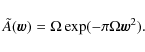
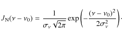
As previously explained, we ignore the frequency dependence of the beam. The integral of the beam over the sky is defined for the central frequency, $\Omega=\Omega_{\nu_{0}}$ . The expression of the kernel is then

$\displaystyle \tilde{\beta}_{\rm ap}(\vec{u}_{0},\vec{w})=\frac{\Omega}{\sigma_... ...{w}\right)^{2}-\frac{(\nu-\nu_{0})^{2}}{2\sigma_{\nu}^{2}}\right]}\ {\rm d}\nu.$

(13)

This can be analytically integrated (details are given in Appendix A) and written in the form

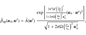
$\begin{displaymath}\tilde{\beta}_{\rm ap}(\vec{u}_{0},\vec{w'})=\tilde{A}(\vec{w... ...left(\frac{\sigma_{\nu}}{\nu_{0}}\right)^{2}\vec{u}_{0}^{2}}}, \end{displaymath}$

(14)

where we have made the variable substitution

$\begin{displaymath}\vec{w'}=\vec{u}_{0}-\vec{w}. \end{displaymath}$

(15)

We can define the effective beam in real space for a broadband interferometer $\Omega_{\rm s}$ as the value at $\vec{w'}={0}$ of the Fourier transform of the kernel

$\begin{displaymath}\Omega_{\rm s}=\tilde{\beta}_{\rm ap}(\vec{u}_{0},{0})=\frac{\Omega}{\kappa_{1}}, \end{displaymath}$

(16)

with

$\begin{displaymath}\kappa_{1}=\sqrt{1+2\pi\Omega\left(\frac{\sigma_{\nu}}{\nu_{0}}\right)^{2}\vec{u}_{0}^{2}}, (\kappa_{1}\geq1). \end{displaymath}$

(17)

We can finally rewrite the kernel as

$\displaystyle \tilde{\beta}_{\rm ap}(\vec{u}_{0},\vec{w'})$	=	$\displaystyle \tilde{A}(\vec{w'})\times\frac{1}{\kappa_{1}}\times\exp\left[2\pi... ...nu}}{\nu_{0}}\right)^{2}\Omega_{\rm s}^{2}(\vec{u}_{0}\cdot\vec{w'})^{2}\right]$	(18)
	=	$\displaystyle \tilde{A}(\vec{w'})\times\frac{1}{\kappa_{1}}\times\exp\left[\pi\... ...}^{2}}\right)\frac{(\vec{u}_{0}\cdot\vec{w'})^{2}}{\vec{u}_{0}^{2}}\right]\cdot$	(19)

This $\kappa _{1}$ factor is an indicator of the importance of bandwidth smearing. It reaches its minimal value 1 for a monochromatic interferometer. One immediately sees that interferometers with ``small'' primary beams and/or ``small'' baselines are less affected by the bandwidth smearing (see Fig. 4). We compare the convolution kernels of monochromatic and broadband interferometers in Fig. 1. One can clearly see that the effect of the bandwidth smearing is to stretch the kernel, in the baseline direction only, by which the Fourier transform of the signal is convolved. When $\kappa _{1}$ is close to 1 (i.e., $\left(\frac{\sigma_{\nu}}{\nu_{0}}\right)^{2}\vec{u}_{0}^{2}\ll\frac{1}{2\pi\Omega}$ ), the size of the ``bandwidth part'' of the kernel is smaller than the ``beam part'' and thus the signal is not degraded by the bandwidth: this is quite intuitive since a signal already convolved by a kernel of width $\sigma_{a}$ is not significantly degraded if it is convolved again by a kernel of width $\sigma_{b}$ such as $\sigma_{b}<\sigma_{a}$ . The physical interpretation in real space is that the bandwidth smearing makes the beam narrower, by a factor $\kappa _{1}$ that depends on the baseline length: for a given multipole l, the fraction of sky observed by a broadband interferometer is actually $f_{\rm sky}^{\Delta_{\nu}}(l)=f_{\rm sky}(l)/\kappa_{1}$ (cf. Sect. 5).

$\begin{figure} \par\includegraphics[width=8cm,clip]{13446fig03.ps}\hspace*{4mm}\includegraphics[width=8cm,clip]{13446fig04.ps} \end{figure}$

Figure 2:

Left: the black full line shows longitudinal profile of the kernel for monochromatic visibilities, while the color lines show the longitudinal profile of the convolution kernel for baselines corresponding to l₀=50, 100, 200, for an instrument with a 20% Gaussian bandwidth centered at 90 GHz and $15^{\circ }$ FWHM horns. Approximate kernel: full coloured line. Refined kernel numerically computed: dotted coloured line. Kernel for monochromatic visibilities: black full line. Right: same but with a top hat shaped bandwidth.

Open with DEXTER

2.4 Broadband visibilities in temperature units for CMB experiments

It is more convenient to work with visibilities in temperature units when studying CMB temperature and polarization anisotropies. If $B_{\nu}$ is the intensity of the observed field, in units of [ ${\rm W~Hz^{-1}~m^{-2}~sr^{-1}}$ ], the spectral power collected by a horn of surface S is

$\begin{displaymath}I_{\nu}=SB_{\nu}. \end{displaymath}$

(20)

CMB experiments observe small spatial fluctuations over the sky

$\begin{displaymath}I_{\nu}(\vec{n})=I_{\nu}+\Delta I_{\nu}(\vec{n}). \end{displaymath}$

(21)

The oscillating term of the visibilities washes out the constant part of the spectral power, so the visibilities can be rewritten

$\begin{displaymath}V_{I}^{\Delta\nu}(\vec{u}_{0})\!=\!\!\iint\Delta I_{\nu}(\vec... ...\frac{\nu}{c}) J(\nu-\nu_{0}\right){\rm d}\nu~ {\rm d}\vec{n}. \end{displaymath}$

(22)

The temperature fluctuations over the sky are linked to the power fluctuations by

$\begin{displaymath}\Delta I_{\nu}(\vec{n})=\frac{\partial I_{\nu}}{\partial T}\D... ...vec{n})=S\frac{\partial B_{\nu}}{\partial T}\Delta T(\vec{n}). \end{displaymath}$

(23)

We can then define the broadband visibilities in temperature units as

$\begin{displaymath}V_{T}^{\Delta\nu}(\vec{u}_{0})[{\rm in\ K]}=\frac{V_{I}^{\Del... ...left.(\partial B_{\nu}/\partial T)\right\vert _{\nu_{0}}}\cdot \end{displaymath}$

(24)

Following the same arguments as previously, one can show that

$\begin{displaymath}V_{T}^{\Delta\nu}(\vec{u}_{0})=\Delta\nu\int\tilde{\Delta T}(\vec{w})\tilde{\beta}^{T}(\vec{u}_{0},\vec{w})\ {\rm d}\vec{w}, \end{displaymath}$

(25)

where we have introduced the Fourier transform of the temperature field,

$\begin{displaymath}\Delta T(\vec{n})=\int\tilde{\Delta T}(\vec{w})\exp(-i2\pi\vec{w}\cdot \vec{n}){\rm d}\vec{w}, \end{displaymath}$

(26)

and a temperature convolution kernel,

$\begin{displaymath}\tilde{\beta}^{T}(\vec{u}_{0},\vec{w})=\int\left( \frac{ \par... ...}{\nu_{0}}-\vec{w}\right)\ J_{\rm N}(\nu-\nu_{0})\ {\rm d}\nu. \end{displaymath}$

(27)

If we neglect the dependence of both the signal and the beam on frequency, this kernel actually becomes the one defined in Eq. (10),

$\begin{displaymath}\tilde{\beta}_{\rm ap}^{T}(\vec{u}_{0},\vec{w})\rightarrow\tilde{\beta}_{\rm ap}(\vec{u}_{0},\vec{w}).\end{displaymath}$

(28)

$\begin{figure} \par\includegraphics[width=8cm,clip]{13446fig05.ps}\hspace*{4mm}\includegraphics[width=8cm,clip]{13446fig06.ps} \end{figure}$	Figure 3: Left: shift of the effective l window function as a function of l₀, dashed lines for a Gaussian bandwidth, solid lines for a top hat one. Right: the variation in $\kappa _{1}$ as a function of l₀, dashed lines for a Gaussian bandwidth, solid lines for a top hat one.
Open with DEXTER

$\begin{figure} \par\includegraphics[width=8cm,clip]{13446fig07.ps}\hspace*{4mm} \includegraphics[width=8cm,clip]{13446fig08.ps} \end{figure}$

Figure 4:

Left: sensitivity degradation on C_lextraction due to bandwidth smearing for multipoles between 50 and 200; the quantity $K_{\rm sp}$ is plotted for a dedicated B-mode bolometric interferometer with a 15-degree FWHM primary beam, for, respectively $\Delta \nu / \nu _0 = 10$ , 20, and 30% bandwidth. Right: the quantity $(0.20/ \Delta \nu ) \times K_{\rm sp}(l)$ , showing the competition between smearing and broadening, is plotted as a function of bandwidth for l=100, for the same B-mode bolometric interferometer.

Open with DEXTER

2.5 A refined kernel

The intensity $B_{\nu}$ of the observed field actually depends on frequency for a black body source at temperature T such that

$\begin{displaymath}B_{\nu}=\frac{2h\nu^{3}}{c^{2}}\frac{1}{\exp\left({h\nu}/{k_{\rm B}T}\right)-1}\cdot \end{displaymath}$

(29)

Inside the bandwidth, the frequency dependence of the T derivative of $B_{\nu}$ is approximated well by a power law

$\begin{displaymath}\frac{\partial B_{\nu}}{\partial T}\simeq\left.\frac{\partial... ...0}}/{k_{\rm B}T}}+1}{{\rm e}^{{h\nu_{0}}/{k_{\rm B}T}}-1}\cdot \end{displaymath}$

(30)

The beam of the horns also depends on frequency. The surface of the horns S, the solid angle covered $\Omega$ , and the frequency of observation $\nu$ are related by $S\Omega=\kappa\frac{c^{2}}{\nu^{2}}$ , leading to $\Omega_{\nu}=\Omega_{\nu_{0}}\frac{\nu_{0}^{2}}{\nu^{2}}$ . This frequency dependence of a Gaussian beam can be modeled by modifying its Fourier transform as

$\begin{displaymath}\tilde{A_{\nu}}(\vec{w})=\Omega\frac{\nu_{0}^{2}}{\nu^{2}}\exp\left(-\pi\Omega\frac{\nu_{0}^{2}}{\nu^{2}}\vec{w}^{2}\right). \end{displaymath}$

(31)

Figure 2 shows for several values of lhow the approximate kernel of Eq. (19) is refined when one takes into account the above frequency dependences of the beam and the intensity. The signal and the beam dependencies largely compensate each other, and the difference between the two kernels turns out to be negligible considering the accuracy level required for the sensitivity loss estimation. The main difference is a shift in the centroid of the window function shown in the left panel of Fig. 3, which is absent in the approximate kernel. This will introduce systematics that have to be corrected for. We also show what happens for a more realistic top-hat-shaped bandwidth (right panel of Fig. 2, solid lines in Fig. 3). For the data extraction of a given instrument, the convolution kernel has to be computed numerically; however, the approximate Gaussian kernel provides a good enough accuracy to estimate the sensitivity loss. In the remainder of this paper, we use the approximate analytical form of the kernel, and write $\tilde{\beta}$ instead of $\tilde{\beta}_{\rm ap}$ . Finally, the right panel of Fig. 3 shows the variation in $\kappa _{1}$ with l₀ for a Gaussian (dashed line) and a top hat (solid line) bandwidth.

3 Visibilities measured by broadband bolometric interferometers

The effect of the bandwidth is more subtle in a bolometric interferometer than in a generic interferometer, because the visibilities are not measured directly. As described in (C09), a time-domain modulation of the visibilities is performed by controlled phase shifters - located behind each polarization channel (twice the number of horns)- which take some well-chosen time-sequences of discrete phase values. The corresponding time-sequences of bolometers' measurements will allow us to recover, independently for each bolometer, all the different visibilities, by solving a linear problem of the form $S=A \cdot X$ , where X is a vector including the visibilities, S is a vector including a time-sequence of one bolometer's measurements, and A is a coefficient matrix depending on the phase shift sequences. In the following, we generalize the (C09) formalism, taking the bandwidth into account. As in the generic case, we assume in this section that the detectors (here the bolometers) are sensitive to a spectral bandwidth $\Delta\nu$ , by means of a bandpass function $J(\nu-\nu_0)$ centered on the frequency $\nu _0$ .

3.1 Signal in broadband bolometers

We consider a bolometric interferometer consisting of $N_{\rm h}$ horns, whose beams are defined by the same function $B(\vec{n})$ and $N_{\rm out}$ bolometers. The electric field at the output of polarization splitters, corresponding to horn i coming from direction $\vec{n}$ for polarization $\eta \ (\Vert {\rm\ or \ } \bot)$ is

$\begin{displaymath}\epsilon_{i,\eta}(\vec{n}) = B(\vec{n}) E_{i,\eta}(\vec{n}). \end{displaymath}$

(32)

During a time sample k, each controlled phase shifter adds to its associated input channel the phase $\Phi^k_{i,\eta}(\nu)$ . After combining, the electric field in one output channel is then

$\begin{displaymath}z_k(\vec{n}) = \int {z_k^\nu(\vec{n})} J(\nu-\nu_0) {\rm d}\nu, \end{displaymath}$

(33)

where

$\begin{displaymath}z_{k}^\nu(\vec{n})=\frac{1}{\sqrt{N_{{\rm out}}}}\sum_{i=0}^{... ...0}^{1}\epsilon_{i,\eta}(\vec{n})\exp[i\Phi^k_{i, \eta}(\nu)]. \end{displaymath}$

(34)

The power originating in each of the combiner outputs is averaged on timescales given by the time constant of the detector, which is much larger than the EM wave period. The power collected by a given bolometer during a time sample k is then

$\begin{displaymath}S_k=\left\langle\left\vert \iint{z^{\nu}_k(\vec{n}) J(\nu-\nu... ...}\nu {\rm d}\vec{n}} \ \right\vert^2 \right\rangle_{\rm time}. \end{displaymath}$

(35)

Signals coming from different directions of the sky are incoherent, as are signals at different frequencies, so their time-averaged correlations vanish to produce

$\begin{displaymath}\langle z_{k}^{\nu}(\vec{n})z_{k}^{\nu^{\prime} \star}(\vec{n... ...delta(\vec{n}-\vec{n}^{\prime}) \ \delta(\nu - \nu^{\prime}). \end{displaymath}$

(36)

The signal on the bolometer is finally

$\begin{displaymath}S_k = \iint{ \vert z^{\nu}_k(\vec{n}) \vert ^2 J(\nu - \nu_0) {\rm d}\nu {\rm d}\vec{n} }. \end{displaymath}$

(37)

Developing this expression leads to autocorrelation terms for each input channel and cross-correlation terms between all the possible pairs

$\begin{displaymath}S_k = S_k^{\rm auto} + S_k^{\rm cross}. \end{displaymath}$

(38)

As in the general case, one can write the visibilities as a convolution in the uv-plane, where we define $b=\{i,j\}$ , $p=\{\eta_1, \eta_2\}$ , and

$\begin{displaymath}S_{k}^{\rm cross} = \frac{2 J(0) \ \Delta \nu}{N_{\rm out}} {... ...ta}^{\rm BI}_{b,p}(\vec{u_b}, \vec{w}) {\rm d}\vec{w} \right]. \end{displaymath}$

(39)

We have defined the Fourier transform of the physical signal to be

$\begin{displaymath}\tilde{I}_{b,p}(\vec{w}) = \int E_{i, \eta_1}(\vec{n})E^\star_{j,\eta_2}(\vec{n}) \exp(i2\pi\vec{n}.\vec{w}) {\rm d}\vec{n} , \end{displaymath}$

(40)

and the kernel $\tilde{\eta}^{\rm BI}_{b,p}(\vec{u_b}, \vec{w})$ containing the phase modulation used to recover the visibilities to be

$\displaystyle \tilde{\eta}^{\rm BI}_{b,p}(\vec{u_b}, \vec{w})$	=	$\displaystyle \int \tilde{A}\left(\frac{\nu}{\nu_0} \vec{u_b} - \vec{w}\right) \! J_N(\nu-\nu_0) \! \exp[i\Delta \Phi^ k_{b,p}(\nu)] \ {\rm d}\nu,$	(41)
$\displaystyle \Delta \Phi^k_{b,p}(\nu)$	=	$\displaystyle \Phi^k_{i,\eta_1}(\nu) - \Phi^k_{j, \eta_2}(\nu),$	(42)

where $A(\vec{n})=B^2(\vec{n})$ defined the square of the beam of the input horns.

3.2 Phase shifters constant with respect to frequency

We first consider the simplest case where the phase shift values do not depend on the frequency $\nu$ . When $\Delta \Phi^k_{b,p}(\nu) = \Delta \Phi^k_{b,p}(\nu_0)$ , the phase shift term comes outside the integral over $\nu$

$\begin{displaymath}\tilde{\eta}^{\rm BI}_{b,p}(\vec{u_b}, \vec{w}) = \tilde{\beta}(\vec{u_b}, \vec{w}) \exp[i\Delta \Phi^k_{b,p}(\nu_0)]. \end{displaymath}$

(43)

The signal of the cross-correlations on the bolometer is thus the one expressed in (C09), with the broadband visibilities defined in Eq. (24) instead of the monochromatic ones

$\displaystyle S_{k}^{\rm cross} = \frac{2}{N_{\rm out}} {\rm Re}\big[ \sum_{i<j... ...m e}^{{\rm i}\Delta \Phi^k_{b,p}(\nu_0)} V^{\Delta_\nu}_{b,p}(\vec{u_b}) \big].$

(44)

Following (C09), we can introduce the broadband Stokes visibilities

$\begin{displaymath}V^{\Delta_\nu}_{S}(\vec{u_b}) = J(0) \ \Delta \nu \int \tilde{S}(\vec{w}) \tilde{\beta}(\vec{u}_b, \vec{w}) \ {\rm d}\vec{w}, \end{displaymath}$

(45)

where S stands for the Stokes parameters I, Q, U or V and $\tilde{S}$ represents their Fourier transform, and rewrite Eq. (44) as a linear combination of the Stokes visibilities defined for different baselines

$\displaystyle S_{k}^{\rm cross} = \sum_{\beta=0}^{N_{\neq}-1} \Gamma_{k, \beta} \cdot \mathsf{V}^{\Delta_\nu}_{\beta}$

(46)

where $\Gamma_{k, \beta}$ is the vector, defined in (C09), encoding the phase shifting values, and $\mathsf{V}^{\Delta_\nu}_{\beta}$ is a vector including the real and imaginary parts of the broadband Stokes visibilities. If the phase shift values of a broadband bolometric interferometer are constant with respect to frequency, the visibilities should thus be reconstructed exactly as explained in (C09), by solving a linear problem. In this case, a broadband bolometric interferometer therefore works exactly as a monochromatic one, except that the output observables will be broadband visibilities instead of monochromatic ones.

$\begin{figure} \par\includegraphics[width=8cm,clip]{13446fig09.ps}\hspace*{4mm}\includegraphics[width=8cm,clip]{13446fig10.ps} \end{figure}$

Figure 5:

Left: reconstructed temperature and polarization power spectra for a monochromatic (black squares) and a $20\%$ broadband (blue squares) bolometric interferometer (16 horns with 15 degrees FWHM primary beam, phase shifters constant with respect to frequency, 12 modulation phase shift values, no instrumental noise and $N_{\rm maps}=100$ in each case). Red lines show the input theoretical spectra. Right: relative error in the reconstruction $(\hat{C}^{\rm MC}_l-C_l)/C_l$ (squares for temperature spectra, triangles for polarization ones, black for monochromatic, blue for broadband). The green and yellow lines shows the expected error levels $1 / \sqrt {N_{\rm maps}}$ at one and two standard deviations.

Open with DEXTER

3.3 Phase shifters linear with respect to frequency

We now consider the more complicated case where the modulation phase shifters vary linearly with respect to frequency,

$\begin{displaymath}\Delta \Phi^k_{b,p}(\nu) = \Delta \Phi^k_{b,p}(\nu_0) \times \frac{\nu}{\nu_0}\cdot \end{displaymath}$

(47)

From a technological point of view, this may seem more natural, since it is automatically respected if for instance the phase shifters are just constituted by delay-lines.

For the sake of simplicity, we write $\Delta\Phi^k_{b,p}$ instead of $\Delta\Phi^k_{b,p}(\nu_0)$ in the following. As in Sect. 2, to carry out the analytical calculation, we assume both the beam and the intensity to be independent of frequency, and we assume a normalized Gaussian bandpass function J_N. We show in Appendix B that $\tilde{\eta}^{\rm BI}_{b,p}$ is then

$\displaystyle \tilde{\eta}^{\rm BI}_{b,p}(\vec{u}_b, \vec{w}) = \tilde{\beta}(\... ...{b,p}^{k})^2 G + i \Delta\Phi^k_{b,p} \left(1 \ - \ H(\vec{w})\right) \right]},$

(48)

where we have defined

G	=	$\displaystyle \left(\frac{\sigma_\nu}{\nu_0}\right)^2 \times \frac{1}{2\kappa_1^2},$	(49)
$\displaystyle H(\vec{w})$	=	$\displaystyle \left(1 - \frac{1}{\kappa_1^2}\right) \times \frac{\vec{u}_b \cdot (\vec{u}_b-\vec{w})}{\vec{u}_b^2}\cdot$	(50)

Thus the cross-correlation part of the bolometer signal can be written

$\displaystyle S_{k}^{\rm cross} = \frac{2}{N_{\rm out}} {\rm Re}\big[ \sum_{i<j... ...\ +\ {\rm i}\Delta \Phi^k_{b,p}} \ V^{LD, k, \Delta_\nu}_{b,p}(\vec{u}_b) \big]$

(51)

where we have introduced some ``phase-dependent'' broadband visibilities

$\begin{displaymath}V^{{\rm LD}, k, \Delta_\nu}_{b,p}(\vec{u}_b) = J(0) \ \Delta ... ...lde{\beta}_{b,p}^{LD, k}(\vec{u}_b, \vec{w}) \ {\rm d}\vec{w}. \end{displaymath}$

(52)

The new kernel is linked to the generic one by a rotation in the complex plane

$\begin{displaymath}\tilde{\beta}^{{\rm LD}, k}_{b,p}(\vec{u}_b, \vec{w}) = \tild... ... \vec{w}) \exp \left[-i \Delta\Phi^k_{b,p} H(\vec{w}) \right]. \end{displaymath}$

(53)

This complex factor unfortunately depends on the phase differences: this means that the definition of every visibility will slightly change between two different samples k and k'! This is of course a defect that will corrupt the linear problem.

We will show in a paper in preparation that an error varying with the modulation will lead to a dramatic leakage from the intensity visibilities into the polarization ones (which are at least two orders of magnitudes smaller in CMB observations). This prediction (which is not trivial and is not proven analytically in this article) is supported by our Monte-Carlo simulation (cf. Sect. 6): introduction of the $\eta$ -kernel of Eq. (48) in the simulation leads to a huge error on the reconstructed polarization spectrum (typically two orders of magnitude bigger than the one on temperature spectrum), as shown in Fig. 5, when the modulation matrix used to solve the problem is the monochromatic one defined in (C09). Fortunately, there is a way to get rid of this leakage, as described in Sect. 4, by reconstructing the I visibilities in sub-bands. Using the extended modulation matrix introduced in Sect. 4.3, this dramatic error source can be put under control, and the broadband polarization visibilities can be reconstructed without loss of sensitivity.

3.4 Geometrical phase shifts

In the quasi-optical combiner design considered for the QUBIC experiment (Kaplan & the QUBIC coll. 2009), some geometrical phase shifts $\Psi^k_{b,p}(\nu)$ are automatically introduced by the combiner. These phase shifts, stemming from path differences between rays in the optical combiner, vary linearly with respect to frequency:

$\begin{displaymath}\Delta \Psi^k_{b,p}(\nu) = \Delta \Psi^k_{b,p}(\nu_0) \times \frac{\nu}{\nu_0}\cdot \end{displaymath}$

(54)

But as explained in (C09), these geometrical phase shifts ought not to be used to modulate the visibilities. This means that they will not vary between the different time samples used in a reconstruction:

$\begin{displaymath}\forall k, k', \ \ \ \Delta \Psi^k_{b,p}(\nu) = \Delta \Psi^{k'}_{b,p}(\nu) \equiv \Delta \Psi_{b,p}(\nu). \end{displaymath}$

(55)

Hence they do not cause any error during the reconstruction: the $\beta$ -kernels of each different visibility are rotated in the complex plane by the same factor independent the sample. The visibilities are then measured by applying a rotation

$\displaystyle V^{{\rm GLD}, \Delta_\nu}_{b,p}(\vec{u}_b)$	=	$\displaystyle J(0) \ \Delta \nu \int \tilde{I}_{b,p}(\vec{w}) \tilde{\beta}(\vec{u}_b, \vec{w})$
		$\displaystyle \times\exp \left[-i \Delta\Psi_{b,p} H(\vec{w}) \right] \ {\rm d}\vec{w}.$	(56)

3.5 Photon noise error in reconstructed visibilities

We assume here that the modulation matrix used to reconstruct the visibilities is the monochromatic one defined in (C09); this is completely true in the case of frequency-independent phase shifters, and true for the rows concerning the polarization visibilities in the case of frequency-dependent phase shifters (see Sect. 4.3). We have shown in (C09) that the visibility covariance matrix is, where the factor $1/[J(0)\ \Delta \nu]^2$ is caused by the difference in the definitions of the monochromatic and broadband visibilities,

$\begin{displaymath}N=\frac{\sigma_0^2 N_{\rm h}}{\left[J(0) \ \Delta \nu \right]^2 \ N_{\rm out}} \times \left( A^{\rm t} \cdot A \right)^ {-1}, \end{displaymath}$

(57)

where A is a matrix including the $\Gamma_{k, \beta}$ vectors and $\sigma_0$ represents the photon noise (in watts) that would be seen by one bolometer illuminated by one horn during the time of one sample of the phase sequence. The off-diagonal elements become zero because the angles are uncorrelated from one channel to another, while the diagonal elements average to the variance in the elements in A, which equals 1 multiplied by the number of different data samples $N_{\rm d}$ . If the coherent summation of equivalent baselines scheme is adopted, the variance in the reconstructed visibilities is

$\begin{displaymath}\sigma_{V}[{\rm in \ W}] = \frac{\sqrt{N_{\rm h}}}{N_{\rm eq}... ...sigma_0}{\sqrt{N_{\rm t}}} \times \frac{1}{J(0) \ \Delta \nu}, \end{displaymath}$

(58)

where $N_{\rm t}=N_{\rm d} \times N_{\rm out}$ is the total number of time samples. We derive from Eq. (58) in Appendix E the noise in a visibility measured during a time t by a bolometric interferometer experiment, knowing the noise equivalent temperature (NET) of its bolometers, in Kelvin units,

$\begin{displaymath}\sigma_{V}[{\rm in \ K}] = \frac{\sqrt{N_{\rm h}}}{N_{\rm eq}} \frac{{\rm NET} \ \Omega}{\sqrt{t}}\cdot \end{displaymath}$

(59)

4 Virtual reconstruction sub-bands in bolometric interferometry

We show that the linear dependence in frequency of the modulation phase shifts $\Phi^k_{b,p}(\nu)$ enables independent reconstruction of the visibilities in narrower frequency subbands. This idea was first proposed by (Malu 2007). We initially interpretted this method as a way of reducing the smearing because the sub-band visibilities that are reconstructed are less smeared than the broadband ones. However we now demonstrate that its application produces a loss in signal-to-noise ratio that thwarts the gain in sensitivity, and thus makes this method inefficient for decreasing bandwidth smearing. However, as we see, this method can be succesfully set up to remove the dramatic effect described in Sect. 3.3, and thus saves the frequency-dependent option for the modulation phase shifters.

4.1 Principle

Before doing the visibility reconstruction, one can choose a number $n_{\rm vsb}$ of virtual reconstruction sub-bands of width $\delta\nu=\Delta\nu/n_{\rm vsb}$ . We emphasize that this division into subbands is purely virtual in that the hardware design does not depend on it. The $\tilde{\eta}$ -kernel becomes

$\begin{displaymath}\tilde{\eta}^{{\rm BI}, \Delta\nu}_{b,p}(\vec{u}_b, \vec{w}) ... ...{\eta}^{{\rm BI}, \delta\nu}_{b,p}[\vec{u}_b, \vec{w}, \nu_m], \end{displaymath}$

(60)

where $\tilde{\eta}^{{\rm BI}, \delta\nu}_{b,p}$ are defined as the sub-bands kernels

$\displaystyle \tilde{\eta}^{{\rm BI}, \delta\nu}_{b,p}[\vec{u}_b, \vec{w}, \nu_m]$	=	$\displaystyle \int \tilde{A}(\frac{\nu}{\nu_0} \vec{u}_b - \vec{w}) \ J_N^{\delta\nu}(\nu-\nu_m)$
		$\displaystyle \times \exp \left[i\Delta \Phi^k_{b,p}(\nu)\right] \ {\rm d}\nu,$	(61)

where $J_N^{\delta\nu}(\nu-\nu_m)$ is a bandpass function of width $\delta\nu$ centered on $\nu_m$ . The cross-correlation term is then

$\begin{displaymath}S_{k}^{\rm cross} = \frac{2}{N_{\rm out}} {\rm Re}\left[ \sum... ...i^k_{b,p} \right] V^{\delta\nu}_{b,p}(\vec{u_{b,m}}) \right], \end{displaymath}$

(62)

where we have defined

$\begin{displaymath}\Delta\Phi_{b,p,m} = \Delta\Phi_{b,p}(\nu_0) \times \frac{\nu... ...\ \ \vec{u}_{b,m} = \vec{u}_b \times \frac{\nu_m}{\nu_0}\cdot \end{displaymath}$

(63)

The sub-band visibilities $V^{\delta\nu}_{b,p}(\vec{u}_{b,m})$ are the broadband visibilities defined in the previous sections but for a $\delta\nu$ bandwidth. For each pair of horns, the $n_{\rm vsb}$ sub-bands visibilities are defined for $n_{\rm vsb}$ different baselines $\{u_{b,m}\}_{m=1,..., n_{\rm vsb}}$ . Finally, Eq. (62) can be written as a linear system $n_{\rm vsb}$ times greater than that of Eq. (51),

$\begin{displaymath}S^{\rm cross}_{k} = \sum_{\beta=1}^{n_{\rm vsb} \times N_{\ne... ...a_{k, \beta}^{\delta\nu} \cdot \mathsf{V}^{\delta\nu}_{\beta}. \end{displaymath}$

(64)

The problem can thus be inverted exactly as in (C09) to recover the $n_{\rm vsb}\times N_{\neq}$ sub-bands visibilities.

$\begin{figure} \par\includegraphics[width=8cm,clip]{13446fig11.ps}\hspace*{4mm} \includegraphics[width=8cm,clip]{13446fig12.ps} \end{figure}$

Figure 6:

Left: phase shifters linear with respect to frequency and reconstruction with monochromatic modulation matrix. Reconstructed temperature and polarization power spectra for a monochromatic (black squares and triangles) and a $20\%$ broadband (blue squares and triangles) bolometric interferometer (16 horns with 15 degrees FWHM primary beam, 12 modulation phase shift values, no instrumental noise and $N_{\rm maps}=100$ in each case). Red lines show the input theoretical spectra. Right: relative error on the reconstruction $(\hat{C}^{\rm MC}_l-C_l)/C_l$ (squares for temperature spectra, triangles for polarization ones, black for monochromatic, blue for broadband). The green and yellow lines shows the expected error levels $1 / \sqrt {N_{\rm maps}}$ at one and two sigmas.

Open with DEXTER

$\begin{figure} \par\includegraphics[width=8cm,clip]{13446fig13.ps}\hspace*{4mm} \includegraphics[width=8cm,clip]{13446fig14.ps} \end{figure}$

Figure 7:

Left: phase shifters linear with respect to frequency and reconstruction with the extended modulation matrix (5 virtual sub-bands for I visibilities only). Reconstructed temperature and polarization power spectra for a monochromatic (black squares and triangles) and a $20\%$ broadband (blue squares and triangles) bolometric interferometer (16 horns with 15 degrees FWHM primary beam, 15 modulation phase shift values, no instrumental noise and $N_{\rm maps}=100$ in each case). Red lines show the input theoretical spectra. Right: relative error on the reconstruction $(\hat{C}^{\rm MC}_l-C_l)/C_l$ (squares for temperature spectra, triangles for polarization ones, black for monochromatic, blue for broadband). The green and yellow lines shows the expected error levels $1 / \sqrt {N_{\rm maps}}$ at one and two sigmas.

Open with DEXTER

4.2 Sensitivity issue

In every time sample k, the signal of the sub-band visibilities is $n_{\rm vsb}$ times weaker than the signal of the broadband visibilities, and consequently their reconstruction variance is

$\begin{displaymath}\sigma^{\delta \nu}_{V}[{\rm in \ K}] = \frac{\sqrt{N_{\rm h}... ...rm vsb}}{N_{\rm eq} } \frac{{\rm NET} \ \Omega}{\sqrt{t}}\cdot \end{displaymath}$

(65)

One can average offline (i.e., after the reconstruction) the sub-band visibilities derived from the same baseline $\vec{u}_b$ , to recover the broadband visibilities:

$\begin{displaymath}\mathsf{V}^{\Delta\nu}_{b,p}(\vec{u}_b)= \sum_{m=1}^{n_{\rm vsb}} \mathsf{V}^{\delta\nu}_{b,p} (\vec{u}_{b, m}). \end{displaymath}$

(66)

These broadband visibilities are equivalent to those that would have been reconstructed without subband division but are affected less by bandwidth smearing ( $\kappa _{1}$ is that of an instrument whose bandwidth is $n_{\rm vsb}$ times smaller). However, the variance in these broadband visibilities is

$\begin{displaymath}\sigma^{\Delta \nu}_{V}[{\rm in \ K}] = \frac{\sqrt{N_{\rm h}... ...m vsb}}}{N_{\rm eq} } \frac{{\rm NET} \ \Omega}{\sqrt{t}}\cdot \end{displaymath}$

(67)

A comparison with Eq. (59) shows that the reconstruction into virtual sub-bands comes along with a loss by a factor $\sqrt{n_{\rm vsb}}$ in sensitivity of reconstructed visibilities. Unfortunately, we find in Sect. 5 that this loss in sensitivity is always greater than the gain provided by smearing reduction. This ensures that this method is inefficient in reducing bandwidth smearing.

4.3 Reconstruction scheme for instruments with frequency-dependent phase shifters

This method, however, provides a solution for a crucial issue described in Sect. 3.3. The idea is to estimate at the same time the intensity visibilities in subbands (Stokes I), and the polarization visibilities in one single broad band (Stokes Q, U, and V). This can easily be achieved by writing an extended coefficient matrix based on the decomposition

$\begin{displaymath}S^{\rm cross}_{k} = \sum_{\beta=1}^{n_{\rm vsb} \times N_{\ne... ...} \Gamma_{k, \beta'} \cdot \mathsf{V}^{\Delta\nu}_{X, \beta'}. \end{displaymath}$

(68)

Practically, this means that the part of the matrix encoding the polarization visibilities is identical to that of the monochromatic matrix, while the part encoding the intensity visibilities contains a factor of $n_{\rm vsb}$ more rows. The matrix thus has a total of $(2 \times n_{\rm vsb} + 6) \times N_{\neq}$ rows. The corruption of the linear problem (and then the leakage of the error in the intensity visibilities into the polarization ones) can thus be reduced as much as necessary by increasing the number of subbands, without loss of signal-to-noise ratio for the polarization visibilities. This reconstruction was performed with our numerical simulation, as described in Sect. 6; a comparison of Figs. 6 and 7 shows its efficiency. One drawback of this method is of course that it increases the minimal sequence length required to invert the problem. Finally, we notice that this method could in principle apply just as well to phase shifters with any arbitrary (but known) frequency dependence.

5 Loss in sensitivity of CMB experiments

We have shown in Sects. 3 and 4 how the broadband visibilities defined in Sect. 2 can be reconstructed, independently of the frequency dependence of modulation phase shifters, from the bolometer sequences measured by a broadband bolometric interferometer. To evaluate the resulting loss in sensitivity for a dedicated CMB experiment, it is important to understand that it is meaningless to compare directly monochromatic visibilities and broadband ones, because they are not the same observables because it is meaningless to directly compare two signals that have been convolved with kernels of different shape and/or size. A correct way to deal with this problem is to compare the sensitivities achieved for the observable of physical interest, here the CMB power spectra. In this section, we generalize the estimator introduced in (H08) and derive new formulae for the sensitivity of the CMB BB power spectrum.

5.1 Generalization of the pseudo-power spectrum estimator

We make the same assumptions and follow exactly the same arguments as in (H08), substituting the kernel $\tilde{\beta}(\vec{u},\vec{w})$ for the Fourier transform of the beam $\tilde{A}(\vec{w})$ . Assuming perfect E/B separation, one can show that

$\begin{displaymath}\langle V_B(\vec{u}) V^{\star}_B(\vec{u'})\rangle = \delta(\v... ... \tilde{\beta}(\vec{u}, \vec{w}) \right\vert^2 {\rm d}\vec{w}. \end{displaymath}$

(69)

We recall that in the flat-sky approximation, $l \backsimeq 2 \pi \vert \vec{u} \vert$ - see e.g., (White et al. 1999). Assuming the power to be flat enough to be taken out of the integral (we assume that l² C_l is flat in the simulation, see Sect. 6), in the presence of noise,

$\begin{displaymath}\langle V_B(\vec{u}) V^{\star}_B(\vec{u'})\rangle = \delta(\v... ..., \vec{w}) \right\vert^2 {\rm d}\vec{w} + N(\vec{u},\vec{u'}). \end{displaymath}$

(70)

In Appendix C, we show that the integral of the square modulus of the convolution kernel in the uv-plane actually equals half of the effective beam defined in Eq. (16)

$\begin{displaymath}\int \left\vert \tilde{\beta}(\vec{u}, \vec{w}) \right\vert^2... ...ec{w} = \frac{\Omega_{\rm s}}{2}=\frac{\Omega}{2\kappa_1}\cdot \end{displaymath}$

(71)

There is a perfect analogy with the monochromatic case where $\frac{\Omega}{2} = \int \left\vert \tilde{A}(\vec{w}) \right\vert^2 {\rm d}\vec{w}$ . The simplest unbiased estimator of the power spectrum for a broadband interferometer, in presence of noise, is thus

$\begin{displaymath}\widehat{C_l} = \frac{2}{\Omega_{\rm s}} \times \frac{1}{N_{\... ...star}(\vec{u}_\beta) - N(\vec{u}_\beta,\vec{u}_\beta) \right], \end{displaymath}$

(72)

where $N_{\neq}(l)$ is the number of different modes probing a given l. It is thus the ratio of the available surface of a bin $\pi \vec{u} \Delta\vec{u}$ to the effective surface of the kernel in the uv-plane $\Omega_{\rm s}/2$ ,

$\begin{displaymath}N_{\neq}(l)=\frac{2 \pi \vec{u} \Delta\vec{u}}{\Omega_{\rm s}}= 2l\Delta l \frac{f_{\rm sky}} {\kappa_1}\cdot \end{displaymath}$

(73)

The variance in the estimator for a broadband interferometer can be derived as in (H08), leading to the error in the power spectrum

$\begin{displaymath}\Delta C_l^{\rm BI, HI} = \sqrt{\frac{2 \kappa_1}{2l\Delta l ... ...\left( C_l + \frac{2 \sigma^2_V \kappa_1}{\Omega} \right)\cdot \end{displaymath}$

(74)

The only differences from the monochromatic interferometer formula concerns the $\kappa _{1}$ factors.

Using the expression for $\sigma_V$ given by Eq. (59), the error in the angular power spectrum measured by a broadband bolometric interferometer during a time t can finally be written

$\begin{displaymath}\Delta C_l^{\rm BI} = \sqrt{\frac{2 \kappa_1}{2l\Delta l f_{\... ...rm NET}^2_{\rm BI} \Omega}{N_{\rm eq}^2 \ t} \kappa_1 \right). \end{displaymath}$

(75)

The ${\rm NET_{BI}}$ of bolometers scales as the inverse square root of the bandwidth, ${\rm NET_{BI}} \propto 1/\sqrt{\Delta \nu}$ , cf. Appendix D), which we illustrate clearly by writing

$\begin{displaymath}{\rm NET}^2_{\rm BI} = {\rm NET}^2_{\rm BI, 20\%} \frac{0.20}{(\Delta \nu/\nu_0)} , \end{displaymath}$

(76)

where ${\rm NET}^2_{BI, 20\%}$ is the noise equivalent temperature of 20%-bandwidth bolometers. Equation (75) becomes

$\displaystyle \Delta C_l^{\rm BI}$	=	$\displaystyle \sqrt{\frac{2}{2l\Delta l f_{\rm sky}}}$
		$\displaystyle \times\left( \sqrt{\kappa_1} C_l + \frac{2 N_{\rm h} {\rm NET}^2_... ...N_{\rm eq}^2 \ t} \times \frac{0.20}{(\Delta \nu/\nu_0)} K_{\rm sp}(l) \right),$	(77)

where the smearing penalty factor is defined by

$\begin{displaymath}K_{\rm sp}(l) = \kappa_1^{3/2} = \left( 1 + \frac{\Omega \left(\sigma_\nu / \nu_0 \right)^2 l^2 }{2\pi } \right)^{3/4}. \end{displaymath}$

(78)

If we neglect the $\sqrt{\kappa_1}$ penalty on the sample variance, the factor of sensitivity degradation due to bandwidth smearing for a bolometric interferometer is indeed given by $K_{\rm sp}(l)$ . The physical interpretation of Eq. (77) is straightforward: the sensitivity improvement provided by bandwidth broadening (more photons are collected) is in competition with the sensitivity degradation caused by bandwidth smearing (the fringes are degraded). Figure 4 (right) shows the evolution of $(0.20/ \Delta \nu ) \times K_{\rm sp}(l)$ as a function of bandwidth. We see that, for the typical B-mode experiment considered, the smearing begins to cancel the broadening for bandwidths larger than $20\%$ - which is fortunately the typical bandwidth of bolometers used in CMB experiments. Figure 4 (left) shows that the total loss in sensitivity on power spectra due to bandwidth smearing is about 2 for l=150, for a typical dedicated B-mode experiment with 20% bandwidth. This result, which may seem unexpected considering the poor reputation of radio-interferometers in terms of bandwidth, is mainly caused by the spatial resolution required for the observation of CMB angular correlations being poorer than that required for the observation of point sources.

5.2 Inefficiency of the reconstruction in sub-bands in preventing bandwidth smearing

If the visibilities were reconstructed into $n_{\rm vsb}$ sub-bands, the smearing would be reduced but the signal-to-noise ratio in each l band would decrease, leading to a $\sqrt{n_{\rm vsb}}$ additional factor in $\sigma_V$ as explained in Sect. 4. The smearing penalty factor would be

$\begin{displaymath}K^{\rm SB}_{\rm sp}(l) = {n_{\rm vsb}} \ \kappa_1^{3/2} = n_{... ...nu_0 \right)^2 l^2 }{2\pi \ n_{\rm vsb}^2 } \right)^{3/4}\cdot \end{displaymath}$

(79)

However, it can be shown that $K^{\rm SB}_{\rm sp}(l)$ is always greater than $K_{\rm sp}(l)$ , whatever the number of sub-bands, meaning that the loss in signal-to-noise ratio is always more penalizing than the smearing reduction.

5.3 Comparison with an imager and a heterodyne interferometer

We now correct the ratio formulae derived in (H08). The comparison between the sensitivities of a heterodyne and a bolometric interferometer is not straigthforward since there is an important difference in hardware design between the two kind of interferometry in terms of bandwidth. In a radio heterodyne interferometer such as DASI (Kovac et al. 2002) or CBI (Readhead et al. 2004), the analog correlators only work at low frequencies (typically below 2 GHz), so the broadband signal collected by each horn is divided into different channels of typically 1 GHz bandwidth each and then downconverted before being correlated. This forced division has prevented past interferometer CMB experiments from any important bandwidth smearing effects, but the price to pay was of course the hardware complexity of these systems. On the other hand, bolometers are naturally broadband, and we have shown how the monochromatic bolometric interferometer described in (C09) generalizes almost naturally into a broadband bolometric interferometer: a broadband instrument only needs broadband components, e.g., horns, filters. To correct the ratio formula obtained in (H08), one can neglect the bandwidth smearing for heterodyne interferometers (for a $1\%$ bandwidth, $\kappa _{1}$ is always very close to 1); the formula is then only corrected by the smearing penalty factor

$\begin{displaymath}\frac{\Delta C^{\rm HI}_l}{\Delta C^{\rm BI}_l} =\left( \frac... ...\rm NET_{\rm HI}}}{{\rm NET_{\rm BI}}} \times K_{\rm sp}^{-1}. \end{displaymath}$

(80)

To be completely fair, one must keep in mind that in the true state of the technological art, it seems difficult to design heterodyne interferometers with bandwidths larger than $10\%$ .

The comparison between a bolometric interferometer and an imager is also only modified by the smearing penalty factor. If the experiment is dominated by instrumental noise, the ratio of the variances becomes

$\begin{displaymath}\frac{\Delta C^{\rm Im}_l}{\Delta C^{\rm BI}_l} =\left( \frac... ...m h}} \right)^2 \times \frac{1}{B^2_l} \times K_{\rm sp}^{-1}. \end{displaymath}$

(81)

6 Monte Carlo simulations

We performed a Monte Carlo simulation to check the results obtained in this article. Starting from CMB maps generated from theoretical spectra, the basic principle is to compute the sequences of data measured by a broadband bolometric interferometer, to reconstruct visibilities from these sequences, and to estimate power spectra from these visibilities. The comparison between input and output spectra then allows us to check the analytical calculations (and the associated assumptions) of this article. The code is available upon request; questions or comments can be addressed by e-mail to the authors.

6.1 Simulation overview

We consider a ``standard'' bolometric interferometer (as defined in Sect. 3) constituted by a square array of $N_{\rm h}$ horns, the associated $N_{\rm h}$ polarization splitters, the $2N_{\rm h}$ modulation phase shifters, a beam combiner and $N_{\rm out}$ bolometers. In this simulation, we only compute the power measured by one of the bolometers. We assume that the beams of the horns are all described by the same perfect Gaussian function of Eq. (12). We assume that the phase shift values taken by the modulation phase shifters are equally spaced. The physical input parameters are then the number of horns $N_{\rm h}$ , the horns radius, the distance between two adjacent horns, the FWHM of the Gaussian beam, the number of phase shift values taken by the modulation phase shifters $N_{\phi}$ , the central observation frequency $\nu _0$ , the bandwidth $\Delta\nu$ , the form of the bandpass function (either Gaussian or top hat) J, and the number of data samples in one sequence $N_{\rm d}$ .

The CMB maps are generated from spectra given by the standard WMAP-5 cosmological model (although the spectra shapes are not really important to this simulation, the only crucial feature being the ratio of the amplitude of temperature to polarization spectra). The question of the E and B mode separation in interferometry is beyond the scope of both this article and simulation. So we consider only the TT and EE spectra, which we refer to from now, respectively, as the temperature and polarization spectra. Computation of the $\beta$ and $\eta$ kernels involves a numerical integration over the frequency band, while computation of the samples measured by the bolometer involves one over the uv-plane. The numerical input parameters are then the resolution in the uv-plane, the resolution in the frequency band, and the number of CMB map realisations $N_{\rm maps}$ .

The simulation pipeline is the following:

1.: the position of primary horns and the associated set of baselines are generated;
2.: the $\beta$ and $\eta$ kernels are computed - either from analytical formulas (given by Eqs. (19) and (43) or numerical integrations (following Eqs. (10) and (41)), which enables us to check the analytical formulae - for every different baseline and, in the case of $\eta$ , for every phase difference;
3.: beginning of MAPS loop. CMB temperature and polarization maps are generated from theoretical spectra;
4.: monochromatic and broadband visibilities are computed by convolving the maps Fourier transforms and the $\beta$ kernels for every baseline. ``Generalized'' broadband visibilities (i.e., the convolution of maps Fourier transforms with $\eta$ kernels) are computed for every baseline and every phase difference;
5.: random phase sequences are generated for every horn and both polarizations, respecting the coherent summation of equivalent baselines scheme described in (C09). Phase differences are then computed for every baseline;
6.: a sequence of $N_{\rm d}$ data sets S_k measured by the bolometer is computed (Eq. (39)) by summing ``generalized" broadband visibilities, following the phase sequences;
7.: the modulation matrix is generated (see (C09) for its explicit expression in the monochromatic case);
8.: the visibilities are reconstructed by solving the linear problem of Eq. (46). End of MAPS loop;
9.: measured spectra are computed from the reconstructed visibilities using the estimators defined in Sect. 5. Relative errors are obtained by comparing with the input theoretical spectra.

6.2 Validation of the work principle of a broadband bolometric interferometer and test of the broadband estimator

In step 9, we do not average the modulus of the reconstructed visibilities over the different baselines matching the same multipole as in Eq. (72), but for each different baseline, we average over all the $N_{\rm maps}$ maps realisations. Moreover, the power is actually not flat over the $\Delta l$ of integration, so it cannot be taken out of the integral in Eq. (69). Since l² C_l is nearly flat, we can however define an unbiased estimator (assuming no instrumental noise) for the broadband interferometer

$\begin{displaymath}\widehat{C_l}^{\rm MC} = \frac{2}{\Omega_{\rm s}^{\rm MC}} \t... ...rm maps}-1} V_m(\vec{u}_{\beta}) V_m^{\star}(\vec{u}_{\beta}), \end{displaymath}$

(82)

where $V_m(\vec{u}_{\beta})$ is the broadband visibility defined for the baseline $\vec{u}_{\beta}$ ( $l=2 \pi \vert \vec{u}_{\beta} \vert$ ) and the map m and where

$\begin{displaymath}\Omega_{\rm s}^{\rm MC} = \int \frac{\vert \vec{w} \vert^2}{\... ...c{w})\vert^2 {\rm d}\vec{w} \sim \frac{\Omega}{2\kappa_1}\cdot \end{displaymath}$

(83)

We thus expect the spectra reconstruction to only be affected by the ``sample'' variance

$\begin{displaymath}\Delta C_l^{\rm MC} = C_l / \sqrt{N_{\rm maps}} . \end{displaymath}$

(84)

We execute the simulations for the following input parameters: 16 horns, 15 degrees FWHM primary beam, 12 modulation phase shift values, a 90 GHz central frequency, 20% bandwidth, $N_{\rm maps}=100$ . We first simulate the case of phase shifters constant with respect to frequency (the $\eta$ -kernels are computed following Eqs. (41) and (43)) and use the monochromatic modulation matrix defined in (C09) to reconstruct the visibilities. The results, shown in Fig. 5, validate our study since our broadband estimator, taking the smearing into account, reconstructs the generated power spectra well: a broadband bolometric interferometer with phase shifters that are constant with respect to frequency operates exactly like a monochromatic interferometer, but the reconstructed visibilities are the predicted smeared ones. We then simulate the case of frequency-dependent modulation phase shifters, with kernels computed following Eqs. (41) and (48). Figure 6 shows the dramatic effect described in Sect. 3.3 on the reconstructed polarization spectrum when the monochromatic modulation matrix is used to reconstruct the visibilities. Figure 7 shows the efficiency of using the extended modulation matrix described in Sect. 4.3 to reconstruct the polarization visibilities: the intensity visibilities have been reconstructed into 5 sub-bands, completely removing the error in the polarization visibilities reconstruction in the configuration considered (at the level of sample variance considered of course).

7 Conclusion

We have analytically and numerically studied the work principle of a broadband bolometric interferometer. We have defined its (indirect) observables - the broadband visibilities - and introduced numerical methods to reconstruct them. We have finally calculated the sensitivity of such an instrument dedicated to the B-mode.

Bolometers are naturally broadband, and consequently the design of a broadband bolometric interferometer is identical to the design of the monochromatic one described in (C09), a broadband bolometric interferometer only requiring broadband components, e.g., horns, filters. Nevertheless, we have seen that the modulation matrix that should be used to reconstruct the broadband visibilities depends on some hardware properties of the modulation phase shifters. If these are constant with respect to frequency, the modulation matrix should be that defined in (C09) for a monochromatic instrument. If they are dependent on frequency (this dependence should be known of course), a more complicated scheme involving a reconstruction in sub-bands of the intensity visibilities should be performed. We have verified by using a numerical simulation that in both cases the visibilities can be reconstructed without any additional loss in sensitivity to that caused by the smearing.

Visibilities are defined as the convolution of the Fourier transform of the signal with a kernel, which in the monochromatic case is defined as the Fourier transform of the primary beam. We have shown that the effect of the smearing is to stretch this kernel, in the baseline direction only, and that the amplitude of the smearing depends only on three quantities: the bandwidth, the baseline length, and the size of the primary beam. We have finally defined, as a function of broadband visibilities, a new power spectrum estimator and from this derived a generalized uncertainty formula.

The main conclusion of this article is that for a bolometric interferometer dedicated to CMB B-mode, the sensitivity loss, due to bandwidth smearing, is quite acceptable (a factor of 2 loss for a typical 20% bandwidth experiment).

Acknowledgements

The authors are grateful to the entire QUBIC collaboration for fruitful discussions.

Appendix A: Analytical derivation of the $\tilde{\beta}$ -kernel

The kernel of Eq. (13) can be written as a Gaussian integral:

$\displaystyle \tilde{\beta}_{\rm ap}(\vec{u_0}, \vec{w})$	=	$\displaystyle \frac{\Omega}{\sigma_\nu \sqrt{2\pi}} {\rm e}^{\frac{B^2}{4A}-C} \int {\rm e}^{-A(\nu-\frac{B}{2A})^2 } {\rm d}\nu$	(A.1)
	=	$\displaystyle \frac{\Omega}{\sigma_\nu \sqrt{2\pi}} \exp \left[ \frac{B^2}{4A}-C\right] \sqrt{\frac{\pi}{A}} ,$	(A.2)

where we have defined the quantities

A	=	$\displaystyle \frac{1}{2\sigma_\nu^2} + \pi \Omega \frac{\vec{u}_0^2}{\nu_0^2},$	(A.3)
B	=	$\displaystyle \frac{\nu_0}{\sigma_\nu^2} + 2 \pi \Omega \frac{\vec{u}_0 \cdot (\vec{u}_0 - \vec{w'})}{\nu_0},$	(A.4)
C	=	$\displaystyle \frac{\nu_0^2}{2\sigma_\nu^2} + \pi \Omega (\vec{u}_0- \vec{w'})^2,$	(A.5)

and have made the variable substitution

$\begin{displaymath}\vec{w'}=\vec{u}_{0}-\vec{w}. \end{displaymath}$

(A.6)

It is straightforward to show that

$\begin{displaymath}\frac{\Omega}{\sigma_\nu \sqrt{2\pi}} \sqrt{\frac{\pi}{A}} = ... ...Omega \left(\frac{\sigma_\nu}{\nu_0} \right)^2 \vec{u}_0^2 }}, \end{displaymath}$

(A.7)

$\begin{displaymath}\frac{B^2}{4A}-C = -\pi \Omega \vec{w'}^2 + \frac{2\pi^2 \Ome... ...\nu}{\nu_0}\right)^2 \vec{u}_0^2}(\vec{u}_0 \cdot \vec{w'})^2. \end{displaymath}$

(A.8)

Thus, we can write the kernel as a function of the Fourier transform of the beam as in Eq. (14).

Appendix B: Analytical derivation of the $\tilde{\eta}$ -kernel

The kernel of Eq. (41) can be written as the Fourier transform of a Gaussian:

$\displaystyle \tilde{\eta}^ {\rm BI}_{b,p}(\vec{u}_0, \vec{w})$	=	$\displaystyle \Omega {\rm e}^{-\frac{B^2}{4A}+C} \int {\rm e}^{-A(\nu-\frac{B}{2A})^2} \ {\rm e}^{{\rm i} \Delta \Phi_{b,p} \frac{\nu}{\nu_0} } {\rm d}\nu$	(B.1)
	=	$\displaystyle \Omega {\rm e}^{-\frac{B^2}{4A}+C} \sqrt{\frac{\pi}{A}} \ {\rm e}... ...ac{1}{4 \nu_0^2 A} } \ {\rm e}^{{\rm i} \Delta \Phi_{b,p} \frac{B}{2\nu_0 A}} ,$	(B.2)

where A, B, and C are the quantities defined in Appendix A. It is straightforward to show that

G	=	$\displaystyle \frac{1}{4 \nu_0^2 A} = \left(\frac{\sigma_\nu}{\nu_0}\right)^2 \times \frac{1}{2\kappa_1^2},$	(B.3)
$\displaystyle \frac{B}{2\nu_0 A}$	=	$\displaystyle 1 - \frac{2\pi\Omega \vec{u}_0 \cdot \vec{w'} (\frac{\sigma_\nu}{... ...)^2}{1 + 2\pi \Omega \vec{u}_0^2 (\frac{\sigma_\nu}{\nu_0})^2} = 1-H(\vec{w'}),$	(B.4)

where

$\displaystyle H(\vec{w'}) = \left(1 - \frac{1}{\kappa_1^2}\right) \times \frac{\vec{u}_0 \cdot \vec{w'}}{\vec{u}_0^2}\cdot$

(B.5)

We can finally write the kernel as in Eq. (48).

Appendix C: Integration of the $\tilde{\beta}$ -kernel square modulus in the uv-plane

We calculate this integral using the approximate kernel of Eq. (18). The variable substitution $\vec{w'} = \vec{u}_0-\vec{w}$ does not change the integral

$\begin{displaymath}\int \left\vert \tilde{\beta}_{\rm ap}(\vec{u}, \vec{w}) \rig... ...ta}_{\rm ap}(\vec{u}, \vec{w'}) \right\vert^2 {\rm d}\vec{w'}. \end{displaymath}$

(C.1)

Using Parseval's theorem, one obtains

$\begin{displaymath}\int \left\vert \tilde{\beta}_{\rm ap}(\vec{u}, \vec{w'}) \ri... ...\beta_{\rm ap}(\vec{u}, \vec{n}) \right\vert^2 {\rm d}\vec{n}, \end{displaymath}$

(C.2)

where $\beta_{\rm ap}$ is the inverse Fourier transform of $\tilde{\beta}_{\rm ap}$ . Because $\tilde{\beta}_{\rm ap}(\vec{u}, \vec{w'})$ is a positive Gaussian function of $\vec{w'}$ ,

$\begin{displaymath}\int \left\vert \beta_{\rm ap}(\vec{u}, \vec{n}) \right\vert^... ... \frac{1}{2}\tilde{\beta}_{\rm ap}(\vec{u}, \vec{w'}=\vec{0}). \end{displaymath}$

(C.3)

By definition $\Omega_{\rm s} = \tilde{\beta}_{\rm ap}(\vec{u}, \vec{w'}=\vec{0})$ , so finally

$\begin{displaymath}\int \left\vert \tilde{\beta}_{\rm ap}(\vec{u}, \vec{w}) \right\vert^2 {\rm d}\vec{w} = \frac{\Omega_{\rm s}}{2}\cdot \end{displaymath}$

(C.4)

Appendix D: Noise equivalent power and noise equivalent temperature

The spectral power $I_\nu$ collected by a horn of surface S is defined in Eq. (20). We assume for simplicity that the number of bolometers equals the number of horns. The total power measured by a bolometer is then

$\displaystyle P_{\rm tot}$	=	$\displaystyle \iint I_\nu(\vec{n}) J(\nu-\nu_0) A_\nu(\vec{n}) {\rm d}\vec{n} {\rm d}\nu$	(D.1)
	$\textstyle \simeq$	$\displaystyle S \Omega \ J(0) \ \Delta \nu \int \frac{\nu_0^2}{\nu^2}B_\nu \ J_N(\nu-\nu_0) {\rm d}\nu.$	(D.2)

The noise equivalent power (NEP) caused by photon noise in a bolometer, in units of [ ${\rm W~Hz^{-1/2}}$ ], is given by (Lamarre 1986)

		$\displaystyle {\rm NEP^2} = 2 J(0) \ \Delta \nu \Omega \int h\nu \frac{\nu_0^2}{\nu^2} I_\nu J_N(\nu-\nu_0) {\rm d} \nu \ \ + \ \ ...$
		$\displaystyle \hspace*{2mm} 2 J(0) \ \Delta \nu \Omega \int \frac{c^2}{2 \nu^2} \frac{\nu_0^2}{\nu^2} I_\nu^2 J_N(\nu-\nu_0) {\rm d} \nu .$	(D.3)

For CMB work, bolometer sensitivity is usually quoted as a noise equivalent temperature in units of [ ${\rm K~s^{1/2}}$ ], firstly to simplify the comparison with the sensitivity of coherent receivers and secondly to simplify the calculation of the sensitivity to C_l since they are defined in temperature units. The conversion is given by

$\begin{displaymath}{\rm NET} = \frac{{\rm NEP}}{\sqrt{2} (\partial P_{\rm tot}/\partial T)}\cdot \end{displaymath}$

(D.4)

It is straightforward to show that

$\begin{displaymath}\frac{\partial P_{\rm tot}}{\partial T} = S \Omega \ J(0) \ \... ...\frac{\partial B_\nu}{\partial T} \ J_N(\nu-\nu_0) {\rm d}\nu. \end{displaymath}$

(D.5)

The NET thus scales as the inverse square root of the bandwidth

$\begin{displaymath}{\rm NET} \propto \frac{1}{\sqrt{\Delta \nu}}\cdot \end{displaymath}$

(D.6)

Appendix E: Noise in visibility measurement in Kelvin

We can write the relation between $\sigma_0$ in units of [ $\rm W~s^{1/2}$ ] and the NEP in units of [ ${\rm W~Hz^{-1/2}}$ ] as

$\begin{displaymath}\frac{\sigma_0}{\sqrt{N_t}} = \frac{{\rm NEP}}{\sqrt{2} \sqrt{t_{\rm S}}}, \end{displaymath}$

(E.1)

where $t_{\rm S}$ is the duration of one phase sequence. Starting from Eq. (58), the noise in Watt on a broadband visibility measured during a time t by an experiment is then

$\begin{displaymath}\sigma_V [{\rm in \ W}] = \alpha \ \frac{{\rm NEP}}{\sqrt{2} \sqrt{t} \ J(0) \ \Delta \nu}\cdot \end{displaymath}$

(E.2)

The quantity $\alpha$ varies depending on whether one is considering an heterodyne or a bolometric interferometer. In the latter case, (C09) found that $\alpha=\frac{\sqrt{N_{\rm h}}}{N_{\rm eq}}$ . We have defined the visibilities in temperature units in Eq. (24). The noise in a visibility measurement in Kelvin is thus given by

$\begin{displaymath}\sigma_V [{\rm in \ K}] = \sigma_V [{\rm in \ W}] \times \fra... ...ft. ({\partial B_\nu}/{\partial T}) \right\vert _{\nu_0}}\cdot \end{displaymath}$

(E.3)

Using the definition of the NET given in D.4, the noise in a visibility measurement in Kelvin finally becomes

$\begin{displaymath}\sigma_V [{\rm in \ K}] = \alpha \ \frac{{\rm NET} \ \Omega}{\sqrt{t}} \ \kappa_2, \end{displaymath}$

(E.4)

where we have introduced the substitution

$\begin{displaymath}\kappa_2= \int \frac{\nu_0^2}{\nu^2} \left( \frac{{\partial ... ...l T}) \right\vert _{\nu_0}} \right) J_N(\nu-\nu_0) {\rm d}\nu. \end{displaymath}$

(E.5)

We see in Table E.1 that $\kappa_2 \simeq 1$ is a good approximation.

Table E.1: Values of $\kappa _2$ for a $20\%$ bandwidth, for different central frequencies $\nu _0$ .¹

References

Charlassier, R., Hamilton, J., Bréelle, É., et al. 2009, A&A, 497, 963 [NASA ADS] [CrossRef] [EDP Sciences] [Google Scholar]
Charlassier, R., & the BRAIN coll. 2008, Proc. 43rd Rencontres de Moriond on Cosmology [Google Scholar]
Hamilton, J., Charlassier, R., Cressiot, C., et al. 2008, A&A, 491, 923 [NASA ADS] [CrossRef] [EDP Sciences] [Google Scholar]
Hyland, P., Follin, B., & Bunn, E. F. 2009, MNRAS, 393, 531 [NASA ADS] [CrossRef] [Google Scholar]
Kaplan, J., & the QUBIC coll. 2009, Proc. of the June 2009 Blois conf. Windows on the Universe [Google Scholar]
Kovac, J. M., Leitch, E. M., Pryke, C., et al. 2002, Nature, 420, 772 [NASA ADS] [CrossRef] [PubMed] [Google Scholar]
Lamarre, J. M. 1986, Appl. Opt., 25, 870 [NASA ADS] [CrossRef] [PubMed] [Google Scholar]
Malu, S. S. 2007, Ph.D. Thesis, The University of Wisconsin - Madison [Google Scholar]
Readhead, A. C. S., Myers, S. T., Pearson, T. J., et al. 2004, Science, 306, 836 [NASA ADS] [CrossRef] [PubMed] [Google Scholar]
Thompson, A. R., Moran, J. M., & Swenson, Jr., G. W. 2001, Interferometry and Synthesis in Radio Astronomy, 2nd edn., ed. A. R. Thompson, J. M. Moran, & G. W., Jr. Swenson, [Google Scholar]
Timbie, P. T., Tucker, G. S., Ade, P. A. R., et al. 2006, New Astron. Rev., 50, 999 [NASA ADS] [CrossRef] [Google Scholar]
Tucker, G. S., Kim, J., Timbie, P., et al. 2003, New Astron. Rev., 47, 1173 [NASA ADS] [CrossRef] [Google Scholar]
White, M., Carlstrom, J. E., Dragovan, M., & Holzapfel, W. L. 1999, ApJ, 514, 12 [NASA ADS] [CrossRef] [Google Scholar]

Footnotes

... centered: The definition of the center is somewhat arbitrary. A convenient definition is the barycenter of J.
... as: This definition is very close to the FWHM for a Gaussian bandwidth.
... $\Omega=\Omega_{\nu_{0}}$: This solid angle is then related to the rms of the Gaussian beam $\sigma$ by $\Omega=2\pi\sigma^{2}$ .
... kernel: Because J_N is normalized to 1, the inverse transform of $\tilde{\beta}_{\rm ap}$ equals 1 at the top of the beam.
... anisotropies: Practically, the visibilities measured by a bolometric interferometer will be in power units as defined in Eq. (3).
...k: Recall that this is a sequence of such time samples that will be used to invert the problem and recover the visibilities.
... defined: $\kappa _{1}$ is defined in Eq. (17).
... combiner: As mentioned in (C09), these phase shifters naturally respect the ``coherent summation of equivalent baselines'' scheme.
... visibilities: As geometrical phase shifts depend on the spatial positions of bolometers in the quasi-optical combiner focal plane, using them to invert the problem requires the use of different bolometers; this must be avoided because of intercalibration issues.
... equals 1: A is filled with elements of the form $\cos(\phi_1) + \sin(\phi_2)$ and because we assume that the angles are uniformly distributed, they have an average of zero and a variance of 1.
... (NET: See Appendix D for definition.
... then: We omit here the correction terms involving G and H to simplify the expression in the case of frequency-dependent phase shifters.
... experiments: For ground-based experiments, atmospheric emission lines exclude the possibility of wider bandwidth.

All Tables

Table E.1: Values of $\kappa _2$ for a $20\%$ bandwidth, for different central frequencies $\nu _0$ .¹

All Figures

$\begin{figure} \par\includegraphics[width=8cm,clip]{13446fig01.ps}\hspace*{4mm}\includegraphics[width=8cm,clip]{13446fig02.ps} \end{figure}$	Figure 1: Left: convolution kernel in the uv-plane for a monochromatic interferometer, which is actually just the Fourier transform of the primary beam, for a 90 GHz central frequency and a Gaussian beam with $15^{\circ }$ FWHM. Right: approximate convolution kernel in the uv-plane for a baseline $\vec{u}_{0}$ (matching $l\sim 100$ ), for a 20% bandwidth interferometer, for a Gaussian bandpass function centered at 90 GHz and a Gaussian beam with $15^{\circ }$ FWHM.
Open with DEXTER
In the text

$\begin{figure} \par\includegraphics[width=8cm,clip]{13446fig03.ps}\hspace*{4mm}\includegraphics[width=8cm,clip]{13446fig04.ps} \end{figure}$	Figure 2: Left: the black full line shows longitudinal profile of the kernel for monochromatic visibilities, while the color lines show the longitudinal profile of the convolution kernel for baselines corresponding to l₀=50, 100, 200, for an instrument with a 20% Gaussian bandwidth centered at 90 GHz and $15^{\circ }$ FWHM horns. Approximate kernel: full coloured line. Refined kernel numerically computed: dotted coloured line. Kernel for monochromatic visibilities: black full line. Right: same but with a top hat shaped bandwidth.
Open with DEXTER
In the text

$\begin{figure} \par\includegraphics[width=8cm,clip]{13446fig05.ps}\hspace*{4mm}\includegraphics[width=8cm,clip]{13446fig06.ps} \end{figure}$	Figure 3: Left: shift of the effective l window function as a function of l₀, dashed lines for a Gaussian bandwidth, solid lines for a top hat one. Right: the variation in $\kappa _{1}$ as a function of l₀, dashed lines for a Gaussian bandwidth, solid lines for a top hat one.
Open with DEXTER
In the text

$\begin{figure} \par\includegraphics[width=8cm,clip]{13446fig07.ps}\hspace*{4mm} \includegraphics[width=8cm,clip]{13446fig08.ps} \end{figure}$	Figure 4: Left: sensitivity degradation on C_lextraction due to bandwidth smearing for multipoles between 50 and 200; the quantity $K_{\rm sp}$ is plotted for a dedicated B-mode bolometric interferometer with a 15-degree FWHM primary beam, for, respectively $\Delta \nu / \nu _0 = 10$ , 20, and 30% bandwidth. Right: the quantity $(0.20/ \Delta \nu ) \times K_{\rm sp}(l)$ , showing the competition between smearing and broadening, is plotted as a function of bandwidth for l=100, for the same B-mode bolometric interferometer.
Open with DEXTER
In the text

$\begin{figure} \par\includegraphics[width=8cm,clip]{13446fig09.ps}\hspace*{4mm}\includegraphics[width=8cm,clip]{13446fig10.ps} \end{figure}$	Figure 5: Left: reconstructed temperature and polarization power spectra for a monochromatic (black squares) and a $20\%$ broadband (blue squares) bolometric interferometer (16 horns with 15 degrees FWHM primary beam, phase shifters constant with respect to frequency, 12 modulation phase shift values, no instrumental noise and $N_{\rm maps}=100$ in each case). Red lines show the input theoretical spectra. Right: relative error in the reconstruction $(\hat{C}^{\rm MC}_l-C_l)/C_l$ (squares for temperature spectra, triangles for polarization ones, black for monochromatic, blue for broadband). The green and yellow lines shows the expected error levels $1 / \sqrt {N_{\rm maps}}$ at one and two standard deviations.
Open with DEXTER
In the text

$\begin{figure} \par\includegraphics[width=8cm,clip]{13446fig11.ps}\hspace*{4mm} \includegraphics[width=8cm,clip]{13446fig12.ps} \end{figure}$	Figure 6: Left: phase shifters linear with respect to frequency and reconstruction with monochromatic modulation matrix. Reconstructed temperature and polarization power spectra for a monochromatic (black squares and triangles) and a $20\%$ broadband (blue squares and triangles) bolometric interferometer (16 horns with 15 degrees FWHM primary beam, 12 modulation phase shift values, no instrumental noise and $N_{\rm maps}=100$ in each case). Red lines show the input theoretical spectra. Right: relative error on the reconstruction $(\hat{C}^{\rm MC}_l-C_l)/C_l$ (squares for temperature spectra, triangles for polarization ones, black for monochromatic, blue for broadband). The green and yellow lines shows the expected error levels $1 / \sqrt {N_{\rm maps}}$ at one and two sigmas.
Open with DEXTER
In the text

$\begin{figure} \par\includegraphics[width=8cm,clip]{13446fig13.ps}\hspace*{4mm} \includegraphics[width=8cm,clip]{13446fig14.ps} \end{figure}$	Figure 7: Left: phase shifters linear with respect to frequency and reconstruction with the extended modulation matrix (5 virtual sub-bands for I visibilities only). Reconstructed temperature and polarization power spectra for a monochromatic (black squares and triangles) and a $20\%$ broadband (blue squares and triangles) bolometric interferometer (16 horns with 15 degrees FWHM primary beam, 15 modulation phase shift values, no instrumental noise and $N_{\rm maps}=100$ in each case). Red lines show the input theoretical spectra. Right: relative error on the reconstruction $(\hat{C}^{\rm MC}_l-C_l)/C_l$ (squares for temperature spectra, triangles for polarization ones, black for monochromatic, blue for broadband). The green and yellow lines shows the expected error levels $1 / \sqrt {N_{\rm maps}}$ at one and two sigmas.
Open with DEXTER
In the text

Current usage metrics show cumulative count of Article Views (full-text article views including HTML views, PDF and ePub downloads, according to the available data) and Abstracts Views on Vision4Press platform.

Data correspond to usage on the plateform after 2015. The current usage metrics is available 48-96 hours after online publication and is updated daily on week days.

Initial download of the metrics may take a while.

[1] Charlassier, R., Hamilton, J., Bréelle, É., et al. 2009, A&A, 497, 963 [NASA ADS] [CrossRef] [EDP Sciences] [Google Scholar]

[2] Charlassier, R., & the BRAIN coll. 2008, Proc. 43rd Rencontres de Moriond on Cosmology [Google Scholar]

[3] Hamilton, J., Charlassier, R., Cressiot, C., et al. 2008, A&A, 491, 923 [NASA ADS] [CrossRef] [EDP Sciences] [Google Scholar]

[4] Hyland, P., Follin, B., & Bunn, E. F. 2009, MNRAS, 393, 531 [NASA ADS] [CrossRef] [Google Scholar]

[5] Kaplan, J., & the QUBIC coll. 2009, Proc. of the June 2009 Blois conf. Windows on the Universe [Google Scholar]

[6] Kovac, J. M., Leitch, E. M., Pryke, C., et al. 2002, Nature, 420, 772 [NASA ADS] [CrossRef] [PubMed] [Google Scholar]

[7] Lamarre, J. M. 1986, Appl. Opt., 25, 870 [NASA ADS] [CrossRef] [PubMed] [Google Scholar]

[8] Malu, S. S. 2007, Ph.D. Thesis, The University of Wisconsin - Madison [Google Scholar]

[9] Readhead, A. C. S., Myers, S. T., Pearson, T. J., et al. 2004, Science, 306, 836 [NASA ADS] [CrossRef] [PubMed] [Google Scholar]

[10] Thompson, A. R., Moran, J. M., & Swenson, Jr., G. W. 2001, Interferometry and Synthesis in Radio Astronomy, 2nd edn., ed. A. R. Thompson, J. M. Moran, & G. W., Jr. Swenson, [Google Scholar]

[11] Timbie, P. T., Tucker, G. S., Ade, P. A. R., et al. 2006, New Astron. Rev., 50, 999 [NASA ADS] [CrossRef] [Google Scholar]

[12] Tucker, G. S., Kim, J., Timbie, P., et al. 2003, New Astron. Rev., 47, 1173 [NASA ADS] [CrossRef] [Google Scholar]

[13] White, M., Carlstrom, J. E., Dragovan, M., & Holzapfel, W. L. 1999, ApJ, 514, 12 [NASA ADS] [CrossRef] [Google Scholar]

Bandwidth in bolometric interferometry

1 Introduction

2 Visibilities measured by generic interferometers with wide spectral bands and large primary beams

2.1 Monochromatic visibilities

2.2 Broadband visibilities for a generic interferometer

2.3 Approximate analytical form of the kernel

2.4 Broadband visibilities in temperature units for CMB experiments

2.5 A refined kernel

3 Visibilities measured by broadband bolometric interferometers

3.1 Signal in broadband bolometers

3.2 Phase shifters constant with respect to frequency

3.3 Phase shifters linear with respect to frequency

3.4 Geometrical phase shifts

3.5 Photon noise error in reconstructed visibilities

4 Virtual reconstruction sub-bands in bolometric interferometry

4.1 Principle

4.2 Sensitivity issue

4.3 Reconstruction scheme for instruments with frequency-dependent phase shifters

5 Loss in sensitivity of CMB experiments

5.1 Generalization of the pseudo-power spectrum estimator

5.2 Inefficiency of the reconstruction in sub-bands in preventing bandwidth smearing

5.3 Comparison with an imager and a heterodyne interferometer

6 Monte Carlo simulations

6.1 Simulation overview

6.2 Validation of the work principle of a broadband bolometric interferometer and test of the broadband estimator

7 Conclusion

Appendix A: Analytical derivation of the -kernel

Appendix B: Analytical derivation of the -kernel

Appendix C: Integration of the -kernel square modulus in the uv-plane

Appendix D: Noise equivalent power and noise equivalent temperature

Appendix E: Noise in visibility measurement in Kelvin

References

Footnotes

All Tables

All Figures

Appendix A: Analytical derivation of the $\tilde{\beta}$ -kernel

Appendix B: Analytical derivation of the $\tilde{\eta}$ -kernel

Appendix C: Integration of the $\tilde{\beta}$ -kernel square modulus in the uv-plane