A fitting formula for the non-Gaussian contribution to the lensing power spectrum covariance

J. Pielorz; J. Rödiger; I. Tereno; P. Schneider

doi:10.1051/0004-6361/200912854

Free Access

Issue		A&A Volume 514, May 2010


Article Number		A79
Number of page(s)		19
Section		Cosmology (including clusters of galaxies)
DOI		https://doi.org/10.1051/0004-6361/200912854
Published online		26 May 2010

A&A 514, A79 (2010)

A fitting formula for the non-Gaussian contribution to the lensing power spectrum covariance

J. Pielorz - J. Rödiger - I. Tereno - P. Schneider

Argelander-Institut für Astronomie (AIfA), Universität Bonn, Auf dem Hügel 71, 53121 Bonn, Germany

Received 8 July 2009 / Accepted 10 December 2009

Abstract
Context. Weak gravitational lensing is one of the most promising tools to investigate the equation-of-state of dark energy. In order to obtain reliable parameter estimations for current and future experiments, a good theoretical understanding of dark matter clustering is essential. Of particular interest is the statistical precision to which weak lensing observables, such as cosmic shear correlation functions, can be determined.
Aims. We construct a fitting formula for the non-Gaussian part of the covariance of the lensing power spectrum. The Gaussian contribution to the covariance, which is proportional to the lensing power spectrum squared, and optionally shape noise can be included easily by adding their contributions.
Methods. Starting from a canonical estimator for the dimensionless lensing power spectrum, we model first the covariance in the halo model approach including all four halo terms for one fiducial cosmology and then fit two polynomials to the expression found. On large scales, we use a first-order polynomial in the wave-numbers and dimensionless power spectra that goes asymptotically towards $1.1 ~ {\cal C}_{\rm pt}$ for $\ell \rightarrow 0$ , i.e., the result for the non-Gaussian part of the covariance using tree-level perturbation theory. On the other hand, for small scales we employ a second-order polynomial in the dimensionless power spectra for the fit.
Results. We obtain a fitting formula for the non-Gaussian contribution of the convergence power spectrum covariance that is accurate to $10\%$ for the off-diagonal elements, and to $5\%$ for the diagonal elements, in the range $50 \la \ell \la 5000$ and can be used for single source redshifts $z_{\rm s} \in [0.5,2.0]$ in WMAP5-like cosmologies.

Key words: cosmology: theory - large-scale structure of Universe - gravitational lensing: weak - methods: numerical

1 Introduction

Weak gravitational lensing by the large-scale structure, or cosmic shear, is an important tool to probe the mass distribution in the Universe and to estimate cosmological parameters. The constraints it provides are independent and complementary to those found by other cosmological probes such as cosmic microwave background (CMB) anisotropies, supernovae (SN) type Ia, baryon acoustic oscillations (BAO) or galaxy redshift surveys. The cosmic shear field quantifies the distortion of faint galaxy images that is induced by continuous light deflections caused by the large-scale structure in the Universe (e.g., Schneider 2006; Bartelmann & Schneider 2001). Since this effect is too small to be measured for a single galaxy, large surveys with millions of galaxies are required to detect it in a statistical way. The cosmic shear signal has been successfully measured in various surveys, since the first detections of Kaiser et al. (2000); Bacon et al. (2000); Van Waerbeke et al. (2000); Wittman et al. (2000). Most recently, shear two-point correlation functions were measured in the Canada-France-Hawaii Telescope Legacy Survey (CFHTLS) and were used to constrain the amplitude of dark matter clustering, $\sigma_8\Omega_{\rm m}^{0.6}$ , with $5\%$ uncertainty (Fu et al. 2008).

The next generation of galaxy surveys will greatly improve the precision with which weak lensing effects can be measured (Albrecht et al. 2006) enabling us to obtain, with accurate redshift information and tomographic measurements, precise constraints on the evolution of dark energy. However, the expected improvement in future data only leads to a significant improvement of the precision and accuracy of the cosmological interpretation if the systematic errors, the underlying physics, and the statistical precision of cosmic shear estimators are well understood. Systematics currently identified arise mainly from non-cosmological sources of shear correlations, i.e., intrinsic alignments of galaxies (e.g., Schäfer 2009, for a review), and biases on the shear measurement (Massey et al. 2007; Semboloni et al. 2009). This paper addresses the issue of the statistical precision of cosmic shear estimators, determined by the covariance of the estimator. Since much of the scales probed by cosmic shear lie in the non-linear regime, being affected by non-linear clustering, the covariance depends on non-Gaussian effects and has a non-Gaussian, as well as a Gaussian, contribution. Indeed, even though the non-Gaussianity of the shear field is weaker than that of the matter field due to the projection along the line-of-sight, various studies indicate that the non-Gaussian contribution to the covariance cannot be neglected when constraining cosmological parameters with weak lensing (Kilbinger & Schneider 2005; White & Hu 2000; Cooray & Hu 2001; Semboloni et al. 2007; Takada & Jain 2009; Scoccimarro et al. 1999).

Most cosmic shear results are based on the measurement of two-point correlation functions of the shear field. Since, in general, the number of independent measurements is insufficient to infer the complete covariance directly from observations, one may derive it from ray-tracing maps of numerical N-body simulations. This, however, requires a large number of realizations and, in addition, is very time-consuming if an exploration of the covariance in the parameter space is needed. An alternative is to compute the covariance with an analytic approach. For shear two-point correlation functions, Schneider et al. (2002) derived an expression for the Gaussian contribution to the covariance. Semboloni et al. (2007) fitted the ratio between that expression and a covariance computed with N-body simulations, containing both Gaussian and non-Gaussian contributions, providing thus a formula to compute the total covariance from the Gaussian term. In Fourier space, large-scale modes are independent and, differently from real space, the Gaussian contribution to the covariance of the convergence power spectrum (i.e., of the Fourier transform of the two-point shear correlation function) is diagonal and can be computed from the convergence power spectrum alone (Kaiser 1992; Joachimi et al. 2008), whereas the non-Gaussian contribution can be computed from the trispectrum of the convergence (Scoccimarro et al. 1999). The trispectrum, on large scales, can be accurately derived in tree-level perturbation theory, and, on small scales, is well represented by the one-halo term of a halo model approach. A non-Gaussian part of the covariance consisting of a perturbation theory term and a one-halo term was used, e.g., in Takada & Jain (2009).

This paper aims at producing an accurate expression for the non-Gaussian contribution of the covariance of the convergence power spectrum that is fast to compute, contributing thus to accurate estimates of cosmological parameters. Following Scoccimarro et al. (1999) and Cooray & Hu (2001), we start from a canonical estimator of the dimensionless convergence power spectrum and use it to derive an analytic expression for the corresponding covariance. The various spectra involved are evaluated using the halo model approach of dark matter clustering (Peacock & Smith 2000; Seljak 2000; Ma & Fry 2000; Scoccimarro et al. 2001; Cooray & Sheth 2002). The halo model approach assumes that all dark matter in the Universe is bound in spherical halos, and uses results from numerical N-body simulations to characterize halo properties such as their profile, abundance and clustering behavior.

The evaluation of the covariance of the convergence power spectrum in the halo model approach is time-consuming. In addition, it may be needed to repeat it for different cosmological models for the purpose of parameter estimation. To allow for a faster computation, we construct a fitting formula for the non-Gaussian part of the convergence power spectrum covariance. On small scales, we fit the halo model result with a polynomial in the non-linear dimensionless convergence power spectrum. On large scales, we fit the ratio between the halo model covariance and the perturbation theory covariance. We stress that it is a fit to the halo model covariance, not involving a covariance computed from N-body simulations. The result is, however, calibrated by N-body simulations, since they determine the halo model parameters.

The paper is organized as follows. We define in Sect. 2 the reference cosmology, considering the growth of matter perturbations. We introduce the convergence spectra, construct an estimator for the dimensionless convergence power spectrum, and derive an expression for its covariance in Sect. 3. In Sect. 4, we describe the halo model approach, and compute the covariance of the power spectrum. The covariance depends on the values of halo model parameters, which are also defined here. It also depends on the power spectrum, bispectrum and trispectrum of the correlations of halo centers. Expressions for these spectra, in the framework of perturbation theory, are given in the Appendix. Section 5 tests the accuracy of the halo model predictions, for both the power spectrum and its covariance, against two sets of ray-tracing simulations. Section 6 presents the fitting formula for the non-Gaussian contribution to the covariance where its coefficients are given as function of source redshift. We conclude in Sect. 7.

2 Structure formation in a ${\Lambda }$ CDM cosmology

Throughout this work we assume a spatially flat cold dark matter model with a cosmological constant ( $\Omega_{\rm {m}}+\Omega_{\Lambda}=1$ ), as supported by the latest 5-year data release of WMAP results (Komatsu et al. 2009). The expansion rate of the Universe, $H(a) \equiv \dot{a}/a$ , in such models is described by the Friedmann equation $H^2(a)=H_0^2 \left(\Omega_{\rm m} a^{-3} + \Omega_\Lambda \right)$ , where $H_0 \equiv 100 ~ h~{\rm km~s}^{-1}~{\rm Mpc}^{-1}$ is the Hubble constant, $\Omega_{\rm m}$ denotes the combined contributions from dark matter and baryons today in terms of the critical density $\rho_{\rm crit}\equiv 3H_0^{2}/(8\pi G)$ , and $\Omega_\Lambda$ is the density parameter of the cosmological constant. The comoving distance to a source at a is then

$\begin{displaymath}% w(a)= \int_a^1 \frac{c ~ {\rm d}a'}{{a'}^2 H(a')}, \end{displaymath}$

(1)

where the scale factor is related to the redshift via the relation 1+z=1/a using the convention a(t₀)=1 today.

In structure formation, the central quantity is the Fourier transform of the density contrast $\delta({\vec x},t) = [\rho({\vec x},t) - \bar{\rho}(t)]/\bar{\rho}(t)$ , which describes the relative deviation of the local matter density $\rho({\vec x},t)$ to the comoving average density of the Universe $\bar{\rho}(t)$ at time t. We suppress the time dependence of $\delta$ in the following. In this way, the mean density contrast is by definition zero, and we can describe matter perturbations in the early Universe as zero-mean Gaussian random fields. In this case, the statistical properties of the Fourier transformed density field,

$\begin{displaymath}% \tilde{\delta}({\vec k})=\int {\rm d}^3 x ~ {\rm e}^{{\rm i} {\vec k} \cdot {\vec x}} \delta({\vec x}), \end{displaymath}$

(2)

are completely characterized by the power spectrum

$\begin{displaymath}% \langle \tilde{\delta}({\vec k}_1)\tilde{\delta}({\vec k}_2... ...^{3} \delta_{\rm {D}}({\vec k}_1 + {\vec k}_2) P_\delta(k_1), \end{displaymath}$

(3)

where $\langle \cdot \rangle$ is the ensemble average and $\delta_{\rm {D}}$ denotes the Dirac delta distribution. Note that throughout this paper the tilde symbol is used to denote the Fourier transform of the corresponding quantity.

In linear perturbation theory, which is valid on large scales, the power spectrum at a scale factor a is characterized by

$\begin{displaymath}% P_{\rm lin}(k,a) =A ~ k^{n_{\rm {s}}} T^{2}(k) D^2(a), \end{displaymath}$

(4)

where the amplitude A is normalized in terms of $\sigma_8$ , $n_{\rm {s}}$ denotes the spectral index of the primordial power spectrum, and T(k) is the transfer function. Note that all Fourier modes of the matter density grow at the same rate, i.e., $\tilde{\delta}({\vec k},a)=\tilde{\delta}({\vec k})D(a)$ , where

$\begin{displaymath}% D(a) \propto \frac{H(a)}{H_0} \int_0^a \frac{{\rm d}a'}{[a'H(a')/H_0]^3} \end{displaymath}$

(5)

is the growth factor which we normalize as D(a=1)=1. In the non-linear regime, i.e., on small scales, different Fourier modes couple and the Gaussian assumption cannot be maintained. Thus we have to consider higher-order moments of the density field to describe its statistical properties. In perturbation theory, it is possible to find analytic expressions for these moments, which hold up to the quasi-linear regime. In Appendix A, we derive the expressions for the bispectrum and trispectrum in tree-level perturbation theory, which are the Fourier transforms of the three- and four-point-correlation functions, respectively.

3 Covariance of the convergence power spectrum

A central quantity in weak lensing applications is the two-dimensional projection of the density contrast $\delta(w {\vec \theta}, w)$ on the sky, which is known as effective convergence $\kappa({\vec \theta})$ . It is obtained by projecting the density contrast along the backward-directed light-cone of the observer according to

$\begin{displaymath}% \kappa({\vec \theta})=\int_0^{w_{\rm H}} {\rm d}w ~ w ~ G(w) ~ \delta(w {\vec \theta}, w), \end{displaymath}$

(6)

where $w \equiv w(z)$ denotes the redshift-dependent comoving distance, $w_{\rm H}$ is the comoving distance to the horizon and the weight function G(w) takes into account the distribution of source galaxies along the line-of-sight. We assume for simplicity that all background sources are situated at a single comoving distance $w_{\rm s} \equiv w(z_{\rm s})$ , such that the weight function has the form

$\begin{displaymath}% G(w)= \frac{3}{2} ~ \Omega_{\rm m} ~ \left(\frac{H_0}{c}\ri... ...2}a^{-1} ~ \frac{w_{\rm s}-w}{w_{\rm s}} {H}(w_{\rm {s}}-w), \end{displaymath}$

(7)

where H(x) denotes the Heaviside step function. To take advantage of the Fourier properties, we analyze the statistical properties of the Fourier counterpart of $\kappa({\vec \theta})$ . For the theoretical consideration of the convergence power spectrum covariance we need the second- and the fourth-order moments, as will become apparent later. They are defined by

	$\displaystyle \langle \tilde{\kappa}({\vec \ell}_1)\tilde{\kappa}({\vec \ell}_2... ...e \equiv (2\pi)^{2} \delta_{\rm {D}}({\vec \ell}_{12}) P_\kappa({\vec \ell}_1),$	(8)
	$\displaystyle \langle \tilde{\kappa}({\vec \ell}_1)\tilde{\kappa}({\vec \ell}_2... ...l}_{1234}) T_\kappa({\vec \ell}_1,{\vec \ell}_2, {\vec \ell}_3, {\vec \ell}_4),$	(9)

where the subscript ``c'' refers to the connected part of the corresponding moment and ${\vec \ell}_{i \dots j}= {\vec \ell}_i + \ldots + {\vec \ell}_j$ is a sum of Fourier wave-vectors. The convergence power spectrum and trispectrum are calculated using the flat-sky and Limber's approximation (Bernardeau et al. 2002; Kaiser 1998; Scoccimarro et al. 1999):

	$\displaystyle P_\kappa(\ell) = \int_0^{w_{\rm H}} {\rm d}w ~ G^2(w) P_\delta \left(\frac{\ell}{w},w\right),$	(10)
	$\displaystyle T_\kappa({\vec \ell}_1, {\vec \ell}_2, {\vec \ell}_3, {\vec \ell}... ...rac{{\vec \ell}_2}{w},\frac{{\vec \ell}_3}{w},\frac{{\vec \ell}_4}{w},w\right),$	(11)

where $P_\delta$ and $T_\delta$ are the corresponding three-dimensional matter power spectrum and trispectrum (Fourier transform of the four-point correlation function).

We are interested in estimating the dimensionless convergence power spectrum

$\begin{displaymath}% {\cal P_\kappa}(\ell)=(\ell^2/2\pi) ~ P_\kappa(\ell), \end{displaymath}$

(12)

and the corresponding covariance for wave-vectors of different length $\ell$ . A natural choice for the estimator of the dimensionless convergence power spectrum is (Takada & Bridle 2007; Cooray & Hu 2001; Scoccimarro et al. 1999)

$\begin{displaymath}% \hat{\cal P}_\kappa(\ell_{i})=\frac{1}{A} \int_{\vert{\vec ... ...i} ~ \tilde{\kappa}({\vec \ell}) \tilde{\kappa}(-{\vec \ell}), \end{displaymath}$

(13)

which is unbiased in the limit of infinitesimal small bin sizes, since $\langle \hat{\cal P}_\kappa(\ell_{i}) \rangle \equiv {\cal P_\kappa}(\ell_{i})$ . Here, $A=4\pi f_{\rm sky}$ denotes the solid angle of a survey with a fractional sky coverage of $f_{\rm sky}$ , and the integration is performed over the Fourier modes lying in the annulus defined by $\ell_i - \Delta \ell_i/2 \leq \ell \leq \ell_i + \Delta \ell_i/2$ , where $\Delta \ell_{i}$ is the width of the ith bin. We denote the integration area formed by the annulus as $A_{\rm {r}}(\ell_{i})$ .

The evaluation of the covariance of the estimator, Eq. (13), results in an expression of the form

$\displaystyle % \mathcal{C}_{ij}$	$\textstyle \equiv$	$\displaystyle {\rm Cov} \left[\hat{\cal P}_\kappa(\ell_{i}), \hat{\cal P}_\kapp... ...{\cal P}_\kappa(\ell_{i}) \rangle \langle \hat{\cal P}_\kappa(\ell_{j}) \rangle$
	=	$\displaystyle \frac{1}{A}\left[ \frac{(2\pi)^{2}}{A_{\rm {r}}(\ell_{i})} 2 {\ca... ...,\ell_{j}) \right] \equiv \mathcal{C}^{\rm G}_{ij} + \mathcal{C}^{\rm NG}_{ij},$	(14)

where ${\cal P_\kappa}(\ell_i)$ is given by Eq. (12), and $\delta_{\ell_{i}\ell_{j}}$ denotes the Kronecker delta. The second term in square brackets is the bin-averaged convergence trispectrum,

$\displaystyle % \bar{T}_\kappa(\ell_{i},\ell_{j})$	=	$\displaystyle \int_{\vert{\vec \ell}_1 \vert \in \ell_i } \! \frac{{\rm d}^{2}\ell_{1}}{A_{\rm {r}}(\ell_{i})}$
		$\displaystyle \times ~ \int_{\vert{\vec \ell}_2\vert \in \ell_j } \! \frac{{\rm... ..._\kappa ({\vec \ell}_{1}, -{\vec \ell}_{1}, {\vec \ell}_{2}, -{\vec \ell}_{2}),$	(15)

where $T_\kappa$ is the non-linear convergence trispectrum as defined in Eq. (11). To derive Eq. (14), we made use of the definitions of the convergence power spectrum and trispectrum in Eqs. (8) and (9), and of the discrete limit of the delta distribution $\delta_{\rm {D}}(\textbf{0}) \rightarrow A/(2\pi)^{2}$ . The derived expression consists of two terms: a Gaussian part $\mathcal{C}^{\rm G}$ , which scales as the convergence power spectrum squared and only contributes to the diagonal of the covariance matrix (see, e.g. Joachimi et al. 2008), and a non-Gaussian part $\mathcal{C}^{\rm NG}$ , which scales as the dimensionless bin-averaged convergence trispectrum and introduces correlations between the wave-vectors of different bins (see, e.g. Cooray & Hu 2001; Scoccimarro et al. 1999). Both terms are inversely proportional to the survey area A, but have a different behavior with respect to the bin width $\Delta \ell_{i}$ . While the Gaussian term decreases with increasing bin size, the non-Gaussian term is independent of the binning, since the bin area cancels out after the integration.

We can analytically perform one of the integrations of the bin-averaged trispectrum in Eq. (15). First, note that it only depends on the parallelogram configuration of the convergence trispectrum, i.e., setting ${\vec \ell}_2=-{\vec \ell}_1$ , ${\vec \ell}_3={\vec \ell}_2$ and ${\vec \ell}_4=-{\vec \ell}_2$ in Eq. (11). Also, if we choose an appropriate coordinate system for the integration over the wave-vectors, the problem becomes symmetric under rotations and we can parametrize the convergence trispectrum by the length of the two sides of the parallelogram $\ell_1$ and $\ell_2$ and the angle between them, $\cos \varphi = ({\vec \ell}_1 \cdot {\vec \ell}_2)/\ell_1 \ell_2$ . Hence, we define

$\begin{displaymath}% T_\kappa(\ell_1,\ell_2,\cos \varphi) \equiv T_\kappa ({\vec \ell}_{1}, -{\vec \ell}_{1}, {\vec \ell}_{2}, -{\vec \ell}_{2}). \end{displaymath}$

(16)

Making use of the symmetry properties of this problem, one angular integration becomes trivial and the integration in Eq. (15) simplifies to

$\displaystyle % \bar{T}_\kappa(\ell_{i},\ell_{j})$	=	$\displaystyle \frac{1}{2\pi} \int_{\vert{\vec \ell}_1\vert \in \ell_i} \frac{{\... ...ell}_2\vert \in \ell_j} \frac{{\rm d} \ell_{2}}{A_{\rm {r}}(\ell_j)} ~ \ell_2^3$
		$\displaystyle \times ~ \int_{0}^{2\pi} {\rm d}\varphi ~ {T}_{\kappa} (\ell_{1},\ell_{2},\cos\varphi).$	(17)

If the bin-width $\Delta \ell_{i}$ is sufficiently small ( $\Delta\ell_i \ll \ell_i$ ), the integration area is $A_{\rm {r}}(\ell_{i})=2\pi \ell_{i} \Delta \ell_i$ , and we can make use of the mean value theorem. In this way, we approximate the integral in Eq. (17) by an angular average

$\begin{displaymath}% \bar{T}_\kappa(\ell_{i},\ell_{j}) \simeq \frac{1}{2\pi}\int... ...l_j^2}{(2\pi)^2} {T}_{\kappa}(\ell_{i},\ell_{j},\cos \varphi). \end{displaymath}$

(18)

Note that if ${T}_{\kappa}(\ell_{i},\ell_{j},\cos \varphi)$ is independent of the angle between ${\vec \ell}_i$ and ${\vec \ell}_j$ , an approximation of the covariance can be calculated without having to perform an integration at all. In particular, this is the case for the 1-halo term of the three-dimensional matter trispectrum, as we will see later in Eq. (42).

4 Halo model

We have seen that the covariance of the dimensionless convergence power spectrum estimator consists of two terms: a Gaussian part, which is proportional to the dimensionless convergence power spectrum squared and a non-Gaussian part, which is the bin-averaged dimensionless convergence trispectrum (see Eq. (14)). We will compute these terms using the halo model approach (Peacock & Smith 2000; Scoccimarro et al. 2001; Ma & Fry 2000; Seljak 2000; see also the comprehensive review by Cooray & Sheth 2002).

4.1 Overview

With the assumption that all dark matter is bound in spherically-symmetric, virialized halos, the halo model provides a way to calculate the three-dimensional polyspectra of dark matter in the non-linear regime. In Sect. 4.5 below, we summarize the equations one obtains for the dark matter power spectrum and trispectrum.

In the halo model description, the density field at an arbitrary position ${\vec x}$ in space is given as a superposition of all N halo density profiles such that

$\begin{displaymath}% \rho({\vec x}) = \sum_{i=1}^N f({\vec x} - {\vec x}_i;m_i,c_i) \equiv \sum_{i=1}^N m_i ~ u({\vec x} - {\vec x}_i;m_i,c_i), \end{displaymath}$

(19)

where $f({\vec x} - {\vec x}_i;m_i,c_i)$ denotes the density profile of the ith halo with center of mass at ${\vec x}_i$ and $u \equiv f/m_i$ is the normalized profile. By parametrizing the halo profile in this way, we assume that the shape of the ith halo depends only on the halo mass m_i and the halo concentration parameter c_i, which we define below. The dark matter polyspectra of the density field $\rho({\vec x})$ follow then from taking the ensemble averages, $\langle X \rangle$ , of products of the density at different points in space. Assuming that the number of halos is $N=\bar{n}V$ , where $\bar{n}$ is the average number density of halos and V the considered volume, we compute the ensemble averages by integrating over the joint probability density function (PDF) for the N halos that form the field (Smith & Watts 2005), i.e.,

$\displaystyle % \langle X \rangle \equiv \int \left[ \prod_{i=1}^{N} {\rm d}^3 ... ...}c_i \right] ~ p({\vec x}_1,\dots,{\vec x}_N, m_1,\dots,m_N,c_1,\dots,c_N) ~ X,$

(20)

where $p(\cdot,\cdot,\cdot)$ denotes the PDF. If one considers that position and mass of a single halo are independent random variables, the PDF factorizes as

$\begin{displaymath}% p({\vec x};m,c)=p({\vec x})p(m)p(c\vert m)=\frac{1}{V}\frac{n(m)}{\bar{n}}p(c\vert m), \end{displaymath}$

(21)

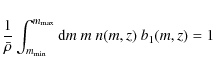
where n(m) is the halo mass function and p(c|m) is the concentration probability distribution for halos given a mass m.

4.2 Ingredients

The halo model approach provides a scale-dependent description of the statistical properties of the large-scale structure. On small scales, the correlation of dark matter is governed by the mass profiles of the halos, whereas on large scales the clustering between different halos determines the nature of the correlation. As there are a multitude of models to describe the behavior on different scales, and an even larger number of parameters one has to set judiciously, there exists no such thing as a unique halo model. In order to have reproducible results, it is therefore necessary to specify ones choice of parameters. For this work, we will adopt the following parameters for the halo model:

1.

The average mass of a halo is defined as the mass within a sphere of virial radius $r_{\rm vir}$ as $m\equiv(4\pi/3)r_{\rm vir}^3 ~ \Delta_{\rm vir} ~ \bar\rho$ , where $\Delta_{\rm vir}$ denotes the overdensity of the virialized halo with respect to the average comoving mass density $\bar\rho$ in the Universe. Typically, values for $\Delta_{\rm vir}$ are derived in the framework of the non-linear spherical collapse model (e.g. Gunn & Gott 1972). Expressions valid for different cosmologies are summarized in Nakamura & Suto (1997). In our implementation, we use the results which are valid for a flat ${\Lambda }$ CDM-Universe, i.e.,

$\begin{displaymath}% \Delta_{\rm vir}(z) = 18\pi^2(1+0.4093 x^{2.71572}), \end{displaymath}$

(22)

where $x \equiv (\Omega_{\rm m}^{-1}-1)^{1/3}/(1+z)$ . We find for our fiducial WMAP5-like cosmology $\Delta_{\rm {vir}}(z=0)=349$ .

2.

N-body simulations suggest that the density profile of a halo follows a universal function. We choose to use the NFW profile (Navarro et al. 1997), which is in good agreement with numerical results and has an analytical Fourier transform. It is given by

$\begin{displaymath}% \rho(r,m) = \frac{\rho_{\rm s}}{(r/r_{\rm s})(1+r/r_{\rm s})^2}, \end{displaymath}$

(23)

where $\rho_{\rm s}$ is the amplitude of the density profile and $r_{\rm s}$ characterizes the scale at which the slope of the density profile changes. For small scales ( $r \la r_{\rm s}$ ) the profile scales with $\rho \propto r^{-1}$ , whereas for large scales it behaves as $\rho \propto r^{-3}$ . The Fourier transform of the NFW profile is

$\displaystyle % \tilde{u}(k;m,c)$	=	$\displaystyle \int {\rm d}^3 x ~ \rho({\vec x}; m,c) ~ {\rm e}^{\rm i {\vec k} \cdot {\vec x}} \Bigg/ \int {\rm d}^3 x ~ \rho({\vec x}; m,c)$
	=	$\displaystyle \int_0^{r_{\rm vir}} {\rm d}r ~ 4\pi r^2 \frac{\sin(kr)}{kr} \frac{\rho(r;m,c)}{m}$
	=	$\displaystyle \left[\ln(1\!+\!c) \!-\! \frac{c}{1\!+\!c} \right]^{-1} \Big\{ \sin\eta \left[ {\rm Si}([1\!+\!c] \eta) \!-\! {\rm Si}(\eta) \right]$
		$\displaystyle + ~ \cos\eta \left[ {\rm Ci}([1+c] \eta)\! -\! {\rm Ci}(\eta) \right] - \frac{\sin(c\eta)}{(1+c) \eta} \Big\},$	(24)

where $\eta \equiv k r_{\rm vir}/c$ , we truncated the integration at $r_{\rm vir}$ in the second step, and introduced the concentration parameter $c\equiv r_{\rm vir}/r_{\rm s}$ in the third step. Additionally, we use for the sine- and cosine integrals the definitions

$\begin{displaymath}% {\rm Ci}(x) = - \int_x^\infty \frac{\cos t}{t} ~ {\rm d}t,\qquad {\rm Si}(x) = \int_0^x \frac{\sin t}{t} ~ {\rm d}t. \end{displaymath}$

(25)

3.

The abundance of halos of mass m at a redshift z is given by

$\begin{displaymath}% n(m,z)=\frac{\bar{\rho}}{m^{2}}~ \frac{{\rm d}\ln\nu}{{\rm d}\ln m} ~\nu f(\nu), \end{displaymath}$

(26)

where we introduced the dimensionless variable $\nu=\nu(m,z)$ ,

$\begin{displaymath}% \nu(m,z) \equiv \frac{\delta_{\rm {sc}}(z)}{D(z)\sigma(m)}, \end{displaymath}$

(27)

where D(z) denotes the redshift-dependent growth factor, $\sigma^2(m)$ is the smoothed variance of the density contrast, and $\delta_{\rm sc}(z)$ denotes the value of a spherical overdensity that collapses at a redshift z as calculated from linear perturbation theory. In our work, we use the expression from Nakamura & Suto (1997), which is valid for a ${\Lambda }$ CDM Universe,

$\begin{displaymath}% \delta_{\rm sc}(z) = \frac{3(12\pi)^{2/3}}{20} \left[1-0.0123 \ln(1+x^3)\right], \end{displaymath}$

(28)

where $x \equiv (\Omega_{\rm m}^{-1}-1)^{1/3}/(1+z)$ . The quantity has only a weak dependence on redshift and we find $\delta_{{\rm sc}}(z=0)=1.675$ for our fiducial model.

The advantage of introducing $\nu$ is that part of the mass function can be expressed by the multiplicity function $\nu f(\nu)$ , which has a universal shape, i.e., is independent of cosmological parameters and redshift. In this work, we employ the Sheth and Tormen mass function (Sheth & Tormen 1999)

$\begin{displaymath}% \nu f(\nu) = A(p) \left[1+(q\nu^2)^{-p} \right] \sqrt{\frac{2q}{\pi}} ~ \nu \exp{(-q\nu^2/2)}, \end{displaymath}$

(29)

which is an improvement over the original Press-Schechter formulation (Press & Schechter 1974). We use the parameter values p=0.3, q=0.707, and amplitude A(0.3)=0.322, which follows from mass conservation.

4.

The concentration parameter $c\equiv r_{\rm vir}/r_{\rm s}$ characterizes the form of the halo profile. From N-body simulations one finds that the average, $\bar{c}$ , depends on the halo mass (Bullock et al. 2001) like

$\begin{displaymath}% \bar{c}(m,z) = \frac{c_*}{1+z} \left(\frac{m}{m_*}\right)^{-\alpha}, \end{displaymath}$

(30)

where m_*=m_*(z=0) is the characteristic mass defined within the Press-Schechter formalism as $\delta_{\rm sc}(z=0)= \sigma(m_*)$ . In the following, we will use the values c_*=10 and $\alpha=0.2$ as proposed by Takada & Jain (2003). This implies that more massive halos are less centrally concentrated than less massive ones. However, results from numerical N-body simulations (Bullock et al. 2001; Jing 2000) indicate that there is a significant scatter in the concentration parameter for halos of the same mass. Furthermore, Jing (2000) proposes that such a concentration distribution can be described by a log-normal distribution

$\begin{displaymath}% p(c\vert m) {\rm d}c = \frac{1}{\sqrt{2\pi\sigma^2_{\ln c}}... ...ln c - \ln \bar c)^2}{2\sigma^2_{\ln c}}\right] {\rm d}\ln c. \end{displaymath}$

(31)

Typical values for the concentration dispersion range from $\sigma_{\ln c}=0.18$ to $\sigma_{\ln c}=0.32$ (Wechsler et al. 2002; Jing 2000). Note that the width of the distribution $\sigma_{\ln c}$ is independent of the halo mass. The variation of the halo concentration can be attributed to the different merger histories of the halos (Wechsler et al. 2002). We will analyze the impact of this effect on different spectra in Sect. 4.7. When we use only the mean concentration parameter, we have to replace the probability distribution of the concentration, needed for example in Eq. (21), by a Dirac delta distribution

$\begin{displaymath}% p(c\vert m) {\rm d}c = \delta_{\rm {D}}(c-\bar{c}) ~c ~ {\rm d}\ln c. \end{displaymath}$

(32)

5.

On large scales, the correlation of the dark matter density field is governed by the spatial distribution of halos. Since the clustering behavior of halos and matter density differ, one introduces the bias factors b_i(m,z) such that

$\begin{displaymath}% \delta_{\rm h}(\delta) \equiv \delta_{\rm h}({\vec x};m,z) ... ...ta({\vec x}) + \frac{b_2(m,z)}{2} \delta^2({\vec x}) + \dots \end{displaymath}$

(33)

In this way, the halo density contrast, $\delta_{\rm h}(\delta)$ , is expressed as a Taylor expansion of the matter density contrast, $\delta({\vec x})$ . The bias parameters are in general derived based on the Sheth-Tormen mass function introduced above. For the linear halo bias one obtains then

$\begin{displaymath}% b_1(m,z)= 1 + \frac{q[\nu(m,z)]^{2} -1}{\delta_{\rm sc}(z)} + \frac{2p}{\delta_{\rm sc}(z)[1+(q[\nu(m,z)]^{2})^p]},~~ \end{displaymath}$

(34)

where p and q match the values used in the mass function. Expressions for higher-order bias factors can be found, e.g., in Scoccimarro et al. (2001). Since they only have a small impact on the quantities employed here, we take into account only the first-order bias. In Fourier space we may then write

$\begin{displaymath}% \tilde{\delta}_{\rm h}(\tilde{\delta}) \equiv \tilde{\delta}_{\rm h}(k;m,z) = b_1(m,z) \tilde{\delta}(k). \end{displaymath}$

(35)

6.

To obtain the final correlation function, one has to perform integrations along the halo mass and optionally along the halo concentration, with limits formally extending from 0 to $\infty$ . In practice, we use the mass limits $m_{\rm min}=10^3~h^{-1}~M_\odot$ and $m_{\rm max}=10^{16}~h^{-1}~M_\odot$ . Masses smaller than $m_{\rm min}=10^3~h^{-1}~M_\odot$ give no significant contribution to the considered quantities, while, due to the exponential cut-off in mass, masses larger than $m_{\rm max}=10^{16}~h^{-1}~M_\odot$ are rare. For the concentration, we employ the integration limits $c_{\rm min}=1$ and $c_{\rm max}=10^3$ .

7.

Due to the cut-off in mass, the consistency relation (Scoccimarro et al. 2001)

$\begin{displaymath}% \frac{1}{\bar{\rho}}\int_{m_{\rm min}}^{m_{\rm max}} {\rm d}m ~ m ~ n(m,z) ~ b_{1}(m,z) = 1 \end{displaymath}$

(36)

does not hold. To cure this problem we consider a rescaled linear bias such that $b_{1}(m,z) \rightarrow b_{1}(m,z)/b_{\rm norm}(z)$ , where $b_{\rm norm}(z)$ is the result of the integral in Eq. (36). In this way, one ensures that the halo term with the largest contribution to the correlation equals the perturbation theory expression on large scales (see Fig. 1).

4.3 Building blocks

Using the ingredients described in the previous section, it is possible to define building blocks, which simplify significantly the notation for expressing the polyspectra (Cooray & Hu 2001):

$\displaystyle % M_{ij} (k_1,\ldots,k_j;z)$	$\textstyle \equiv$	$\displaystyle \int_{m_{\rm min}}^{m_{\rm max}} {\rm d}m ~ \int_{c_{\rm min}}^{c_{\rm max}} {\rm d}c ~ n(m,z) ~ p(c\vert m) \left(\frac{m}{\bar\rho}\right)^j$
		$\displaystyle \times ~ b_i(m,z) ~ [\tilde{u}(k_1;m,c) \cdots \tilde{u}(k_j;m,c)].$	(37)

In the case i=0, we additionally define $b_0 \equiv 1$ , for consistency.

$\begin{figure} \par\includegraphics[width=12cm,clip]{12854fg1} \end{figure}$

Figure 1:

Square configuration of the dimensionless convergence trispectrum ${\cal T}^n_\kappa (\ell )$ against wave-number $\ell$ for the range $10 \leq \ell \leq 10^4$ for $n \in \{\mbox{1h, 2h, 3h, 4h, tot, pt}\}$ . The upper panel displays the four individual halo terms, the sum of all four trispectrum halo terms ${\cal T}^{\rm tot}_\kappa$ (solid line) and the tree-level perturbation theory trispectrum ${\cal T}^{\rm pt}_\kappa$ , as indicated in the key. The lower panel shows the ratio between the indicated contributions and the complete trispectrum. The double dashed line illustrates the corresponding ratio of the approximation ${\cal T}^{\rm tot}_\kappa \approx {\cal T}^{\rm pt}_\kappa + {\cal T}^{\rm 1h}_\kappa$ . Note that we consider the 4-halo term only in the upper panel since it resembles the term ${\cal T}^{\rm pt}_\kappa$ on large scales.

Open with DEXTER

4.4 Power spectrum

We can now compute the power spectrum from Eq. (20). The result consists of two terms, the 1-halo and the 2-halo terms, $P_\delta(k)=P_{\rm 1h}(k)+P_{\rm 2h}(k)$ (Seljak 2000). They are given by

$\displaystyle P_{\rm 1h}(k)$	=	$\displaystyle \frac{1}{\bar\rho^2} \! \int_{m_{\rm min}}^{m_{\rm max}} {\rm d}m... ... min}}^{c_{\rm max}} {\rm d}c ~ p(c\vert m) ~ ~ \vert\tilde{u}(k;m,c)\vert^2,~~$	(38)
$\displaystyle P_{\rm 2h}(k)$	=	$\displaystyle \left[ \frac{1}{\bar\rho}\! \int_{m_{\rm min}}^{m_{\rm max}} {\rm... ..._{\rm min}}^{c_{\rm max}} {\rm d}c ~ ~ p(c\vert m) ~ \tilde{u}(k;m,c) \right]^2$
		$\displaystyle \times ~ P_{\rm lin}(k),$	(39)

where $P_{\rm lin}(k)$ denotes the linear perturbation theory power spectrum, defined in Eq. (4), and we use the ingredients summarized earlier-on. Note that, for convenience, we omit the redshift-dependence in the notation. Using the building blocks from Eq. (37), these terms can be written in the following compact form:

$\displaystyle % P_{\rm 1h}(k) = M_{02}(k,k), \qquad P_{\rm 2h}(k) = [M_{11}(k)]^2 P_{\rm lin}(k).$

(40)

The 1-halo term, $P_{\rm 1h}$ , denotes correlations in space between two points in the same halo, whereas the 2-halo term, $P_{\rm 2h}$ , takes into account correlations between two different halos. Hence, the 1-halo term is dominant on small scales and the 2-halo term is dominant on large scales. Note that the 2-halo term converges to the linear power spectrum on large scales because of the consistency relation of the first-order halo bias factor (see Eq. (36)) and of the limit $\tilde{u}(k;m,c) \rightarrow 1$ for $k \rightarrow 0$ .

4.5 Trispectrum

We compute now the dark matter trispectrum in the halo model approach. As discussed in Sect. 3, only parallelogram configurations of the trispectrum wave-vectors contribute to the covariance of the convergence power spectrum. Restricting our calculations to these configurations, we obtain four different halo term contributions,

$\begin{displaymath}% T_{\delta}(k_1,k_2,\cos \varphi) = T_{\rm 1h}+T_{\rm 2h}+T_{\rm 3h}+T_{\rm 4h}, \end{displaymath}$

(41)

which are simpler than in the general case. In addition, we neglect terms involving higher-order halo bias factors since, on most scales, they provide only a small correction (Takada & Jain 2003; Ma & Fry 2000). We further note that the perturbative expansion of halo centers, used in the calculations, was shown to become inaccurate on non-linear scales (Smith et al. 2007). The contributions to the trispectrum take the following forms, using the compact notation of the building blocks (see Cooray & Sheth 2002, for the expression of the halo model trispectrum including higher-order bias factors): The 1-halo term, dominant on the smallest scales, is

$\begin{displaymath}% T_{\rm 1h} = M_{04}(k_1,-k_1,k_2,-k_2). \end{displaymath}$

(42)

The 2-halo term has two contributions, $T_{\rm 2h} = T_{\rm 2h}^{31} + T_{\rm 2h}^{22}$ , consisting of a term $T_{\rm 2h}^{31}$ , which corresponds to correlations of three points within one halo and a fourth point in a second halo, and a term $T_{\rm 2h}^{22}$ , which describes correlations involving two points in a first halo and the other two points in the second halo. They read,

$\displaystyle % T_{\rm 2h}^{31}$	=	$\displaystyle 2 M_{13}(k_1,k_2,k_2) M_{11}(k_1) P_{\rm lin}(k_1)$
		$\displaystyle + ~ 2 M_{13}(k_1,k_1,k_2) M_{11}(k_2) P_{\rm lin}(k_2),$	(43)
$\displaystyle T_{\rm 2h}^{22}$	=	$\displaystyle M_{12}^2(k_1,k_2) [P_{\rm lin}(\vert{\vec k}_1+ {\vec k}_2\vert) + P_{\rm lin}(\vert{\vec k}_1 - {\vec k}_2\vert)].$	(44)

The 3-halo term is given by

$\displaystyle % T_{\rm 3h}$	=	2 M₁₂(k₁,k₂) M₁₁(k₁) M₁₁(k₂)
		$\displaystyle \times ~ \left[B_{\rm pt}({\vec k}_1,{\vec k}_2,- {\vec k}_1 - {\vec k}_2) + B_{\rm pt}({\vec k}_1,-{\vec k}_2,- {\vec k}_1 + {\vec k}_2) \right].$	(45)

Finally, the 4-halo term, dominant on large scales, is

$\begin{displaymath}% T_{\rm 4h} = M^2_{11}(k_1) M^2_{11}(k_2) T_{\rm pt}({\vec k}_1,- {\vec k}_1,{\vec k}_2, -{\vec k}_2), \end{displaymath}$

(46)

and describes correlations of points distributed in four different halos. Note that, like for the power spectrum, the 2-halo term is computed from the linear power spectrum. On the other hand, the 3- and 4-halo terms depend on $B_{\rm pt}$ and $T_{\rm pt}$ , respectively, which are the lowest-order, non-vanishing, perturbation theory contributions to the bispectrum and trispectrum. Both spectra are derived in Appendix A.2.

4.6 Convergence spectra

The convergence power spectrum and trispectrum, needed to evaluate the covariance in Eq. (14), are computed by projecting $P_\delta$ and $T_\delta$ , according to Eqs. (10) and (11). Figure 1 shows the dimensionless convergence trispectrum, defined as ${\cal T}_\kappa^n(\ell)= \ell^2/2\pi ~ \sqrt[3]{T_\kappa^n({\vec \ell}, -{\vec \ell}, {\vec \ell}, -{\vec \ell})}$ for a square configuration where all wave-numbers have a length $\ell$ , where $n \in \{ \rm 1h,2h,3h,4h\}$ denotes the contribution from the corresponding halo term. The plot shows the individual contributions to the dimensionless ${\cal T}_\kappa^n$ (the projections of Eqs. (42)-(46)), illustrating on which scales the individual terms are important, as well as the total contribution of all halo terms ${\cal T}^{\rm tot}_\kappa$ . We show, in addition, the dimensionless projected ${\cal T}^{\rm pt}_\kappa$ , which closely follows the 4-halo term. We see that the commonly used approximation ${\cal T}^{\rm tot}_\kappa \approx {\cal T}^{\rm pt}_\kappa + {\cal T}^{\rm 1h}_\kappa$ is accurate for large wave-numbers ( $\ell \ga 10^3$ ) but has a deviation of about $20\%$ from the complete trispectrum ${\cal T}^{\rm tot}_\kappa$ for small wave-numbers ( $\ell \la 10^2$ ).

4.7 Stochastic halo concentration

The previous results were computed using the deterministic concentration-mass relation of Eq. (30). We now analyze the impact of scatter in the halo concentration parameter c on the covariance of the convergence power spectrum, using the stochastic concentration relation given by the the log-normal concentration distribution of Eq. (31).

Cooray & Hu (2001), analyzed the effect of a stochastic concentration on the three-dimensional power spectrum and trispectrum and found that the behavior of the corresponding 1-halo terms were increasingly sensitive to the width of the concentration distribution for smaller wave-numbers k. Furthermore, the effect of a stochastic concentration relation was more pronounced for the trispectrum than for the power spectrum, since the tail of the concentration distribution is weighted more strongly in higher-order statistics.

Performing the same analysis for the projected power spectrum and trispectrum, we find a similar trend as in the three-dimensional case, but with a smaller sensitivity to the concentration width of the distribution on small scales. For $\sigma_{\ln c}=0.3$ , we find, in the case of the 1-halo term of the power spectrum, a deviation from a deterministic concentration relation of about $1{-}2\%$ for wave-numbers larger than $\ell \sim 10^3$ , whereas, for the 1-halo term of the trispectrum, the deviation is of the order of $10{-}15\%$ in the same $\ell$ -range. Thus, when considering the covariance of the convergence power spectrum, one should take into account the concentration dispersion in the 1-halo term of the trispectrum but can safely neglect it for the power spectrum. Additionally, we find that a stochastic concentration has only a small impact on the 2-halo terms of the power spectrum and trispectrum (Pielorz 2008).

From this analysis, we expect the effect of a concentration distribution to be the strongest on the non-Gaussian part of the covariance, which depends on the trispectrum. To directly infer the impact of a concentration distribution on the covariance, we calculate the 1-halo contribution to the non-Gaussian covariance, i.e., we perform the bin averaging of Eq. (15),

$\begin{displaymath}% \mathcal{C}_{1 \rm h}^{\rm {NG}}(\ell_i,\ell_j) \simeq \in... ..._j)} ~ \ell_2^3 ~ {T}_{\kappa}^{1 \rm h}(\ell_{1},\ell_{2}), \end{displaymath}$

(47)

for two different concentration dispersions $\sigma_{\ln c}$ , using our halo model implementation. Figure 2 shows the ratio

$\begin{displaymath}% R(\ell_i,\ell_j) \equiv \frac{\mathcal{C}_{1 \rm h}^{\rm {... ...thcal{C}_{1 \rm h}^{\rm {NG}}(\ell_i,\ell_j;\sigma_{\ln c})}, \end{displaymath}$

(48)

where $\sigma_{\ln c}=0$ denotes the deterministic concentration relation, for two values $\sigma_{\ln c}=\{0.15,0.3\}$ in two contour plots. In agreement with the previous results, the largest impact of the concentration dispersion occurs for wave-numbers larger than $\ell_i \simeq \ell_j \simeq 4000$ . For $\sigma_{\ln c}=0.15$ , the deviation of the covariance $\mathcal{C}_{1 \rm h}^{\rm {NG}}$ from the original deterministic concentration relation is small, of about $3{-}6\%$ . The effect becomes non-negligible for $\sigma_{\ln c}=0.3$ , where we find a deviation of $12\%$ (for $\ell_i \simeq \ell_j \ga 4000$ ) to $25\%$ (for $\ell_i \simeq \ell_j \ga 8000$ ).

$\begin{figure} \par\includegraphics[width=12cm,clip]{12854fg2} \end{figure}$

Figure 2:

Contour plots of the ratio $R(\ell _i,\ell _j)$ between the non-Gaussian covariance 1-halo term contribution (see Eq. (48)) computed with a concentration dispersion $\sigma_{\ln c}$ and with a deterministic concentration, against wave-numbers $(\ell _i,\ell _j)$ ranging from $\ell _i=\ell _j=500$ to $\ell _i=\ell _j=8500$ . The left panel is for concentration dispersion $\sigma_{\ln c}=0.15$ , whereas in the right panel $\sigma_{\ln c}=0.3$ .

Open with DEXTER

5 Comparison with N-body simulations

In Sect. 4, we computed the power spectrum and trispectrum of the dark matter fluctuations. Projecting them according to Eqs. (10) and (11), and inserting the result in Eqs. (12), (14), and (15), we obtained the covariance of the convergence power spectrum estimator.

To test the accuracy of the halo model predictions for the statistics of the dark matter density field, we compare the dimensionless convergence power spectrum and the corresponding covariance, calculated in the halo model approach, with results from two different ray-tracing simulations.

Table 1: Cosmological parameters used to set up the initial power spectrum.

Table 2: Parameters used for generating the two N-body simulations.

5.1 Virgo and Gems simulation

For our comparison, we chose one simulation from Jenkins et al. (1998) and ten simulations from Hartlap et al. (2009), which we denote in the following as Virgo and Gems simulation, respectively. The Virgo simulation was carried out in 1997 by the Virgo-Consortium for a ${\Lambda }$ CDM cosmology (see Table 1) with $N_{\rm par}=256^3$ particles in a periodic box of comoving side length $L_{\rm box}=141.3~h^{-1}~{\rm Mpc}$ (see Table 2). It uses the PP-/PM-code HYDRA, which places subgrids of higher resolution in strongly clustered regions. Structures on scales larger than $2 l_{\rm soft} \approx 40~h^{-1}~{\rm kpc}$ can be considered as well resolved. The Gems simulations were set up in cubic volumes of comoving side length $L_{\rm box}=150~h^{-1}~{\rm Mpc}$ with 256³ particles (see Table 2). Note that the simulations employ either the BBKS (Bardeen et al. 1986) or the EH (Eisenstein & Hu 1998) transfer function. The cosmology chosen reflects the WMAP5 results (Komatsu et al. 2009) and thus has a lower value for $\sigma_8$ than the Virgo simulation (see Table 1). It uses the GADGET-2 code to simulate the evolution of dark matter particles (Springel 2005) and has a softening length of $2l_{\rm soft} \approx 30~h^{-1}~{\rm kpc}$ .

5.2 Ray-tracing

The output of numerical simulations are three-dimensional distributions of $N_{\rm par}$ particles in cubic boxes over a range of redshift values. In order to compare the results with the predicted convergence power spectrum from the halo model, we make use of the multiple-lens-plane ray-tracing algorithm (see e.g., Jain et al. 2000; Hilbert et al. 2009) to construct effective convergence maps. The basic idea is to introduce a series of lens planes perpendicular to the central line-of-sight of the observer's backward light cone. In this way, the matter distribution within the light cone is sliced and can be projected onto the corresponding lens plane. By computing the deflection of light rays and its derivatives at each lens plane, one simulates the photon trajectory from the observer to the source by keeping track of the distortions of ray bundles. In this way, the continuous deflection of light rays is approximated by a finite number of deflections at the lens planes. As a result, one obtains the Jacobian matrix for the lens mapping from source to observer and can construct convergence maps.

For both simulations, a similar number of around 200 effective convergence maps were produced, with source galaxies situated at a single redshift of either $z_{\rm s}=1$ or $z_{\rm s}=2$ . Table 2 summarizes the parameters used for producing the resulting convergence maps with the multiple-lens-plane-ray-tracing-algorithm. These are: the side length, $L_{\mbox{\scriptsize box}}$ , of the cubic simulation box, the number of particles, $N_{\mbox{\scriptsize par}}$ , used for the simulation, their mass, $m_{\mbox{\scriptsize par}}$ , and the number of available convergence maps, $N_{\mbox{\scriptsize map}}$ , with area $A_{\mbox{\scriptsize map}}$ .

The maps produced with the Gems simulation have an area of 16 $\deg^2$ , while the ones from Virgo are much smaller, with 0.25 $\deg^2$ .

$\begin{figure} \par\hspace*{0.25mm}\includegraphics[width=11.9cm,clip]{12854fg3}... ...e*{0.25mm}\vspace*{3mm} \includegraphics[width=12cm,clip]{12854fg4} \end{figure}$

Figure 3:

Dimensionless convergence power spectrum ${\cal P}_\kappa (\ell )$ against wave-number $\ell$ for galaxy sources at redshift $z_{\rm s}=1$ ( upper panels) and $z_{\rm s}=2$ ( lower panels). Points with error bars show measurements from the two sets of numerical simulations: Gems (left plots) and Virgo (right plots). Both simulations use a similar particle setup but differ in the area of the $\kappa$ -maps (see Tables 1 and 2). They are compared with the corresponding results obtained with fitting formulae from Smith et al. (long-dashed line), Peacock-Dodds (short-dashed line), and the halo model predictions for a deterministic halo concentration (solid line). See text for a discussion.

Open with DEXTER

5.3 Convergence power spectrum

To test the accuracy of the halo model approach in describing the non-linear evolution of dark matter, we compare the dimensionless projected power spectrum, computed in the halo model approach, to the ones estimated from the numerical N-body simulations.

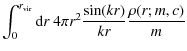
The dimensionless convergence power spectra of the simulations are measured from the real-space two-dimensional convergence maps of length $L_{\rm map}$ and grid-size $N_{\rm bin}$ . For this, we first apply a Fast Fourier Transform to obtain $\tilde{\kappa}(\ell)$ on each grid-point. Then, we estimate the power spectrum at a wave-number $\ell$ for the kth convergence map by averaging over all Fourier modes in the band ${{\vec \ell}}_{\rm b}=\{{\vec \ell} ~ \vert ~ \ell-\Delta \ell/2 \leq \vert{\vec \ell}\vert \leq \ell+\Delta \ell/2$ }, i.e.,

$\begin{displaymath}% \hat{\cal P}^{(k)} (\ell)= \frac{1}{N_{\rm p}(\ell)} \sum_{... ... b}} \frac{\ell^2}{2\pi} ~ \vert\tilde{\kappa}(\ell)\vert^2, \end{displaymath}$

(49)

where $N_{\rm p}(\ell)$ denotes the number of modes in each band $\ell_{\rm b}$ of width $\Delta \ell$ . Finally, the ensemble average of the dimensionless power spectrum is obtained by averaging over the results of the various convergence maps, i.e., $\mathcal{P}(\ell) = \frac{1}{N_{\rm map}} \sum_{k=1}^{N_{\rm map}} \hat{\cal P}^{(k)}(\ell_i)$ . The error bars for the power spectrum estimate are computed from the dispersion over the $N_{\rm map}$ convergence maps used, and are due to sample variance. Since modes with a length similar to the side length of the convergence map are only poorly represented, the sampling variance is largest for small $\ell$ . The effect is stronger for the Virgo simulation than for the Gems simulation, since the Gems convergence maps have a much larger area $A_{\rm map}$ .

Figure 3 shows a good agreement between the halo model and the N-body simulation convergence power spectra. We also include, in Fig. 3, the convergence power spectra computed using the fitting formulae of Peacock & Dodds (1996) and Smith et al. (2003). Both, the halo model and the fitting formulae, show a better agreement with simulations for the lower source redshift case. On small scales, the halo model and the Smith et al. fitting formula agree well with the simulations, whereas the Peacock-Dodds fitting formula has too little power, in particular in the case of the Gems simulation. On intermediate scales ( $\ell \simeq 10^3$ ), the halo model is less accurate than the Smith et al. fitting formula, suggesting that the halo model suffers from the halo exclusion problem on these scales, as described, e.g., in Tinker et al. (2005). This means that, while in simulations halos are never separated by distances smaller than the sum of their virial radii, this is not accounted for in the framework of our halo model and is probably the cause for the deviation. The good agreement of the Smith et al. formula is not surprising, since it is based on simulations of similar resolution than the ones we consider here. In contrast, a similar comparison using the convergence power spectrum estimated with the Millennium Run (Hilbert et al. 2009) clearly favors the halo model prediction over of the two fitting formulae, with both fitting formulae strongly underestimating the power on intermediate and small scales.

The good overall accuracy of the halo model results was expected since its ingredients, such as the mass function and the halo profile, were obtained from N-body simulations. We note that, in this analysis, we used a deterministic concentration parameter, since the use of a stochastic one has only a small effect on the small scales of the convergence power spectrum.

5.4 Covariance of the convergence power spectrum

The similarity between simulation and halo model power spectra was to some extent expected. The ability to make an accurate description of higher-order correlations provides a stronger test of the halo model. Due to its important role in calculating the error of the power spectrum and for parameter estimates, we focus in this section on the accuracy of the covariance of the dimensionless convergence power spectrum.

We need an appropriate estimator for the power spectrum covariance of the simulations. As each simulation provides $N_{\rm map}$ different $\kappa$ -maps, we have $N_{\rm map}$ realizations of the power spectrum. From these we estimate the covariance by applying the unbiased sample covariance estimator which has for our purpose the form:

$\displaystyle % C_{\rm sim}(\ell_i,\ell_j)$	=	$\displaystyle \frac{1}{N_{\rm map}-1} \times \Bigg[ ~ \sum_{k=1}^{N_{\rm map}} \hat{\cal P}_\kappa^{(k)}(\ell_i) \hat{\cal P}_\kappa^{(k)}(\ell_j)$
		$\displaystyle - ~ \frac{1}{N_{\rm map}} \Bigg(\sum_{k=1}^{N_{\rm map}} \hat{\ca... ...gg( \sum_{k=1}^{N_{\rm map}} \hat{\cal P}_\kappa^{(k)}(\ell_j) \Bigg) ~ \Bigg],$	(50)

where $\hat{\cal P}_\kappa^{(k)}(\ell_i)$ is the projected power spectrum estimate of the kth effective convergence map at a wave-number $\ell_i$ (see Eq. (49)). We evaluate $C_{\rm sim}$ for both, Virgo and Gems simulations, for the case $z_{\rm s}=1$ .

The halo model results, $\mathcal{C}_{\rm halo}$ , are calculated as described in Sect. 4 and include all terms of the non-Gaussian covariance. In their computation, we use our fiducial halo model with the ingredients summarized in Sect. 4.2, and use the cosmological parameters values corresponding to each simulation, given in Table 1, for the case $z_{\rm s}=1$ . We consider both, a deterministic concentration-mass relation and a stochastic one, with dispersion $\sigma_{\ln c}=0.3$ for the 1-halo term of the trispectrum.

$\begin{figure} \par\includegraphics[width=15cm,clip]{12854fg5} \end{figure}$

Figure 4:

Relative difference $\Delta \mathcal{C}_{ij}/\mathcal{C}_{ij}$ (see Eq. (51)) between the halo model prediction for the covariance of the convergence power spectrum and the results from the Virgo simulation ( $z_{\rm s}=1$ ) against wave-numbers $(\ell _i,\ell _j)$ . The binning scheme is linear with a constant bin width of $\Delta l=720$ ranging from $\ell _0=720$ to $\ell _{20}=15120$ . The left panel displays the full covariance, including all four halo terms for the trispectrum, and uses a deterministic concentration-mass relation denoted by $\sigma_{\ln c}=0$ . The right panel illustrates the same covariance but with a stochastic concentration distribution of width $\sigma_{\ln c}=0.3$ for the 1-halo term of the trispectrum.

Open with DEXTER

$\begin{figure} \par\includegraphics[width=15cm,clip]{12854fg6} \end{figure}$

Figure 5:

Relative difference $\Delta \mathcal{C}_{ij}/\mathcal{C}_{ij}$ (see Eq. (51)) between the halo model prediction for the covariance of the convergence power spectrum and the results from the Gems simulation ( $z_{\rm s}=1$ ) against wave-numbers $(\ell _i,\ell _j)$ . The binning scheme is linear with a constant bin width of $\Delta l=90$ ranging from $\ell _0=90$ to $\ell _{20}=7020$ . The left panel displays the full covariance, including all four halo terms for the trispectrum, and uses a deterministic concentration-mass relation denoted by $\sigma_{\ln c}=0$ . The right panel illustrates the same covariance but with a stochastic concentration distribution of width $\sigma_{\ln c}=0.3$ for the 1-halo term of the trispectrum.

Open with DEXTER

We compare the halo model with the simulations covariance matrices considering their relative deviation

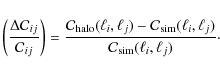
$\begin{displaymath}% \left(\frac{\Delta \mathcal{C}_{ij}}{\mathcal{C}_{ij}}\righ... ...im}(\ell_i,\ell_j)}{\mathcal{C}_{\rm sim}(\ell_i,\ell_j)}\cdot \end{displaymath}$

(51)

We note that although the number of available convergence maps for our simulations ( ${\sim}200$ ) is too small to obtain a percentage level accuracy for the covariance estimate (Takahashi et al. 2009), we assume that the covariance from the simulations is the reference one, and put it in the denominator of Eq. (51). The comparisons are displayed in Figs. 4 and 5 for the Virgo and Gems simulation, respectively. In the case of the Virgo simulation with $\sigma_{\ln c}=0$ , the best agreement is a relative deviation of $20{-}40\%$ found on intermediate scales between $\ell \simeq 1500$ and $\ell \simeq 5000$ . For small scales $(\ell \ga 6000)$ the halo model underestimates the simulation by $60\%$ or more. On large scales, i.e., for wave-numbers $\ell \la 1500$ , the halo model overestimates the simulation by around $60\%$ . However, since the simulation covariances suffer from a large sampling variance due to the small size of the convergence maps, the comparison is not meaningful on these scales. The agreement improves for $\sigma_{\ln c}=0.3$ , in this case there is a larger range of scales where the deviation is small. For the Gems simulation the agreement is much better. There is now an interval of scales ( $\ell \la 1500$ ) where the deviation is in the range $0{-}40\%$ . Throughout all the scales probed, the deviation on the diagonal of the covariances is around $20{-}40\%$ . However, for off-diagonal components, at small scales, the agreement is still poor. Finally, the improvement of considering $\sigma_{\ln c}=0.3$ is less significant than in the Virgo case.

Although the halo model predictions strongly deviate from the simulation estimates of the covariance on small scales, this analysis does not necessarily imply a poor accuracy of those predictions. Indeed, the simulation covariances estimated in this analysis have a strong scatter. In particular, in the case of the Gems simulation, we found from bootstrap subsamples of 50 convergence maps that the resulting covariances can deviate up to $20\%$ from the average covariance of the complete sample (Pielorz 2008). This is in agreement with the results by Takahashi et al. (2009) who need to use 5000 simulations to obtain an estimate of the matter power spectrum covariance at a sub-percent level accuracy.

There are however very recent indications that Eq. (14) indeed underestimates the covariance of the convergence power spectrum on small scales (Sato et al. 2009). In particular, sample variance in the number of halos in a finite field is not accounted for by Eq. (14). Indeed, the mass function yields a mean number density, but there are fluctuations on the number of halos due to the large-scale mass fluctuations. Sample variance in the number of clusters in a volume-limited survey (Hu & Kravtsov 2003) has been considered in cluster abundance studies (e.g., Vikhlinin et al. 2009). In the halo model framework, the sample variance in the number of halos was derived in Takada & Bridle (2007) and its contribution to the covariance of the convergence power spectrum was found, in Sato et al. (2009), to boost the non-Gaussian errors of a 25 $\deg^2$ survey by one order of magnitude on scales $\ell \approx 10^4$ . The increase is reduced for larger survey areas.

6 Fitting formula for the covariance of the convergence power spectrum

Future weak lensing surveys will provide much more precise measurements of the convergence power spectrum. In order to obtain robust constraints on cosmological parameters, accurate estimates of both the power spectrum and its covariance are needed.

6.1 Methodology

The number of measured power spectra is, in general, insufficient to infer the complete covariance directly from observations. One has thus to derive it either from ray-tracing maps of numerical N-body simulations or with an analytic approach. A drawback of the first method is that it requires a large number of realizations and, in addition, is very time-consuming if an exploration of the covariance in the parameter space is needed.

In the previous sections, we derived the covariance, and in particular its non-Gaussian part, with an analytic approach. This computation is, however, time-consuming and it might be useful to obtain an accurate covariance in a faster way. A first approach would be to rely on stronger approximations. For example, a commonly used approximation consists on evaluating the non-Gaussian covariance from $T_\kappa \approx T_{\rm pt} + T_{\rm 1h}$ , instead of using the full trispectrum. We saw in Sect. 4 that this approximation recovers the full trispectrum for scales $\ell \ga 10^3$ but deviates by ${\sim}40\%$ on scales $\ell \la 10^2$ for square configurations (compare also with Fig. 6).

An alternative approach that we consider in the following, is to find a fitting formula for the halo model covariance that can be subsequently used without the need for implementing the halo model. We will provide a fit only for the non-Gaussian part of the halo model covariance, since the Gaussian part only depends on the non-linear convergence power spectrum and can thus be accurately computed without relying on the halo model. The inclusion of non-Gaussian errors increases the total covariance and one might think of fitting the ratio between the non-Gaussian and Gaussian terms. However, this is not a good quantity to fit, since the Gaussian contribution is diagonal and binning-dependent. In contrast, a similar ratio was fitted in the real space, where the Gaussian term is non-diagonal and binning-independent, using a non-Gaussian contribution measured from N-body simulations (Semboloni et al. 2007). In Fourier space, there is some relevant analogous information contained in the tree-level perturbation theory trispectrum. Indeed, pursuing the analogy with the real-space fit, $T_{\rm pt}$ is a non-diagonal and binning-independent quantity, with a lower amplitude than the full trispectrum, approaching it at large scales. We thus compute ${\cal C}_{\rm pt}$ , the covariance predicted in tree-level perturbation theory on large scales (see Eq. (A.27) and Appendix A for a detailed derivation) and compare it with our covariance computed with the full halo model trispectrum, ${\cal C}^{\rm NG}$ , defined in Eq. (14). The ratio between the two covariances is shown in Fig. 6. In agreement with Fig. 1, the covariance predicted by tree-level perturbation theory contributes only ${\sim}50\%$ to the complete non-Gaussian covariance along the diagonal. On very large scales $(\ell<100)$ , the ratio ${\cal C}^{\rm NG}/{\cal C}_{\rm pt}$ lies between 1.1 and 2. On smaller scales, ${\cal C}_{\rm pt}$ decreases fast and is no longer useful for fitting purposes.

$\begin{figure} \par\includegraphics[width=9cm,clip]{12854fg7} \end{figure}$

Figure 6:

Ratio ${\cal C}_{\rm pt}/{\cal C}^{\rm NG}$ against wave-numbers $(\ell _i,\ell _j)$ . The covariance in tree-level perturbation theory resembles the non-Gaussian covariance on very large scales (i.e., $\ell _i=\ell _j\leq 20$ ) to approximately $80{-}90\%$ except along the diagonal and the closest off-diagonals. Here a good approximation of the non-Gaussian covariance requires at least one additional halo term. For wave-numbers $\ell _i=\ell _j\geq 100$ , an accurate description of the non-Gaussian covariance requires at least the 1-halo term.

Open with DEXTER

This discussion motivates us to use two different fitting formulae to model the non-Gaussian covariance over the whole range of scales. On large scales ( $1<\ell<200$ ), we model the ratio ${\cal C}^{\rm NG}/{\cal C}_{\rm pt}$ as a polynomial in the wave-numbers, $\ell_i~,\ell_j$ , and the dimensionless non-linear convergence power spectrum $\mathcal{P}_\kappa(\ell)$ . More precisely, we assume

$\displaystyle % \mathcal{C}_< (\ell_i,\ell_j)$	=	$\displaystyle \mathcal{C}_{\rm pt}(\ell_i,\ell_j) ~ \Big[ ~ 1.1 + a_0 \ell_{\rm min} + a_1 \ell_{\rm max} + a_2 {\mathcal{P}_\kappa(\ell_{\rm min})}$
		$\displaystyle + ~ a_3 {\mathcal{P}_\kappa(\ell_{\rm max})} ~ \Big],$	(52)

where $\ell_{\rm min}= \min(\ell_i, \ell_j)$ and $\ell_{\rm max}=\max(\ell_i, \ell_j)$ which ensures the symmetry property $\mathcal{C}_{<}(\ell_i,\ell_j)=\mathcal{C}_{<}(\ell_j,\ell_i)$ . In this way, $\mathcal{C}_{<} \rightarrow 1.1 ~ \mathcal{C}_{\rm pt}$ for large scales as predicted by the halo model (see Fig. 6). On smaller scales, we use the fact that the degree of non-Gaussianity is expected to depend on the amplitude of the dimensionless power spectrum; if the latter is small, only small non-Gaussianities may be expected. In Eq. (52), the non-linear clustering on these scales is thus encoded in the first-order polynomial in wave-numbers and power spectra.

On small scales, i.e. for $200<\ell<8000$ , we model directly the non-Gaussian covariance amplitude using a second-order polynomial in the power spectrum, such that

$\displaystyle % \mathcal{C}_{>}(\ell_i,\ell_j)$	=	$\displaystyle a_4{\mathcal{P}_\kappa(\ell_{\rm min})} + a_5{\mathcal{P}_\kappa(\ell_{\rm max})} + a_6 {\mathcal{P}_\kappa^2(\ell_{\rm min})}$
		$\displaystyle + ~ a_7{\mathcal{P}_\kappa^2(\ell_{\rm max})} + a_8 {\mathcal{P}_\kappa(\ell_{\rm min})}{\mathcal{P}(\ell_{\rm max})}.$	(53)

The scale-dependence of the nonlinear regime of the covariance of the three-dimensional power spectrum is also to some extent captured in powers of the non-linear power spectrum. This assumption is weaker when dealing with projected spectra; due to the redshift projection of the Limber equation, such a relation is not so tight for the corresponding two-dimensional spectra. We verify that nevertheless considering only terms up to second-order in the power spectrum in Eq. (53) already produces an accurate fitting formula in this range of scales, allowing for a better fit with a smaller number of parameters than by using an arbitrary function of wavenumbers.

To ensure a smooth transition from small to large wave-numbers, we consider a linear combination of the two matrices defined in Eqs. (52) and (53) with weightings of third-order in the wave-numbers, such that the full non-Gaussian covariance becomes

$\displaystyle % \mathcal{C}^{\rm NG}_{\rm fit}(\ell_i,\ell_j)$	=	$\displaystyle \frac{\ell_0^3}{\ell_0^3+(\ell_i + \ell_j)^3} ~ \mathcal{C}_{<}(\ell_i,\ell_j)$
		$\displaystyle + ~ \frac{(\ell_i + \ell_j)^3}{\ell_0^3+(\ell_i + \ell_j)^3} ~ \mathcal{C}_{>}(\ell_i,\ell_j),$	(54)

with the transition scale fixed at $\ell_0=600$ . We use thus a model with nine free parameters, which is a compromise between expressive power and simplicity, and perform the fit using the range $1 \leq \ell \leq 8000$ . More precisely, we find the coefficients for the final fit formula by performing two least square fits to Eqs. (52) and (53), respectively. To obtain the coefficients for small (large) scales we computed the corresponding covariance as described above within the halo model approach with 61 bins in the range $10^2 \leq \ell \leq 10^4$ ( $1 \leq \ell \leq 10^3$ ) and employed the condition $\ell_i +\ell_j \geq 200$ ( $\ell_i +\ell_j < 200$ ) for the fit.

The covariances used in the fitting procedure, both tree-level perturbation theory and halo model covariance, depend on perturbation theory polyspectra. These were evaluated from the expressions derived in Appendix A using a linear matter power spectrum computed with the Eisenstein-Hu transfer function (Eisenstein & Hu 1998) and assuming the WMAP5-like fiducial model shown in Table 3. The non-linear convergence power spectrum, used in the polynomial expressions, was evaluated from the same linear power spectrum. In addition, the halo model non-Gaussian covariance was evaluated using the input parameters as described in Sect. 4.2, including a stochastic concentration-mass relation with $\sigma_{\ln c}=0.3$ for the 1-halo term of the trispectrum.

Table 3: Fiducial model used for the fitting procedure.

Table 4: Best-fit values for the parameters (p₀,p₁,p₂) of the redshift-fit for the set of coefficients $(a_0,\ldots,a_8)$ .

$\begin{figure} \par\includegraphics[width=8.5cm,clip]{12854fg8}\vspace*{2mm} \includegraphics[width=8.5cm,clip]{12854fg9} \end{figure}$

Figure 7:

Coefficients a_i of the fitting formula obtained for various source redshifts. Left (right) panel shows the coefficients of the large (small) scales fitting formula. For convenience, scaled versions of the coefficients are shown, as indicated in the key. Note for example that a₅, a₇ and a₈ change sign. The lines show the redshift fit, Eq. (55), with the parameters given in Table 4. They provide a good fit for $z_{\rm s}>0.5$ (indicated by the vertical line).

Open with DEXTER

6.2 Redshift dependence

All quantities, $\mathcal{C}^{\rm NG}$ , $\mathcal{C}_{\rm pt}$ , and $\mathcal{P}_{\kappa}$ , were evaluated for several values of source redshifts (assuming a single source redshift plane), in the range $0.1 \le z_{\rm s} \le 2.0$ . For each redshift, we perform the fit and find a set of best-fit values for the coefficients $(a_0,\ldots,a_8)$ . Next, we fit the best-fit values of each coefficient as a function of redshift. Some of the best-fit values are increasing functions of the source redshift, while others decrease with redshift, and others still are non-monotonic. They all are, however, monotonic in the redshift range of interest for current and future weak lensing surveys, $0.5 \leq z_{\rm s} \leq 2.0$ . In this range, the best-fit values $a_i(z_{\rm s})$ are accurately fitted with

$\begin{displaymath}% a(z_{\rm {s}})=\frac{p_0}{(z_{\rm {s}})^{p_1}}+p_2. \end{displaymath}$

(55)

Table 4 shows the resulting values of the 27 parameters, which define our fitting formula for the halo model covariance of the convergence power spectrum. To obtain these results we use the 3-parameter fit as defined in Eq. (55) which is valid in the range $z_{\rm s} \in [0.5,2]$ . The behavior of the coefficients with redshift is shown in Fig. 7. We note that a few of them change sign, with most remaining always positive. In addition, their amplitudes may be quite distinct, since they are applied to quantities of quite different amplitudes, such as wave-number, power spectrum or power spectrum squared. The coefficients of the fitting formula for large scales, Eq. (52), all decrease with redshift in absolute values. This compensates the increase of the power spectrum with redshift, allowing for a decrease of the ratio $\mathcal{C}^{\rm NG}/\mathcal{C}_{\rm pt}$ with redshift, as expected.

$\begin{figure} \par\mbox{\includegraphics[angle=0,width=8.5cm]{12854fg10}\includ... ....5cm]{12854fg12}\includegraphics[angle=0,width=8.5cm]{12854fg13} }\end{figure}$

Figure 8:

Accuracy of the fitting formula for $z_{\rm s}=1$ . Upper left panel: relative deviation $\Delta \mathcal{C}_{ij}/\mathcal{C}_{ij}$ , defined in Eq. (56). Other panels: diagonal cuts through the fitted non-Gaussian covariance, showing the covariance on the diagonal $\ell _{i}=\ell _{j}$ ( upper-right panel), for $\ell _i = 4.6 \ell _j$ ( lower-left) and for $\ell _i = 10 \ell _j$ ( lower-right). All three panels show the fitted and the halo model non-Gaussian covariances (as well as the Gaussian for the upper-right panel) as function of the lowest scale $\ell _j$ in the upper part, and the deviation in percent in the lower part, where the dashed lines mark the $25\%$ level. For the Gaussian covariance we employed a logarithmic binning with 61 bins in a range from $\ell _{\rm low}=1$ to $\ell _{\rm up}=10^5$ .

Open with DEXTER

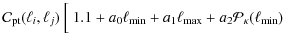
6.3 Accuracy of the fitting formula

To test the performance of the fitting, we calculate the relative deviation between the non-Gaussian covariance computed with the fitting formula and the halo model one. The deviation,

$\begin{displaymath}% \left(\frac{\Delta \mathcal{C}_{ij}}{\mathcal{C}_{ij}}\righ... ...ll_i,\ell_j)}{\mathcal{C}^{\rm NG}_{\rm halo}(\ell_i,\ell_j)}, \end{displaymath}$

(56)

is computed for every wave-number pair $(\ell _i,\ell _j)$ and shown in Fig. 8, for the case of $z_{\rm s}=1$ . The upper left panel of Fig. 8 shows the absolute value of the deviation for each element of the covariance matrix, while the other panels show the deviation along cuts through diagonals of the covariance.

The fit works quite well on the off-diagonal elements that are close to the diagonal, showing an average overestimation of $10\%$ . When moving along any off-diagonal, from larger to smaller scales, (lower panels of Fig. 8), we move from the first fit, Eq. (52), where the deviation is mostly positive, to the second one, Eq. (53), where the deviation is mostly negative. The transition occurs at the local maximum, which indicates that none of the fitting formulae should be extrapolated to the other region. The fits break down on the smallest scales, with the deviation increasing very rapidly when the largest scale reaches $\ell_i \approx 5000$ . Smaller scales would clearly require higher-order terms in Eq. (53).

As we move away from the diagonal the fit gets increasingly worse, in particular the deviations are larger than $100\%$ in the region shown in black in the upper left panel of Fig. 8, which correlates very small with very large scales. The reason for this is that this region was effectively not fitted, since it is not contained in any of the two blocks fitted by Eq. (54). Restricting to the range where both scales are between $50 < \ell < 5000$ , roughly $90\%$ of the elements show deviations between $-25\%$ and $+25\%$ , with the average of the absolute deviations being $10\%$ . This range contains also $9\%$ of outliers where the deviations are larger than ${\pm}25\%$ . The outliers occur in the low-amplitude correlations between the largest $(50 < \ell < 200)$ and smallest $(3000 < \ell < 5000)$ scales.

The fit is worse on the diagonal than on the first off-diagonals (where $\ell_{i}/\ell_{j} < 50$ ). On the diagonal, the fit always underestimates the covariance. Scales in the range $50 < \ell < 5000$ show a deviation between $-40\%$ and $-10\%$ , with an average of $-20\%$ . The accuracy degrades at larger scales, which is not a problem since for $\ell < 50$ the non-Gaussian contribution to the total covariance is negligible, as seen in Fig. 8 (upper right panel). Adding the Gaussian contribution to the fitted non-Gaussian one, the underestimation in the diagonal elements is always better than $10\%$ , with an average of $5\%$ .

In summary, the fitting formula for the cosmic variance, including Gaussian and non-Gaussian contributions, has an average accuracy of $10\%$ in the off-diagonal and $5\%$ in the diagonal. It is valid when both scales are in the range $50 < \ell < 5000$ , corresponding to $2\hbox{$^\prime$ }< \theta < 5^{\circ}$ in real space. This is roughly the range used in the latest results from CFHTLS-Wide (Fu et al. 2008). This range includes the scales where non-Gaussianity is relevant, i.e., where the cosmic shear error budget is both dominated by cosmic variance and has important contributions from non-linear clustering (see Sect. 6.4).

6.4 Impact of the accuracy of the fitting formula on parameter estimations

We study the impact of the fitting formula accuracy on the estimation of cosmological parameters, using a Fisher matrix approach. For this, we need to take into account not only the Gaussian and non-Gaussian contributions to the covariance, but also the noise in the observed power spectrum. In practical applications, the convergence field in Eq. (13) is obtained from the observed ellipticities of the source galaxies. The intrinsic ellipticity field (i.e., in the absence of a gravitational lensing effect) is assumed to have zero mean and rms of $\sigma_\epsilon$ per component. This shape noise contaminates the observed power spectrum. Assuming that the intrinsic ellipticities of different galaxies do not correlate, the shape noise contribution to the covariance of the power spectrum is diagonal and given by the new terms arising in Eq. (14) when replacing the power spectrum, in that expression, by the observed one defined as (Kaiser 1992),

$\begin{displaymath}% P^{\rm obs}_\kappa(\ell)=P_\kappa(\ell)+\frac{\sigma^2_\epsilon}{n}, \end{displaymath}$

(57)

where n is the number density of source galaxies.

We consider the following three surveys: a medium-deep weak lensing survey covering an area of $170~\deg^2$ with $n=10~{\rm arcmin^2}$ , like the current CFHTLS-Wide, a wider survey of similar depth covering $5000~\deg^2$ with $n=10~{\rm arcmin^2}$ , like the planned Dark Energy Survey (DES), and a wide and deep survey with $20~000~\deg^2$ and $n=40~{\rm arcmin^2}$ , like the proposed E UCLID. For all three we assume $\sigma_\epsilon=0.3$ and compute the covariance using the halo model and the developed fit formula in the range $50 < \ell < 5000$ . Additionally, we add the covariance of a Gaussian contribution using a logarithmic binning with 61 bins in a range from $\ell _{\rm low}=1$ to $\ell _{\rm up}=10^5$ . The wider surveys will measure correlations on scales larger than $\ell=50$ , which we do not consider here for comparison purposes. Note also that for very large scales the flat-sky approximation breaks down.

$\begin{figure} \par\hspace*{-2mm}\includegraphics[width=8.1cm,clip]{12854fg14}\vspace*{5mm} \includegraphics[width=7.7cm,clip]{12854fg15} \end{figure}$

Figure 9:

Left panel: relative contributions to the diagonal of the convergence power spectrum covariance. The binning-dependent Gaussian to non-Gaussian ratio (solid line; see caption of Fig. 8 for the employed binning scheme) and the shape noise to cosmic variance ratio for two surveys with $n=10~{\rm arcmin^2}$ and $n=40~{\rm arcmin}^{-2}$ (dotted), are shown as function of multipole $\ell$ . The ticks at the intersection of the $10\%$ line with the ratio curves enclose the approximate range where the non-Gaussian contribution is important for the E UCLID-like survey. Right panel: Fisher ellipses in the $(\Omega _{\rm m},\sigma _8)$ plane ( $2\sigma$ contours) calculated with the halo model covariance (solid) and the fitted covariance (dashed) for the DES-like (large ellipses) and E UCLID-like (small ellipses) surveys. Compared to the halo covariance case, the fitted covariance error ellipses are decreased (enlarged) by $13\%$ ( $10\%$ ) for the DES (E UCLID) case.

Open with DEXTER

The left panel of Fig. 9 compares the different terms contributing to the diagonal of the covariance, by showing the Gaussian to non-Gaussian ratio and the shape noise to cosmic variance ratio, where by cosmic variance we denote the sum of the Gaussian and non-Gaussian contributions. The ratio between the Gaussian and non-Gaussian terms is independent of the survey and, for our particular choice of binning, non-Gaussianity starts to affect the diagonal around $\ell = 300$ , where its amplitude is $10\%$ of the Gaussian amplitude, and dominates from $\ell \approx 1000$ onwards. Shape noise, including both pure shape noise and the coupling with cosmic variance, also becomes important on small scales, but in a survey-dependent way. It is as large as the cosmic variance on $\ell \approx 200$ $(\ell \approx 1000)$ for surveys with 10 (40) galaxies per arcmin squared. The vertical lines in Fig. 9 (left panel) show, for the E UCLID-like survey, the range where the non-Gaussian contribution to the diagonal is non-negligible, i.e., where it accounts for more than $10\%$ of the cosmic variance while having an amplitude of at least $10\%$ of the shape noise. This range is roughly $300 < \ell < 3000$ , or approximately $4 \hbox{$^\prime$ }< \theta < 50 \hbox{$^\prime$ }$ . This is a rough estimate of the minimum range where the fitting formula is required to have a good accuracy.

In addition, the accuracy of the off-diagonal terms is crucial, since the non-Gaussianity is the sole contribution there. To evaluate the required range of validity of the fitting formula, in a way that includes the off-diagonal elements and is independent of bin width, we define the signal-to-noise ratio (Takada & Jain 2009),

$\begin{displaymath}% \left(\frac{S}{N}\right)^2=\sum_{ij}\mathcal{P}_{\kappa}(\ell_i) ~{\mathcal{C}^{-1}_{ij}}~\mathcal{P}_{\kappa}(\ell_j). \end{displaymath}$

(58)

For each survey, we compute the signal-to-noise ratio (SNR) using all scales between $\ell=50$ , the largest scale where the fitting is valid, to successive values of $\ell_{\rm max}$ . The SNR increases with $\ell_{\rm max}$ , as more scales are included in Eq. (58). The increasing rate, however, decreases with increasing $\ell_{\rm max}$ , tending to zero when additional scales do not carry additional cosmological information. The value of $\ell_{\rm max}$ for which this saturation occurs increases with decreasing shape noise, and gives a good indication of the range where the fitting formula is required to have a good accuracy in order to get accurate estimates of cosmological parameters. We find that, when increasing $\ell_{\rm max}$ from $\ell_{\rm {max}}=5000$ to $\ell_{\rm {max}}=10~000$ , the SNR increases by a factor of 1.03 for the CFHTLS-like survey and by a factor of 1.09 for the E UCLID-like survey. Hence, even for the latter there is no much gain in reaching $\ell > 5000$ .

We consider now the Fisher information matrix, which to first order, neglecting the cosmology dependence of the covariance matrix, is given by

$\begin{displaymath}% F_{\alpha\beta}=\sum_{ij}\frac{\partial \mathcal{P}_\kappa(... ...~\frac{\partial \mathcal{P}_\kappa(\ell_j)}{\partial p_\beta}, \end{displaymath}$

(59)

where the derivatives are taken w.r.t. a set of cosmological parameters $p_\alpha$ . The Fisher matrix defines the error ellipsoid in parameter space, with $\left(F^{-1}_{~\alpha\alpha}\right)^{1/2}$ yielding the $1\sigma$ marginalized error on $p_\alpha$ , and $\left(1/F_{\alpha\alpha}\right)^{1/2}$ giving the $1\sigma$ error on $p_\alpha$ assuming the other parameters are perfectly known.

We compute Eq. (59) for both the fit and halo model covariances, for each of the three surveys. We perform the derivatives at the fiducial model of Table 3, varying only 2 cosmological parameters $(\Omega _{\rm m},\sigma _8)$ . For each survey, we compare the areas of the two $2\sigma$ error ellipses (which defines the inverse of the figure-of-merit) thus obtained. For all three cases, there is a good agreement between the two ellipses.

For the two cases with large shape noise, CFHTLS and DES, we find that the fitting formula underestimates the Fisher ellipse, as compared to the halo model covariance. This is expected because with an enhanced diagonal the correlations between bins are weaker, and the result is dominated by the accuracy of the diagonal, where the fitting formula underestimates the covariance, as we saw earlier on. The deviation is however weak, the areas of the ellipses obtained using the fitting formula are $13\%$ smaller than the halo model result, and the deviation is uniformly distributed on the parameter space (see Fig. 9, right panel, large ellipses). This implies that the deviation on the marginalized constraints is much smaller, and we find that the fitting formula underestimates the errors on both $\Omega_{\rm m}$ and $\sigma_8$ by only $1\%$ , for both surveys. This corresponds to a deviation of $0.1\%$ $(0.01\%)$ of the parameters values, for CFHTLS (DES). In contrast, for the E UCLID case, where the covariance has larger correlations, the fitted covariance produced an ellipse slightly larger than the halo model one, by about $10\%$ (see Fig. 9, right panel, small ellipses).

6.5 Covariance of real-space estimators

For practical purposes it is sometimes more convenient to study real-space correlations rather than correlations in Fourier space. We therefore define an estimator of a general second-order cosmic shear measure which is related to the convergence power spectrum estimator by

$\begin{displaymath}% \hat{\Gamma}(\theta)=\int_{0}^{\infty}\frac{{\rm d} \ell~\ell}{2\pi}W(\ell\theta)\hat{P}_{\kappa}(\ell), \end{displaymath}$

(60)

where W(x) is an arbitrary weight function. A well-known example of this equation are the shear two-point correlation functions $\xi_{+}(\theta)$ and $\xi_{-}(\theta)$ with weight functions $W(\ell\theta)={J}_{0}(\ell\theta)$ and $W(\ell\theta)={J}_{4}(\ell\theta)$ , respectively (see discussion in Joachimi et al. 2008). Using the definition Eq. (60), we find for the relation between the covariance of the real-space estimators to the covariance of the Fourier-space estimators:

$\displaystyle % {\rm Cov}\left[\hat{\Gamma}(\theta),\hat{\Gamma}(\theta')\right]$	=	$\displaystyle \int_{0}^{\infty}\frac{{\rm d}\ell~\ell}{2\pi}W(\ell\theta) \int_{0}^{\infty}\frac{{\rm d}\ell'~\ell'}{2\pi}W(\ell'\theta')$
		$\displaystyle \times ~ {\rm Cov}\left[\hat{P}_{\kappa}(\ell),\hat{P}_{\kappa}(\ell')\right],$	(61)

which is related to the covariance of the dimensionless power spectrum used in the fitting formula by $(2\pi)^{2}{\rm Cov}\left[\hat{\mathcal{P}}_{\kappa}(\ell),\hat{\mathcal{P}}_{\k... ...2}\ell'^{2}{\rm Cov}\left[\hat{P}_{\kappa}(\ell),\hat{P}_{\kappa}(\ell')\right]$ . Inserting the result of the dimensionless power spectrum covariance given in Eq. (14) yields

	$\displaystyle {\rm Cov}\left[\hat{\Gamma}(\theta),\hat{\Gamma}(\theta')\right] ... ...rm d}\ell}{\ell^{3}}~\mathcal{P}_{\kappa}^{2}(\ell) W(\ell\theta)W(\ell\theta')$
	$\displaystyle \qquad \qquad+ ~ \frac{1}{A}\int_{0}^{\infty}\frac{{\rm d}\ell}{\... ...\infty}\frac{{\rm d}\ell'}{\ell'}~\bar{T}_{\kappa}(\ell,\ell') W(\ell'\theta').$	(62)

We find that the Gaussian part of the real-space covariance is independent of the binning scheme and is non-diagonal in contrast to the covariance in Fourier space.

7 Conclusions

We present a fitting formula for the halo model prediction of the non-Gaussian contribution to the covariance of the dimensionless power spectrum of the weak lensing convergence. The formula was constructed assuming a ${\Lambda }$ CDM cosmology with WMAP5-like cosmological parameters. In particular, it was obtained for $\Omega_{\rm m}=0.28$ , $\sigma_8=0.82$ and other parameter values as shown in Table 3. It is valid for a scale range of $50 \la \ell \la 5000$ , corresponding to $2'<\theta<5^{\circ}$ in real space and can be used for surveys with galaxy source redshifts $z_{\rm s} \in [0.5,2]$ . In this range, it reproduces the results of a full implementation of the halo model approach, with a scale-averaged accuracy of $10\%$ in the off-diagonal, and $5\%$ in the diagonal elements. The formula also allows us to recover the halo model $(\Omega _{\rm m},\sigma _8)$ error ellipses within $15\%$ . The range of validity of the formula and its level of accuracy render it applicable to low shape noise scenarios from next generation weak lensing surveys.

To use the formula, shown in Eq. (54), one needs three quantities:

The non-Gaussian contribution to the covariance of the convergence power spectrum in tree-level perturbation theory ${\cal C}_{\rm pt}$ , shown in Eq. (A.27). This involves the computation of the convergence trispectrum in tree-level perturbation theory, Eq. (A.26), which requires the calculation of the linear power spectrum and of the F₂ and F₃ coupling functions (Eqs. (A.10) and (A.12)).
The non-linear convergence power spectrum.
The 9 coefficients of the fit, which are obtained by inserting the 27 values given in Table 4 in Eq. (55), for the required redshift.

The Gaussian contribution, calculated from the non-linear convergence power spectrum as given in Eq. (14), may then be added to the result of the formula, to obtain the total covariance. This is the covariance of the estimator without noise, or the cosmic variance.

The work presented in this paper is based on the assumption that the halo model is a powerful approach to probe non-linear clustering. We tried to test this assumption against results from N-body simulations, but our comparisons were inconclusive. Indeed, such analysis requires ray-tracing simulations with both large number of convergence maps and large convergence map area. Only then it would be possible to minimize the effect of sampling variance in the simulations, which hindered our attempted tests. Such simulations would also allow us to consider error bars for the estimate of the simulation covariance. There are however indications that the halo model approach underestimates the non-Gaussianity of the covariance and there are attempts to include additional contributions (Sato et al. 2009; Takada & Jain 2009).

The reliability of the halo model for higher-order polyspectra also needs to be studied in more detail. Some work in this direction are the analyses of the impact of the triaxiality of the halo profiles (Smith et al. 2006; Smith & Watts 2005), and halo exclusion effects (Tinker et al. 2005). Moreover, the issue of halo substructure (Dolney et al. 2004) and of the effect of a stochastic concentration parameter have to be understood properly. This paper also addresses this last issue. We analyze the impact of a stochastic concentration parameter on the covariance of the convergence power spectrum. We found that the effect can safely be neglected for the Gaussian contribution, with the convergence power spectrum varying only slightly, and at small scales, for concentration scatters of $\sigma_{\ln c} \simeq 0.2{-}0.3$ . For the non-Gaussian contribution the effect is more pronounced due to the higher sensitivity of the trispectrum to a stochastic concentration relation. In the case of the 1-halo term of the trispectrum, we find it useful to take into account a concentration dispersion of $\sigma_{\ln c} \ga 0.3$ . The deviation to a deterministic concentration-mass relation is larger than $12\%$ for wave-numbers $\ell \ga 3000$ .

Although the fitting formula we obtained provides a more thorough estimate for the non-Gaussian contribution to the power spectrum covariance than the earlier approximation of Semboloni et al. (2007) (global accuracy of ${\sim}20\%$ along the diagonal, which becomes less for the off-diagonals), there is still room for improvements. One drawback of our approach is that it requires the computation of the convergence trispectrum in tree-level perturbation theory. Furthermore, it is only applicable to a small range of WMAP5-like cosmologies and is only valid in the interval $50 \leq \ell\leq 5000$ . A possible way to avoid these problems and extend the accuracy of the fitting formula might be to construct it entirely from its three-dimensional counterpart, the three-dimensional covariance of the matter power spectrum. This has the advantage that perturbations of different length scales are not additionally mixed due to projection effects, which might allow us to cover a wider range of cosmologies. The desired projected covariance could then be obtained by performing an additional integration along the redshift-space. We will address this issue in a future paper.

Acknowledgements

The authors thank Christoph Lampert for invaluable discussions, and Jan Hartlap for providing his ray-tracing simulations of the Gems and Virgo simulations. Together with Martin Kilbinger both provided useful comments to the manuscript. J.P. would like to thank the TRR33. J.R. is supported by the Deutsche Forschungsgemeinschaft under the project SCHN 342/7-1 within the Priority Programme SPP 1177 ``Galaxy Evolution''. I.T. is supported by the Marie Curie Training and Research Network ``DUEL''.

References

Albrecht, A., Bernstein, G., Cahn, R., et al. 2006 [arXiv:astro-ph/0609591]
Bacon, D. J., Refregier, A. R., & Ellis, R. S. 2000, MNRAS, 318, 625
Bardeen, J. M., Bond, J. R., Kaiser, N., & Szalay, A. S. 1986, ApJ, 304, 15
Bartelmann, M., & Schneider, P. 2001, Phys. Rep., 340, 291
Bernardeau, F., Colombi, S., Gaztañaga, E., & Scoccimarro, R. 2002, Phys. Rep., 367, 1
Bullock, J. S., Kolatt, T. S., Sigad, Y., et al. 2001, MNRAS, 321, 559
Cooray, A., & Hu, W. 2001, ApJ, 554, 56
Cooray, A., & Sheth, R. 2002, Phys. Rep., 372, 1
Dolney, D., Jain, B., & Takada, M. 2004, MNRAS, 352, 1019
Eisenstein, D. J., & Hu, W. 1998, ApJ, 496, 605
Fry, J. N. 1984, ApJ, 279, 499
Fu, L., Semboloni, E., Hoekstra, H., et al. 2008, A&A, 479, 9
Gunn, J. E., & Gott, J. R. I. 1972, ApJ, 176, 1
Hartlap, J., Schrabback, T., Simon, P., & Schneider, P. 2009, A&A, 504, 689
Hilbert, S., Hartlap, J., White, S. D. M., & Schneider, P. 2009, A&A, 499, 31
Hu, W., & Kravtsov, A. V. 2003, ApJ, 584, 702
Jain, B., & Bertschinger, E. 1994, ApJ, 431, 495
Jain, B., Seljak, U., & White, S. 2000, ApJ, 530, 547
Jenkins, A., Frenk, C. S., Pearce, F. R., et al. 1998, ApJ, 499, 20
Jing, Y. P. 2000, ApJ, 535, 30
Joachimi, B., Schneider, P., & Eifler, T. 2008, A&A, 477, 43
Kaiser, N. 1992, ApJ, 388, 272
Kaiser, N. 1998, ApJ, 498, 26
Kaiser, N., Wilson, G., & Luppino, G. A. 2000, unpublished[arXiv:astro-ph/0003338]
Kilbinger, M., & Schneider, P. 2005, A&A, 442, 69
Komatsu, E., Dunkley, J., Nolta, M. R., et al. 2009, ApJS, 180, 330
Ma, C.-P., & Fry, J. N. 2000, ApJ, 543, 503
Massey, R., Heymans, C., Bergé, J., et al. 2007, MNRAS, 376, 13
Nakamura, T. T., & Suto, Y. 1997, Prog. Theor. Phys., 97, 49
Navarro, J. F., Frenk, C. S., & White, S. D. M. 1997, ApJ, 490, 493
Peacock, J. A., & Dodds, S. J. 1996, MNRAS, 280, L19
Peacock, J. A., & Smith, R. E. 2000, MNRAS, 318, 1144
Pielorz, J. 2008, Ph.D. Thesis, University of Bonn
Press, W. H., & Schechter, P. 1974, ApJ, 187, 425
Sato, M., Hamana, T., Takahashi, R., et al. 2009, ApJ, 701, 945
Schäfer, B. M. 2009, Int. J. Modern Phys. D, 18, 173
Schneider, P. 2006, in Gravitational Lensing: Strong, Weak and Micro, Saas-Fee Advanced Courses, ed. P. Schneider, C. S. Kochanek, & J. Wambsganss (Berlin: Springer-Verlag), 33, 269
Schneider, P., van Waerbeke, L., Kilbinger, M., & Mellier, Y. 2002, A&A, 396, 1
Scoccimarro, R., Colombi, S., Fry, J. N., et al. 1998, ApJ, 496, 586
Scoccimarro, R., Sheth, R. K., Hui, L., & Jain, B. 2001, ApJ, 546, 20
Scoccimarro, R., Zaldarriaga, M., & Hui, L. 1999, ApJ, 527, 1
Seljak, U. 2000, MNRAS, 318, 203
Semboloni, E., Tereno, I., van Waerbeke, L., & Heymans, C. 2009, MNRAS, 397, 608
Semboloni, E., van Waerbeke, L., Heymans, C., et al. 2007, MNRAS, 375, L6
Sheth, R. K., & Tormen, G. 1999, MNRAS, 308, 119
Smith, R. E., & Watts, P. I. R. 2005, MNRAS, 360, 203
Smith, R. E., Peacock, J. A., Jenkins, A., et al. 2003, MNRAS, 341, 1311
Smith, R. E., Scoccimarro, R., & Sheth, R. K. 2007, Phys. Rev. D, 75, 063512
Smith, R. E., Watts, P. I. R., & Sheth, R. K. 2006, MNRAS, 365, 214
Springel, V. 2005, MNRAS, 364, 1105
Takada, M., & Jain, B. 2003, MNRAS, 340, 580
Takada, M., & Bridle, S. 2007, New J. Phys., 9, 446
Takada, M., & Jain, B. 2009, MNRAS, 395, 2065
Takahashi, R., Yoshida, N., Takada, M., et al. 2009, ApJ, 700, 479
Tinker, J. L., Weinberg, D. H., Zheng, Z., & Zehavi, I. 2005, ApJ, 631, 41
Van Waerbeke, L., Mellier, Y., Erben, T., et al. 2000, A&A, 358, 30
Vikhlinin, A., Burenin, R. A., Ebeling, H., et al. 2009, ApJ, 692, 1033
Wechsler, R. H., Bullock, J. S., Primack, J. R., Kravtsov, A. V., & Dekel, A. 2002, ApJ, 568, 52
White, M., & Hu, W. 2000, ApJ, 537, 1
Wittman, D. M., Tyson, J. A., Kirkman, D., Dell'Antonio, I., & Bernstein, G. 2000, Nature, 405, 143

Appendix A: Cosmological perturbation theory

On large scales, different Fourier modes evolve independently from each other and thus conserve the Gaussian behavior of the density perturbation field $\tilde{\delta}({\vec k},a)$ . It is therefore convenient to work in Fourier space and Fourier transform the fields as well as the non-linear fluid equations (consisting of continuity, Euler and Poisson equation) that describe their evolution in an expanding Universe. Contrary to linear perturbation theory, there is a coupling between different Fourier modes mediated by the coupling function $\alpha({\vec k}_{1},{\vec k}_{2})$ on smaller scales. In this case, the fluid equations for the density contrast and the irrotational peculiar velocity field $\theta=\nabla\cdot {\vec u}$ in Fourier space are given by (e.g., Bernardeau et al. 2002)

	$\displaystyle a \dot{\tilde{\delta}}({\vec k}, a) + \tilde{\theta}({\vec k},a) ... ...ec k}_1, {\vec k}_2) \tilde{\theta}({\vec k}_1,a) \tilde{\delta}({\vec k}_2,a),$	(A.1)
	$\displaystyle a \dot{\tilde{\theta}}({\vec k},a) + \frac{3H_0^2 \Omega_{\rm m}}... ...vec k}_1,{\vec k}_2) \tilde{\theta}({\vec k}_1,a) \tilde{\theta}({\vec k}_2,a),$	(A.2)

where we introduced the two fundamental mode coupling functions

$\displaystyle % \alpha({\vec k}_{1},{\vec k}_{2})= \frac{({\vec k}_{1}+{\vec k}... ...vert{\vec k_1}+{\vec k_2}\vert^2({\vec k_1}\cdot{\vec k_2})}{2k_1^2 k_2^2}\cdot$

(A.3)

For an Einstein-de Sitter (EdS) cosmology it is possible to find a perturbative ansatz that separates the scale- and time dependencies, whereas for a general ${\Lambda }$ CDM model it is impossible to find a separable solution to Eqs. (A.1) and (A.2). However, Scoccimarro et al. (1998) showed that it is possible to find a separable solution in any order if one makes an approximation that is valid at percentage level. One indeed finds then the same recursion relation as in the EdS case. The ansatz is then

$\begin{displaymath}% \tilde{\delta}({\vec k},a) = \sum_{n=1}^\infty D^n(a)\tild... ... \dot{a} \sum_{n=1}^\infty D^n(a) \tilde{\theta}_n({\vec k}). \end{displaymath}$

(A.4)

Therefore, we find that the whole information on cosmological parameters is encoded in the growth function due to its dependence on the Hubble parameter (see Eq. (5)).

A.1 Coupling functions

The nth order density contrast and the divergence of the peculiar velocity in Eq. (A.4) is given by

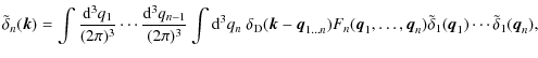
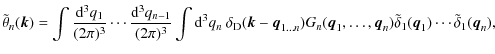
	$\displaystyle \tilde\delta_{n}({\vec k}) = \int \frac{{\rm d}^{3}q_{1}}{(2\pi)^... ...ec q}_{n}) \tilde\delta_{1}({\vec q}_{1})\cdots \tilde\delta_{1}({\vec q}_{n}),$	(A.5)
	$\displaystyle \tilde\theta_{n}({\vec k}) = \int \frac{{\rm d}^{3}q_{1}}{(2\pi)^... ...ec q}_{n}) \tilde\delta_{1}({\vec q}_{1})\cdots \tilde\delta_{1}({\vec q}_{n}),$	(A.6)

and the nth order coupling functions F_n and G_n are obtained by the following recursion relations (Jain & Bertschinger 1994)

	$\displaystyle F_n({\vec q_1},\ldots,{\vec q_n}) = \sum_{m=1}^{n-1} \frac{G_m({\... ..._n}) + 2\beta({\vec k_1},{\vec k_2})G_{n-m}({\vec q_{m+1}},\ldots,{\vec q_n})],$	(A.7)
	$\displaystyle G_n({\vec q_1},\ldots,{\vec q_n}) = \sum_{m=1}^{n-1} \frac{G_m({\... ...n}) + 2n\beta({\vec k_1},{\vec k_2})G_{n-m}({\vec q_{m+1}},\ldots,{\vec q_n})],$	(A.8)

where ${\vec k_1}\equiv {\vec q_1}+\ldots+{\vec q_m}$ and ${\vec k_2}\equiv {\vec q_{m+1}}+\ldots+{\vec q_n}$ . The initial conditions for these recursion relations are $F_1\equiv 1$ and $G_1\equiv 1$ . To get the functions $F_n^{({\rm s})}$ and $G_n^{({\rm s})}$ that are symmetric in its arguments, one must perform the following symmetrizing procedure

$\displaystyle % F_n^{(\textrm{s})}({\vec q_1},\ldots,{\vec q_n})= \frac{1}{n!}\... ...ec q_n})= \frac{1}{n!}\sum_\pi G_n({\vec q_{\pi(1)}},\ldots,{\vec q_{\pi(n)}}),$

(A.9)

where the sum is taken over all possible permutations $\pi$ of the set $\{ 1,\ldots,n\}$ . These equations enable us to calculate the density contrast in the nth order of perturbation theory by using the iterative equations for the coupling functions.

The calculation of the second-order coupling functions is straightforward. The result is

$\displaystyle % F_2^{(\textrm{s})}({\vec q_1},{\vec q_2}) = \frac{5}{7}+ \frac{... ...q_1}\cdot{\vec q_2}}{q_1 q_2} \left(\frac{q_1}{q_2}+\frac{q_2}{q_1}\right)\cdot$

(A.10)

The third-order coupling function is given by

$\displaystyle % F_3({\vec q_1},{\vec q_2},{\vec q_3}) = \frac{1}{18}\Big\{ 7\al... ...vec q_3}) + 2\beta({\vec q}_{12},{\vec q_3})] G_2({\vec q_1},{\vec q_2})\Big\},$

(A.11)

where ${\vec q}_{ij}\equiv {\vec q}_{i}+{\vec q}_{j}$ . Employing Eq. (A.9), we find the symmetric function

$\displaystyle % F_3^{(\textrm{s})}({\vec q_1},{\vec q_2},{\vec q_3})$	=	$\displaystyle \frac{7}{54} [\alpha({\vec q_1},{\vec q}_{23})F_2^{(\textrm{s})}(... ...3}) +\alpha({\vec q_3},{\vec q}_{12})F_2^{(\textrm{s})}({\vec q_1},{\vec q_2})]$
		$\displaystyle + ~ \frac{4}{54} [\beta({\vec q_1},{\vec q}_{23})G_2^{(\textrm{s}... ..._3}) +\beta({\vec q_3},{\vec q}_{12})G_2^{(\textrm{s})}({\vec q_1},{\vec q_2})]$
		$\displaystyle + ~\frac{7}{54} [\alpha({\vec q}_{12},{\vec q_3})G_2^{(\textrm{s}... ...}) +\alpha({\vec q}_{23},{\vec q_1})G_2^{(\textrm{s})}({\vec q_2},{\vec q_3})].$	(A.12)

From now on the symmetry superscript `` (s)'' will be omitted because we will only deal with symmetric coupling functions. For the calculation of the trispectrum in the halo model approach as described in Sect. 4.5, one needs perturbation theory. More precisely, we need the subsequent components

$\displaystyle % F_3({\vec q_1},-{\vec q_1},{\vec q_2})$	=	$\displaystyle \frac{7}{54} [\alpha({\vec q_1},{\vec q}_{-})F_2(-{\vec q_1},{\vec q_2})+ \alpha(-{\vec q_1},{\vec q}_{+})F_2({\vec q_1},{\vec q_2})]$
		$\displaystyle + ~ \frac{4}{54} [\beta({\vec q_1},{\vec q}_{-})G_2(-{\vec q_1},{\vec q_2})+ \beta(-{\vec q_1},{\vec q}_{+})G_2({\vec q_1},{\vec q_2})]$
		$\displaystyle + ~\frac{7}{54} [\alpha({\vec q}_{-},{\vec q_1})G_2(-{\vec q_1},{\vec q_2})+ \alpha({\vec q}_{+},-{\vec q_1})G_2({\vec q_1},{\vec q_2})],$	(A.13)

where we have defined the difference vector ${\vec q}_{-}\equiv {\vec q}_{2}-{\vec q}_{1}$ and the sum of the vectors ${\vec q}_{+}\equiv {\vec q}_{1}+{\vec q}_{2}$ .

We already mentioned in the previous section that it is possible to find a solution for an arbitrary cosmology if one makes a small approximation. In the literature one can find closed solutions for the second- and third-order coupling functions. The second-order coupling function changes to

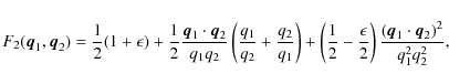
$\begin{displaymath}% F_{2}({\vec q}_{1},{\vec q}_{2})=\frac{1}{2}(1+\epsilon)+\f... ...frac{({\vec q}_{1}\cdot{\vec q}_{2})^{2}}{q_{1}^{2}q_{2}^{2}}, \end{displaymath}$

(A.14)

where $\epsilon\approx (3/7)\Omega_{\rm m}^{-2/63}$ for $\Omega_{\rm m}\ga 0.1$ (Bernardeau et al. 2002). For our fiducial choice of $\Omega_{\rm m}=0.3$ , we get $\Omega_{\rm m}^{-2/63}\approx 1.039$ . Thus, within a few percent correction to the first and last term, the coupling functions are independent of cosmological parameters.

A.2 Correlation functions

A.2.1 Bispectrum

The dark matter bispectrum is defined as

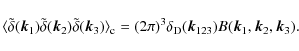
$\begin{displaymath}% \langle \tilde\delta({\vec k}_{1}) \tilde\delta({\vec k}_{2... ... D}({\vec k}_{123}) B({\vec k}_{1},{\vec k}_{2},{\vec k}_{3}). \end{displaymath}$

(A.15)

Since the connected bispectrum vanishes for Gaussian random fields, it is the first intrinsically non-linear moment. Inserting the perturbative expansion (A.4) for each term results generally in an infinitely large sequence of correlators. The lowest non-vanishing order is the so-called tree-level contribution to the bispectrum. We find for the correlator in tree level

$\displaystyle % \langle \tilde\delta({\vec k}_{1})\tilde\delta({\vec k}_{2}) \t... ...ec k}_{1})\tilde\delta_{1}({\vec k}_{2}) \tilde\delta_{2}({\vec k}_{3})\rangle.$

(A.16)

Replacing the second-order density contrast with Eq. (A.5) results in

$\displaystyle % \langle\tilde\delta_{2}({\vec k}_{1})\tilde\delta_{1}({\vec k}_{2})\tilde\delta_{1}({\vec k}_{3})\rangle$	=	$\displaystyle \int\frac{{\rm d}^{3}q_{1}}{(2\pi)^3}\int{\rm d}^{3}q_{2}~ \delta... ...\vec q}_{2})\tilde\delta_{1}({\vec k}_{2})\tilde\delta_{1}({\vec k}_{3})\rangle$
	=	$\displaystyle (2\pi)^{3}\delta_{\rm D}({\vec k}_{123}) ~ 2F_{2}({\vec k}_{2},{\vec k}_{3})P_{\rm {lin}}(k_{2})P_{\rm {lin}}(k_{3}),$	(A.17)

where we applied Wick's theorem to express the four-point correlator of Gaussian fields in terms of products of power spectra, and performed the two integrations over the Dirac delta distributions. The results for the other two terms of the tree-level bispectrum are simply obtained by permutations of the arguments. Finally, the tree-level bispectrum is given by

$\displaystyle % B_{\rm {pt}}({\vec k}_{1},{\vec k}_{2},{\vec k}_{3})= 2F_{2}({\... ...c k}_{1},{\vec k}_{3})P_{1}P_{3} + 2F_{2}({\vec k}_{2},{\vec k}_{3})P_{2}P_{3}.$

(A.18)

The factor 2 follows from using the symmetrized version of the second-order coupling function.

A.2.2 Trispectrum

The dark matter trispectrum is defined as the connected four-point function in Fourier space:

$\begin{displaymath}% \langle \tilde\delta({\vec k}_{1}) \tilde\delta({\vec k}_{2... ...234}) T({\vec k}_{1},{\vec k}_{2},{\vec k}_{3},{\vec k}_{4}), \end{displaymath}$

(A.19)

where ${\vec k}_{1234}\equiv {\vec k}_{1}+{\vec k}_{2}+{\vec k}_{3}+{\vec k}_{4}$ . We find that there are two different non-vanishing contributions to the tree level:

$\displaystyle % \langle \tilde\delta({\vec k}_{1}) \tilde\delta({\vec k}_{2})\tilde\delta({\vec k}_{3})\tilde\delta({\vec k}_{4}) \rangle_{\rm tree}$	=	$\displaystyle \langle \tilde\delta_{2}({\vec k}_{1}) \tilde\delta_{2}({\vec k}_... ...{\vec k}_{3})\tilde\delta_{1}({\vec k}_{4}) \rangle + \ldots (\textrm{6~terms})$
		$\displaystyle + ~ \langle \tilde\delta_{3}({\vec k}_{1}) \tilde\delta_{1}({\vec... ...\vec k}_{3}) \tilde\delta_{1}({\vec k}_{4}) \rangle +\ldots (\textrm{4~terms}).$	(A.20)

In total we find 6 terms of the first type and 4 terms for the second type, where the rest is obtained by permutations. All other contributions either vanish or are built of higher-order terms. Note that for the second type of terms we need the results from perturbation theory up to the third order. The calculation of each term is a tedious but straightforward calculation. We obtain for the first term of the expansion

$\displaystyle % \langle \tilde\delta_{2}({\vec k}_{1}) \tilde\delta_{2}({\vec k... ...)+ P_{14}F_{2}({\vec k}_{3},-{\vec k}_{23})F_{2}({\vec k}_{4},-{\vec k}_{14})],$

(A.21)

where the six-point correlator resolves into 15 terms consisting of power spectra products. Performing the integrations over the arising delta functions yields in the end 8 different terms. Similarly, we find for the second type of terms

$\displaystyle % \langle \tilde\delta_{3}({\vec k}_{1}) \tilde\delta_{1}({\vec k... ...vec k}_{1234}) ~ 6F_{3}({\vec k}_{2},{\vec k}_{3},{\vec k}_{4})P_{2}P_{3}P_{4}.$

(A.22)

The other terms are easily obtained by permutations, however, we present here the complete result to avoid confusion with a shorthand notation that is introduced afterwards. The trispectrum of cold dark matter is in first non-vanishing order given by (Fry 1984):

$\begin{displaymath}% T_{\rm {pt}} = 4 T_a+ 6 T_b, \end{displaymath}$

(A.23)

where

T_a	=	$\displaystyle P_1 P_2 \left[ P_{13} F_2({\vec k}_1,-{\vec k}_{13}) F_2({\vec k}... ...) + P_{14} F_2({\vec k}_1,-{\vec k}_{14}) F_2({\vec k}_2,{\vec k}_{14}) \right]$
		$\displaystyle + ~ P_1 P_3 \left[ P_{12} F_2({\vec k}_1,-{\vec k}_{12}) F_2({\ve... ...) + P_{14} F_2({\vec k}_1,-{\vec k}_{14}) F_2({\vec k}_3,{\vec k}_{14}) \right]$
		$\displaystyle + ~ P_1 P_4 \left[ P_{12} F_2({\vec k}_1,-{\vec k}_{12}) F_2({\ve... ...) + P_{13} F_2({\vec k}_1,-{\vec k}_{13}) F_2({\vec k}_4,{\vec k}_{13}) \right]$
		$\displaystyle + ~ P_2 P_3 \left[ P_{21} F_2({\vec k}_2,-{\vec k}_{21}) F_2({\ve... ...) + P_{24} F_2({\vec k}_2,-{\vec k}_{24}) F_2({\vec k}_3,{\vec k}_{24}) \right]$
		$\displaystyle + ~ P_2 P_4 \left[ P_{21} F_2({\vec k}_2,-{\vec k}_{21}) F_2({\ve... ...) + P_{23} F_2({\vec k}_2,-{\vec k}_{23}) F_2({\vec k}_4,{\vec k}_{23}) \right]$
		$\displaystyle + ~ P_3 P_4 \left[ P_{31} F_2({\vec k}_3,-{\vec k}_{31}) F_2({\ve... ... + P_{32} F_2({\vec k}_3,-{\vec k}_{32}) F_2({\vec k}_4,{\vec k}_{32}) \right],$	(A.24)

and

$\displaystyle % T_b = F_3({\vec k}_1,{\vec k}_2,{\vec k}_3) P_1 P_2 P_3 + F_3({... ..._4,{\vec k}_1) P_3 P_4 P_1 + F_3({\vec k}_4,{\vec k}_1,{\vec k}_2) P_4 P_1 P_2,$

(A.25)

where $P_{i}\equiv P_{\rm {lin}}(k_{i})$ , $P_{ij}\equiv P_{\rm {lin}}(\vert{\vec k}_{i}+{\vec k}_{j}\vert)$ and ${\vec k}_{ij}\equiv {\vec k}_{i}+{\vec k}_{j}$ .

For the covariance matrix one only needs the parallelogram configuration. This imposes the condition ${\vec k}_{2}=-{\vec k}_{1}$ and ${\vec k}_{4}=-{\vec k}_{3}$ on the wave-vectors. In this case Eq. (A.23) simplifies to

$\displaystyle % T_{\rm {pt}}$	=	$\displaystyle 4 P_{1}^{2} \left\{ [F_2({\vec k_1},-{\vec k}_{+})]^2 P_{+}\right... ...+})]^2 P_{+} \right. + \left. [F_2({\vec k_3},- {\vec k}_{-})]^2 P_{-} \right\}$
		$\displaystyle + ~ 8 P_{1} P_{3} \left[F_2({\vec k_1},-{\vec k}_{+}) F_2({\vec k... ...P_{+} + F_2({\vec k_1},{\vec k}_{-}) F_2({\vec k_3},-{\vec k}_{-}) P_{-}\right]$
		$\displaystyle + ~ 12 \left[P_1^2 P_3 F_3({\vec k_1},-{\vec k_1},{\vec k_3}) + P_1 P_3^{2} F_3({\vec k_1},{\vec k_3},-{\vec k_3})\right],$	(A.26)

where ${\vec k}_{-}\equiv{\vec k}_{3}-{\vec k}_{1}$ , ${\vec k}_{+}\equiv{\vec k}_{1}+{\vec k}_{3}$ , $P_{-}\equiv P_{\rm {lin}}(\vert{\vec k}_{-}\vert)$ and $P_{+}\equiv P_{\rm {lin}}(\vert{\vec k}_{+}\vert)$ . Consequently, we define the non-Gaussian contribution to the covariance in tree-level perturbation theory as

$\begin{displaymath}% {\cal C}_{\rm pt} \equiv {\cal C}_{\rm pt}(\ell_{i},\ell_{j... ...{w},\frac{{\vec \ell}_2}{w},-\frac{{\vec \ell}_2}{w},w\right), \end{displaymath}$

(A.27)

where A denotes the survey area, $A_{\rm {r}}(\ell)$ the integration area and G(w) the lensing weight function (see Eq. (7)). More details on the notation can be found in Sect. 3.

Footnotes

... theory: We refer by tree-level perturbation theory to the lowest, non-vanishing order of the considered quantity in perturbation theory.
... Transform: For the FFT we use an algorithm from the GNU scientific library (see http://www.gnu.org/software/gsl/ for more details).
... spectrum: Using the hierarchical ansatz, which is approximately valid in the highly nonlinear regime, the three-dimensional dark matter trispectrum is proportional to the power spectrum cubed.
... (DES): http://www.darkenergysurvey.org/
... UCLID: http://www.dune-mission.net/

All Tables

Table 1: Cosmological parameters used to set up the initial power spectrum.

Table 2: Parameters used for generating the two N-body simulations.

Table 3: Fiducial model used for the fitting procedure.

Table 4: Best-fit values for the parameters (p₀,p₁,p₂) of the redshift-fit for the set of coefficients $(a_0,\ldots,a_8)$ .

All Figures

$\begin{figure} \par\includegraphics[width=12cm,clip]{12854fg1} \end{figure}$	Figure 1: Square configuration of the dimensionless convergence trispectrum ${\cal T}^n_\kappa (\ell )$ against wave-number $\ell$ for the range $10 \leq \ell \leq 10^4$ for $n \in \{\mbox{1h, 2h, 3h, 4h, tot, pt}\}$ . The upper panel displays the four individual halo terms, the sum of all four trispectrum halo terms ${\cal T}^{\rm tot}_\kappa$ (solid line) and the tree-level perturbation theory trispectrum ${\cal T}^{\rm pt}_\kappa$ , as indicated in the key. The lower panel shows the ratio between the indicated contributions and the complete trispectrum. The double dashed line illustrates the corresponding ratio of the approximation ${\cal T}^{\rm tot}_\kappa \approx {\cal T}^{\rm pt}_\kappa + {\cal T}^{\rm 1h}_\kappa$ . Note that we consider the 4-halo term only in the upper panel since it resembles the term ${\cal T}^{\rm pt}_\kappa$ on large scales.
Open with DEXTER
In the text

$\begin{figure} \par\includegraphics[width=12cm,clip]{12854fg2} \end{figure}$	Figure 2: Contour plots of the ratio $R(\ell _i,\ell _j)$ between the non-Gaussian covariance 1-halo term contribution (see Eq. (48)) computed with a concentration dispersion $\sigma_{\ln c}$ and with a deterministic concentration, against wave-numbers $(\ell _i,\ell _j)$ ranging from $\ell _i=\ell _j=500$ to $\ell _i=\ell _j=8500$ . The left panel is for concentration dispersion $\sigma_{\ln c}=0.15$ , whereas in the right panel $\sigma_{\ln c}=0.3$ .
Open with DEXTER
In the text

$\begin{figure} \par\hspace{0.25mm}\includegraphics[width=11.9cm,clip]{12854fg3}... ...e{0.25mm}\vspace*{3mm} \includegraphics[width=12cm,clip]{12854fg4} \end{figure}$	Figure 3: Dimensionless convergence power spectrum ${\cal P}_\kappa (\ell )$ against wave-number $\ell$ for galaxy sources at redshift $z_{\rm s}=1$ ( upper panels) and $z_{\rm s}=2$ ( lower panels). Points with error bars show measurements from the two sets of numerical simulations: Gems (left plots) and Virgo (right plots). Both simulations use a similar particle setup but differ in the area of the $\kappa$ -maps (see Tables 1 and 2). They are compared with the corresponding results obtained with fitting formulae from Smith et al. (long-dashed line), Peacock-Dodds (short-dashed line), and the halo model predictions for a deterministic halo concentration (solid line). See text for a discussion.
Open with DEXTER
In the text

$\begin{figure} \par\includegraphics[width=15cm,clip]{12854fg5} \end{figure}$	Figure 4: Relative difference $\Delta \mathcal{C}_{ij}/\mathcal{C}_{ij}$ (see Eq. (51)) between the halo model prediction for the covariance of the convergence power spectrum and the results from the Virgo simulation ( $z_{\rm s}=1$ ) against wave-numbers $(\ell _i,\ell _j)$ . The binning scheme is linear with a constant bin width of $\Delta l=720$ ranging from $\ell _0=720$ to $\ell _{20}=15120$ . The left panel displays the full covariance, including all four halo terms for the trispectrum, and uses a deterministic concentration-mass relation denoted by $\sigma_{\ln c}=0$ . The right panel illustrates the same covariance but with a stochastic concentration distribution of width $\sigma_{\ln c}=0.3$ for the 1-halo term of the trispectrum.
Open with DEXTER
In the text

$\begin{figure} \par\includegraphics[width=15cm,clip]{12854fg6} \end{figure}$	Figure 5: Relative difference $\Delta \mathcal{C}_{ij}/\mathcal{C}_{ij}$ (see Eq. (51)) between the halo model prediction for the covariance of the convergence power spectrum and the results from the Gems simulation ( $z_{\rm s}=1$ ) against wave-numbers $(\ell _i,\ell _j)$ . The binning scheme is linear with a constant bin width of $\Delta l=90$ ranging from $\ell _0=90$ to $\ell _{20}=7020$ . The left panel displays the full covariance, including all four halo terms for the trispectrum, and uses a deterministic concentration-mass relation denoted by $\sigma_{\ln c}=0$ . The right panel illustrates the same covariance but with a stochastic concentration distribution of width $\sigma_{\ln c}=0.3$ for the 1-halo term of the trispectrum.
Open with DEXTER
In the text

$\begin{figure} \par\includegraphics[width=9cm,clip]{12854fg7} \end{figure}$	Figure 6: Ratio ${\cal C}_{\rm pt}/{\cal C}^{\rm NG}$ against wave-numbers $(\ell _i,\ell _j)$ . The covariance in tree-level perturbation theory resembles the non-Gaussian covariance on very large scales (i.e., $\ell _i=\ell _j\leq 20$ ) to approximately $80{-}90\%$ except along the diagonal and the closest off-diagonals. Here a good approximation of the non-Gaussian covariance requires at least one additional halo term. For wave-numbers $\ell _i=\ell _j\geq 100$ , an accurate description of the non-Gaussian covariance requires at least the 1-halo term.
Open with DEXTER
In the text

$\begin{figure} \par\includegraphics[width=8.5cm,clip]{12854fg8}\vspace*{2mm} \includegraphics[width=8.5cm,clip]{12854fg9} \end{figure}$	Figure 7: Coefficients a_i of the fitting formula obtained for various source redshifts. Left (right) panel shows the coefficients of the large (small) scales fitting formula. For convenience, scaled versions of the coefficients are shown, as indicated in the key. Note for example that a₅, a₇ and a₈ change sign. The lines show the redshift fit, Eq. (55), with the parameters given in Table 4. They provide a good fit for $z_{\rm s}>0.5$ (indicated by the vertical line).
Open with DEXTER
In the text

$\begin{figure} \par\mbox{\includegraphics[angle=0,width=8.5cm]{12854fg10}\includ... ....5cm]{12854fg12}\includegraphics[angle=0,width=8.5cm]{12854fg13} }\end{figure}$	Figure 8: Accuracy of the fitting formula for $z_{\rm s}=1$ . Upper left panel: relative deviation $\Delta \mathcal{C}_{ij}/\mathcal{C}_{ij}$ , defined in Eq. (56). Other panels: diagonal cuts through the fitted non-Gaussian covariance, showing the covariance on the diagonal $\ell _{i}=\ell _{j}$ ( upper-right panel), for $\ell _i = 4.6 \ell _j$ ( lower-left) and for $\ell _i = 10 \ell _j$ ( lower-right). All three panels show the fitted and the halo model non-Gaussian covariances (as well as the Gaussian for the upper-right panel) as function of the lowest scale $\ell _j$ in the upper part, and the deviation in percent in the lower part, where the dashed lines mark the $25\%$ level. For the Gaussian covariance we employed a logarithmic binning with 61 bins in a range from $\ell _{\rm low}=1$ to $\ell _{\rm up}=10^5$ .
Open with DEXTER
In the text

$\begin{figure} \par\hspace{-2mm}\includegraphics[width=8.1cm,clip]{12854fg14}\vspace{5mm} \includegraphics[width=7.7cm,clip]{12854fg15} \end{figure}$	Figure 9: Left panel: relative contributions to the diagonal of the convergence power spectrum covariance. The binning-dependent Gaussian to non-Gaussian ratio (solid line; see caption of Fig. 8 for the employed binning scheme) and the shape noise to cosmic variance ratio for two surveys with $n=10~{\rm arcmin^2}$ and $n=40~{\rm arcmin}^{-2}$ (dotted), are shown as function of multipole $\ell$ . The ticks at the intersection of the $10\%$ line with the ratio curves enclose the approximate range where the non-Gaussian contribution is important for the E UCLID-like survey. Right panel: Fisher ellipses in the $(\Omega _{\rm m},\sigma _8)$ plane ( $2\sigma$ contours) calculated with the halo model covariance (solid) and the fitted covariance (dashed) for the DES-like (large ellipses) and E UCLID-like (small ellipses) surveys. Compared to the halo covariance case, the fitted covariance error ellipses are decreased (enlarged) by $13\%$ ( $10\%$ ) for the DES (E UCLID) case.
Open with DEXTER
In the text

Current usage metrics show cumulative count of Article Views (full-text article views including HTML views, PDF and ePub downloads, according to the available data) and Abstracts Views on Vision4Press platform.

Data correspond to usage on the plateform after 2015. The current usage metrics is available 48-96 hours after online publication and is updated daily on week days.

Initial download of the metrics may take a while.

A fitting formula for the non-Gaussian contribution to the lensing power spectrum covariance

1 Introduction

2 Structure formation in a CDM cosmology

3 Covariance of the convergence power spectrum

4 Halo model

4.1 Overview

4.2 Ingredients

4.3 Building blocks

4.4 Power spectrum

4.5 Trispectrum

4.6 Convergence spectra

4.7 Stochastic halo concentration

5 Comparison with N-body simulations

5.1 Virgo and Gems simulation

5.2 Ray-tracing

5.3 Convergence power spectrum

5.4 Covariance of the convergence power spectrum

6 Fitting formula for the covariance of the convergence power spectrum

6.1 Methodology

6.2 Redshift dependence

6.3 Accuracy of the fitting formula

6.4 Impact of the accuracy of the fitting formula on parameter estimations

6.5 Covariance of real-space estimators

7 Conclusions

References

Appendix A: Cosmological perturbation theory

A.1 Coupling functions

A.2 Correlation functions

A.2.1 Bispectrum

A.2.2 Trispectrum

Footnotes

All Tables

All Figures

2 Structure formation in a ${\Lambda }$ CDM cosmology