The instability transition for the restricted 3-body problem

J. Eberle; M. Cuntz

doi:10.1051/0004-6361/200912500

Home

All issues

Volume 514 (May 2010)

A&A, 514 (2010) A19

Full HTML

Free Access

Issue		A&A Volume 514, May 2010


Article Number		A19
Number of page(s)		8
Section		Celestial mechanics and astrometry
DOI		https://doi.org/10.1051/0004-6361/200912500
Published online		04 May 2010

A&A 514, A19 (2010)

II. The hodograph eccentricity criterion

J. Eberle¹ - M. Cuntz^1,2

1 - Department of Physics, Science Hall, University of Texas at Arlington, Arlington, TX 76019-0059, USA
2 - Institut für Theoretische Astrophysik, Universität Heidelberg, Albert Überle Str. 2, 69120 Heidelberg, Germany

Received 14 May 2009 / Accepted 20 January 2010

Abstract
Aims. We present a new method that allows identifying the onset of orbital instability, as well as quasi-periodicity and multi-periodicity, for planets in binary systems. This method is given for the special case of the circular restricted 3-body problem (CR3BP).
Methods. Our method relies on an approach given by differential geometry that analyzes the curvature of the planetary orbit in the synodic coordinate system. The centerpiece of the method consists in inspecting the effective (instantaneous) eccentricity of the orbit based on the hodograph in rotated coordinates and in calculating the mean and median values of the eccentricity distribution.
Results. Orbital stability and instability can be mapped by numerically inspecting the hodograph and/or the effective eccentricity of the orbit in the synodic coordinate system. The behavior of the system depends solely on the mass ratio $\mu$ of the binary components and the initial distance ratio $\rho _0$ of the planet relative to the stellar separation distance noting that the stellar components move on circular orbits. Our study indicates that orbital instability occurs when the median of the effective eccentricity distribution exceeds unity. This instability criterion can be compared to other criteria, including those based on Jacobi's integral and the zero-velocity contour of the planetary orbit.
Conclusions. The method can be used during detailed numerical simulations and in contrast to other methods such as methods based on the Lyapunov exponent does not require a piece-wise secondary integration of the planetary orbit. Although the method has been deduced for the CR3BP, it is likely that it can be expanded to more general cases.

Key words: binaries: general - celestial mechanics - planetary systems

1 Introduction

In the past few years the study of planets in stellar binary systems has reached a heightened level of intensity owing to significant new developments in both observations and theory (e.g., Jones 2008). Observations have shown that planets are able to exist in relatively close binary systems with separation distances of 20 to 25 AU, a result presented by Patience et al. (2002), Eggenberger et al. (2004), and Eggenberger & Udry (2007). In addition, theoretical simulations have been done on planet formation in binary systems, which have led to highly favorable outcomes; see, e.g., Kley (2001), Quintana et al. (2002), and subsequent studies. This type of research is also motivated by the ongoing quest to find new extra-solar planets and to analyze their orbital stability, noting that stellar binary systems occur in high frequency in the local Galactic neighborhood (Raghavan et al. 2006; Duquennoy & Mayor 1991; Lada 2006).

Another important aspect pertinent to planets in binary systems, the focus of this paper, is orbital stability. In previous work, we investigated the stability of both S-type and P-type orbits in stellar binary systems and deduced orbital stability limits for planets (Musielak et al. 2005). P-type orbits lie well outside the binary system, where the planet essentially orbits the center of mass of both stars, whereas S-type orbits lie near one of the stars, with the second star exerting perturbational influence. The limits of stability were found to depend on the mass ratio between the stellar components. Earlier results for S-type orbits were given by, e.g., Holman & Wiegert (1999), who considered orbital simulations for various eccentricities of the binary components, and deduced appropriate fitting formulas for the limits of orbital stability. For circular orbits, the Holman & Wiegert stability limit is similar to the one identified by Musielak et al. (2005).

The circular restricted 3-body problem (CR3BP) is a well-established topic of celestial mechanics (Szebehely 1967; Roy 2005, and references therein). The CR3BP describes the motion of a body of negligible mass moving in the gravitational field of the two massive primaries. The primaries move on circular orbits around their center of mass and their motion is not influenced by the third body, the planet. Additionally, the initial velocity of the planet is usually also assumed in the same direction as the orbital velocity of its host star, which is typically the more massive of the two stars. Research results have also been given for more general orbital problems, including the elliptical restricted 3-body problem (ER3BP), which has been studied by Dvorak (1984), Dvorak (1986), Rabl & Dvorak (1988), and more recently by Pilat-Lohinger & Dvorak (2002) and Szenkovits & Makó (2008). Both Dvorak (1986) and Pilat-Lohinger & Dvorak (2002) investigated the stability domain for S-type orbits, whereas Szenkovits & Makó (2008) presented a sophisticated analytical study.

In the case of the CR3BP, the stability limits previously obtained have recently been updated by Cuntz et al. (2007) and (Eberle et al. 2008, Paper I) based on an analytical approach. Cuntz et al. and Eberle et al. were able to derive a stringent (sufficient) criterion for orbital stability based on Jacobi's constant and Jacobi's integral, akin to the criterion of ``Hill stability''. It was found that the planetary orbital stability was guaranteed only if its initial starting position is below a well-defined limit $\rho_0^{(1)}$ , which can also be found by inspecting the ``zero-velocity contour'' in the synodic coordinate system. The orbital stability of a planet is ensured if the zero-velocity contour is closed around the star it orbits, which limits the allowable region of the planet as dictated by its available kinetic energy.

It is noteworthy that the property of the planet to remain within the zero-velocity contour is obviously tantamount to orbital stability, although it does not necessarily imply stability in the sense of quasi-periodicity. In fact, Eberle et al. (2008) encountered evidence that quasi-periodic orbits may even occur for planets outside the previously established stability region. This is a sincere motivation to revisit the onset of orbital instability by assessing the potential of different types of approaches. Our methodology for the study of orbital instability is discussed in Sect. 2. Detailed model simulations are given in Sect. 3, and our conclusions are presented in Sect. 4.

2 Theoretical approach

2.1 Basic equations

Following Paper I, we consider a binary system with the mass M=M₁+M₂, where M₁ and M₂ are the masses of the primary and secondary star, respectively. The mass of the planet is assumed to be very small (``negligible mass'') compared to the stellar masses and the two stars are assumed to orbit each other in circular orbits (CR3BP); see, e.g., Szebehely (1967) and Roy (2005). The distance of the planet to star i = 1, 2 is given as r_i(t)noting that X₃(t) and Y₃(t) are the (sidereal) coordinates of the planet with t as time. The distance D between the binary stars can be used as a scale factor to normalize distances using X₃ = Dx₃ and Y₃ = Dy₃. Thus, the dimensionless position vector for the planetary mass in the sidereal reference frame is given as (x₃, y₃). Similar to Paper I, the dimensionless time $\tau$ is defined as $\tau = {\omega}t$ where $\omega$ denotes the angular frequency of the motion of the binary components.

The dimensionless representation of the velocity and acceleration for the planet is given as ${{\rm d}{X_3}/{{\rm d}t}} = D{\omega}\dot{x}_3$ and ${{\rm d}^2{X_3}/{{\rm d}t^2}} = D{\omega}^2\ddot{x}_3$ , respectively. Equivalent equations hold for the variables in the y direction. By introducing $\mu = {M_2 / M}$ and $\alpha = 1-\mu$ , equations for $\ddot{x}_3$ and $\ddot{y}_3$ can be deduced with

$\displaystyle r_1(t) = \left[(x_3(t)-\mu\cos{\tau})^2+(y_3(t)-\mu\sin{\tau})^2\right]^{1\over 2}$
		(1)
$\displaystyle r_2(t) = \left[(x_3(t)+\alpha\cos{\tau})^2+(y_3(t)+\alpha\sin{\tau})^2\right]^{1\over 2} .$

Next we introduce a synodic coordinate system where we use an asterisk (*) for distinction. We also introduce a scalar pseudo-potential given as

$\begin{displaymath}\overline{\phi} = {1\over 2} \left[\left({x^*_3}^2+{y^*_3}^2\right)+2\left({\alpha \over r_1}+{\mu\over r_2}\right)\right] \end{displaymath}$

(2)

that is connected to the velocity of the planet v^* via

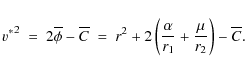
$\begin{displaymath}{v^*}^2 \ = \ 2\overline{\phi} - \overline{C} \ = \ {r}^2+2\left({\alpha \over r_1}+{\mu\over r_2}\right)-\overline{C} . \end{displaymath}$

(3)

This is an integral of motion in the rotating Cartesian coordinate system known as Jacobi's integral (see Paper I and references therein). The constant $\overline{C}$ can be set by the system parameters $\mu$ and $\alpha$ , noting that $\alpha = 1-\mu$ , as well as the initial conditions. It is also connected to the Jacobi constant C via $C = \overline{C} + \mu(1-\mu)$ .

The system parameters $\mu$ and $\alpha$ and the initial conditions, allowing v^*₀ to be set, can also be used to formulate an expression for the Jacobi constant C, which is

$\begin{displaymath} C \ = \ 2\left[\alpha\left({{{\rho_0}^3+2}\over {2\rho_0}} \... ...ft({(1+\rho_0)^3+2}\over {2(1+\rho_0)}\right)\right]-{v^*_0}^2 \end{displaymath}$

(4)

where $\rho _0$ is the planet's relative initial distance as and v^*₀ is the planet's initial velocity. If v^*₀ is set as $\sqrt{(1-\mu)/\rho_0}-\rho_0$ , corresponding to an initially circular orbit concerning the planet, the Jacobi constant can also be expressed as

$\begin{displaymath}C \ = \ \mu+2\mu\rho_0+{{1-\mu}\over\rho_0}+{2\mu\over{1+\rho_0}}+2\sqrt{\rho_0(1-\mu)} . \end{displaymath}$

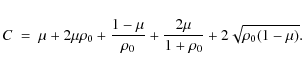
(5)

Obviously, the Jacobi constant depends solely on the parameters $\mu$ and $\rho _0$ of the star-planet system and, furthermore, will not change with time. As discussed in Paper I, as well as previously available literature, Eq. (5) can be used to define absolute limits of stability as well as zero-velocity curve (contour) that form the boundaries of regions where the planet must be found. The rationale of the contour is that it limits the allowable region of the planet defined by its available energy.

2.2 Introduction of the effective eccentricity

Sir William Rowan Hamilton is credited with the notion of the hodograph as a way of describing a planetary orbit based on the variation of the velocity vector (see Hamilton 1847). Simply put, the hodograph is the path that the tip of the velocity vector traces out as it varies about the fixed origin. In particular, Hamilton showed that under the influence of the central inverse square gravitational force, the hodograph is always a circle. For a more recent and accessible discussion see, e.g., Butikov (2000).

We consider polar coordinates by starting from the familiar form of the Kepler orbit

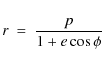
$\begin{displaymath}r \ = \ {p\over{1+e\cos{\phi}}} \end{displaymath}$

(6)

where $\phi = \theta - \theta_0$ . Here r denotes the radius, ethe eccentricity, p the semi-latus rectum, and $\phi$ and $\theta$ denote angles with $\theta_0$ indicating the initial value and measured from the +x axis.

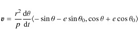
In Cartesian vector form, we find $\vec{r} = \langle r\cos{\theta},r\sin{\theta}\rangle$ . Now, we differentiate with respect to time to obtain the velocity vector $\vec{v} = \langle v_x,v_y\rangle$ , which can be found with simple algebra as

$\begin{displaymath}\vec{v} = {r^2\over{p}}{{\rm d}\theta\over{{\rm d}t}}\langle... ...in{\theta}-e\sin{\theta_0},\cos{\theta}+e\cos{\theta_0}\rangle \end{displaymath}$

(7)

and can be expressed in two parts $\vec{v} = \vec{Q} + \vec{O}$ , noting that

$\displaystyle \vec{Q}$	=	$\displaystyle {h\over p}\langle-\sin{\theta},\cos{\theta}\rangle$	(8)
$\displaystyle \vec{O}$	=	$\displaystyle {he\over p}\langle-\sin{\theta_0},\cos{\theta_0}\rangle ,$	(9)

where $\vec{Q}$ is the rotating component and $\vec{O}$ is the constant center. In the latter transformation, we made use of the identity $r^2{{{\rm d}\theta}/{{\rm d}t}} = {L/m} = h$ indicating the conservation of angular momentum, denoted as L, where h is sometimes referred to as specific angular momentum. It is also assumed that the mass of the planet m does not change during the planetary orbital motion.

The velocity vector constitutes a vector of constant length $Q=\vert\vec{Q}\vert={h/p}$ rotating about a center located at $\vec{O}$ , where $O=\vert\vec{O}\vert={{he}/p}$ . To find a more appropriate representation, we consider the velocity axes rotated $90^\circ$ clockwise from the position axes. In this case, the hodograph will be traced out in the same manner as the orbit, e.g., if the orbit is counterclockwise, then the hodograph will be traced out counterclockwise as well. Moreover, the length and position of the velocity vector allow us to identify the effective eccentricity (i.e., locally defined along-side the hodograph), as we find e = O/Q.

For a Keplerian orbit, the situation is as follows: If e<1 then we have a closed elliptical orbit and the origin of the coordinate system lies within the circle; in the special case of e=0, we have a circular orbit and the center in velocity space coincides with the origin. If e=1, we have a parabolic orbit and the circular hodograph passes through the origin in velocity space. If e>1, the orbit is hyperbolic and the origin in velocity space lies outside the perimeter of the hodograph.

For a non-Kepler orbit, as obtained in conjunction with the restricted three body problem, it is again possible to determine at any given moment the eccentricity from the radius of curvature and the center of curvature of the hodograph. The radius of curvature of a parameterized function such as x = f(t) and y = g(t) can be obtained as

$\begin{displaymath}Q \ = \ {1\over{A}}\big({{\dot{f}}^2+{\dot{g}}^2}\big)^{3/2} \end{displaymath}$

(10)

whereas the location of the center of curvature $(\xi,\eta)$ is given as

$\displaystyle \xi \ = \ f-{1\over{A}}\big({{\dot{f}}^2+{\dot{g}}^2}\big)\dot{g}$		(11)
$\displaystyle \eta \ = \ g+{1\over{A}}\big({{\dot{f}}^2+{\dot{g}}^2}\big)\dot{f}$		(12)

with A=|A'| and

$\begin{displaymath}A' \ = \ \left\vert \begin{array}{c c} \dot{f} & \dot{g} \\ \ddot{f} & \ddot{g}\\ \end{array}\right\vert \end{displaymath}$

(13)

(see, e.g., Bronshtein & Semendyayev 1997). The distance of the center of curvature from the origin can thus be obtained as $O = \sqrt{{\xi}^2+{\eta}^2}$ . For the restricted three body problem, we take f(t) = V_y^* and g(t) = -V_x^* with the asterisk denoting the usage of the synodic (rotating) coordinate system. Therefore, the effective eccentricity at any instant is given as e^* = O(t)/Q(t)(see Fig. 1).

$\begin{figure} \par\includegraphics[width=7cm,clip]{12500fig1.eps} \end{figure}$	Figure 1: Two examples of a circle of curvature for a hodograph depicting the motion of a planet in the synodic coordinate system ( V_y^,V_x^).
Open with DEXTER

3 Results and discussion

$\begin{figure} \par\includegraphics[width=4.5cm,clip]{12500fig21.eps}\hspace{4m... ...ps}\hspace{4mm} \includegraphics[width=4.5cm,clip]{12500fig24.eps} \end{figure}$	Figure 2: Case studies for the initial planetary distance ratios $\rho _0 = 0.40$ , 0.474, 0.50, and 0.595 with the planetary orbits displayed in the synodic coordinate system. The stellar mass ratio is $\mu = 0.3$ .
Open with DEXTER

$\begin{figure} \par\includegraphics[width=4.5cm,clip]{12500fig31.eps}\hspace{4m... ...ps}\hspace{4mm} \includegraphics[width=4.5cm,clip]{12500fig34.eps} \end{figure}$	Figure 3: Same as Fig. 2, but now the case studies are represented by the behavior of the hodograph.
Open with DEXTER

$\begin{figure} \par\includegraphics[width=4.5cm,clip]{12500fig41.eps}\hspace{4m... ...par\vspace{2mm} \includegraphics[width=4.5cm,clip]{12500fig43.eps} \end{figure}$	Figure 4: Same as Fig. 2, but now the case studies are represented by the behavior of the effective eccentricity projected onto the unit velocity vector, except for the model of $\rho _0 = 0.595$ .
Open with DEXTER

$\begin{figure} \par\includegraphics[width=12cm,clip]{12500fig5.eps} \vspace*{2mm} \end{figure}$	Figure 5: Effective eccentricity projected onto the unit velocity vector for the case study $\rho _0 = 0.595$ .
Open with DEXTER

$\begin{figure} \par\includegraphics[width=4.5cm,clip]{12500fig61.eps}\hspace{4m... ...ps}\hspace{4mm} \includegraphics[width=4.5cm,clip]{12500fig64.eps} \end{figure}$	Figure 6: Case studies for the initial planetary distance ratios $\rho _0 = 0.29$ , 0.37, 0.40, and 0.43 with the planetary orbits displayed in the synodic coordinate system. The stellar mass ratio is $\mu = 0.5$ .
Open with DEXTER

$\begin{figure} \par\includegraphics[width=4.5cm,clip]{12500fig71.eps}\hspace{4m... ...ps}\hspace{4mm} \includegraphics[width=4.5cm,clip]{12500fig74.eps} \end{figure}$	Figure 7: Same as Fig. 6, but now the case studies are represented by the behavior of the hodograph.
Open with DEXTER

$\begin{figure} \par\includegraphics[width=4.5cm,clip]{12500fig81.eps}\hspace{4m... ...ps}\hspace{4mm} \includegraphics[width=4.5cm,clip]{12500fig84.eps} \end{figure}$	Figure 8: Same as Fig. 6, but now the case studies are represented by the behavior of the effective eccentricity projected onto the unit velocity vector.
Open with DEXTER

In the following, we consider the CR3BP (Szebehely 1967; Roy 2005, and references therein). For our study, we assume that the planetary mass is $1 \times 10^{-6}$ of the mass of the star it orbits. Additionally, we assume that the initial velocity of the planet is in the same direction as the orbital velocity of its host star, which is the more massive of the two stars, and that the starting position of the planet is to the right of the primary star along the line joining the binary components (3 o'clock position). Obviously, the planetary mass deviates from a zero test mass. Nevertheless, it is not expected to have a significant effect on the motion of the two stars, implying that the conclusions derived from the CR3BP concept remain valid.

We performed simulations for stellar mass ratios from $\mu = 0.0$ to $\mu = 0.5$ in increments of 0.01. As a measure of the precision of the integration scheme, we note that a time step of $\epsilon = 10^{-4}$ yrs is used as it has been carefully tested by inspecting the orbital paths under a variety of initial conditions based on time steps of $\epsilon = 10^{-5}$ and 10^-6 yrs with no discernable difference. We also set an upper time limit of 10³ yrs for our simulations. Although this value is very small, it is sufficient for models of orbital stability if the stability can be proven analytically (Eberle et al. 2008; Cuntz et al. 2007), or for determining and evaluating orbital instability if the planet is ejected from the system or captured by the secondary star prior to the pre-set time of simulation. Surely, there is no guarantee that the orbit of a potentially unstable planet that appears stable over the time of integration will remain stable beyond the allotted time as this would require longer simulations.

$\begin{figure} \par\includegraphics[width=8.5cm,clip]{12500fig9cmjn.eps} \end{figure}$

Figure 9:

We depict the median effective eccentricity (color coded) for various mass ratios $\mu$ and initial conditions $\rho _0$ . The crosses are cases where the simulation was terminated due to the planet captured by one of the stars or being ejected from the system. The twelve white spots are cases where the planet was ejected from the system less ``severely'' and the simulation was not halted. The green, red, and black curves represent the initial conditions which cause the ZVC to intersect L₁, L₂, and L₃, respectively. The pink diamonds are limits of stability given by Pilat-Lohinger & Dvorak (2002).

Open with DEXTER

We display runs for selected initial conditions (i.e., starting distances $\rho _0$ of the planet from the stellar primary) corresponding to $\mu = 0.3$ in Figs. 2 to 5 and to $\mu = 0.5$ in Figs. 6 to 8. In Figs. 2 and 6, we present the planetary orbits in the synodic coordinate system (X^*,Y^*). In Figs. 3 and 7, the same simulations are depicted by using the hodograph (V_y^*,-V_x^*) and in Figs. 4, 5 and 8 by using the effective eccentricity (e_x^*,e_y^*) projected onto the unit velocity vector. The selected starting distance ratios $\rho _0$ of the planet are 0.40, 0.474, 0.50, and 0.595 for $\mu = 0.3$ and 0.29, 0.37, 0.40, 0.43 for $\mu = 0.5$ . Note that $\rho _0$ indicates the relative initial distance of the planet, given as R₀/D, with D = 1 AU as the distance between the two stars and R₀ as the initial distance of the planet from its host star, the primary star of the binary system.

As this system has been studied before, both analytically and numerically, we have solid information on the conditions for planetary orbital stability. Absolute orbital stability occurs if $\rho_0 < \rho_0^{(1)}$ where $\rho_0^{(1)}$ represents the point at which the initial conditions result in a zero-velocity contour that intersects L₁. For larger values of $\rho _0$ , stability is not guaranteed, because the zero-velocity contour opens at the Lagrange points L₁, L₂, and L₃ for $\rho_0^{(1)}$ , $\rho_0^{(2)}$ , and $\rho_0^{(3)}$ , which for $\mu = 0.3$ are given as 0.311, 0.404, and 0.593, and for $\mu = 0.5$ are given as 0.251, 0.442, and 0.442, respectively (e.g., Eberle et al. 2008; Cuntz et al. 2007). Note that for $\mu = 0.5$ the zero-velocity contour opens at L₂ and L₃ simultaneously for obvious reasons. Any such opening, in principle, allows the planet to be captured by the secondary star or to escape from the system entirely.

However, in certain cases this may not happen after all. Eberle et al. (2008) identified a domain of quasi-periodic orbital stability, embedded in the domain of instability in the ( $\rho_0,\mu$ ) diagram. A key example studied here is $\mu = 0.3$ and $\rho_0 = 0.474$ , where the orbit and hodograph show periodic behavior (see Figs. 2 and 3). The orbital data indicate that the planet crosses the X^* axis every quarter of the binary period. The planet's orbit starts at the right outermost position (i.e., 0.474 AU from the primary star), then continues on to the innermost crossing on the left. After another quarter period the planet is crossing on the innermost path on the right. The rest of the orbit follows as outermost left, innermost right again, then innermost left again and then finally after a total of one and a half times the binary period the planet returns to where it started and the orbital pattern repeats.

The corresponding hodograph (Fig. 3) shows an equivalent behavior except that at distances further away from the primary star slower velocities are generally attained and vice versa. There is no indication of planetary escape at all, although no firm statement can be made about the long-term nature of the orbit. Note that the effective eccentricity if projected onto the unit velocity vector also traces out a periodic pattern (see Fig. 4). Moreover, the point at which the effective eccentricity is at its largest, the planet is passing closest to the L₁ point. The eccentricity distribution indicates a mean value of 0.82 and a median value of 0.75 (with a standard deviation of $\sigma_e = 0.35$ ; see Table 1), consistent with the previous interpretation. Note that the case of $\rho_0 = 0.4$ also shows quasi-stability, but there is no quasi-periodicity obtained for the planetary orbit.

A different situation occurs for $\rho_0 = 0.5$ and 0.595. In these cases, no multi-periodicity if found, and the hodograph shows a highly complex topology. Additionally, larger values for the median values of the eccentricity distribution are attained, which are 0.85 and 1.14, respectively. However, even though the model $\rho_0 = 0.5$ should correspond to an unstable orbit, as previously pointed out, no evidence of planetary escape surfaces. This situation is very different for $\rho _0 = 0.595$ , a case where the planet escapes from the system after nearly 211 yrs. This outcome is also reflected by the extreme behavior of the eccentricity vector (e_x^*,e_y^*) (see Fig. 5), exhibiting values beyond 6.3 and 1.4 for e_x^* and e_y^*, respectively.

A further analysis shows that the transition of the median in the eccentricity distribution beyond unity occurs at about $\rho_0 = 0.58$ , which is surprisingly close to $\rho_0 = \rho_0^{(3)}$ , where the zero-velocity contour is open at all Lagrange points L₁, L₂, and L₃. For the sake of curiosity, we also pursued simulations with relatively close planetary starting positions $\rho _0$ , which were 0.2 and 0.3 (see Table 1). In both cases, orbital stability is guaranteed because of the stringent stability criterion, attained for $\rho_0 < \rho_0^{(1)}$ with $\rho_0^{(1)} = 0.311$ . This result is also supported by analyses invoking histograms of the eccentricity distributions which again reveal the mean and median values of the effective eccentricity during the onset of planetary orbital instability.

The development of instability as $\rho _0$ increases is different for $\mu = 0.5$ . The zero-velocity contour opens up at L₁ for $\rho_0 = 0.251$ ; therefore, unstable orbits occur for smaller $\rho _0$ values as expected. For $\rho _0 = 0.29$ the planetary orbit is just on the verge of being unstable as it is slowly spiraling away from the primary star and toward the secondary star (see Fig. 6). For slightly larger $\rho _0$ values, the planet spirals away quickly and transfers to the secondary star and possibly back again before it crashes into one of the stars. For $\rho _0$ between 0.38 and 0.42 there appears to be a quasi-stable region; note that $\rho_0 = 0.4$ is particularly interesting because it seems to correspond to a periodic case. The upper limit of this quasi-stable region corresponds to $\rho _0$ where the zero-velocity contour close to the L₂ and L₃ points opens up and the planetary orbits once again exhibit instability.

Table 1: Effective eccentricity study for the models of $\mu = 0.3$ .

If the planet orbits close to the primary star, the effective eccentricity remains low for the entire duration of the simulation. When the parameters are such that the zero-velocity contour is nearly intersecting the L₁ equilibrium point (C₁ contour, green in Fig. 9), the effective eccentricity increases. For mass ratios less than 0.1 the zero-velocity contour corresponding to L₂ (C₂, red in Fig. 9) is a suitable limit for instability. For initial conditions where the planet is far enough away that the zero-velocity curve as already opened up at L₃ (C₃ contour, black in Fig. 9), the planet is insufficiently bound to be able to orbit the primary star. Therefore, it quickly escapes from the region of the binary stars and for most initial conditions, the planet quickly returns and rapidly approaches one of the stars.

In Fig. 9 we show the median effective eccentricity over the 1000 year time period for all $\mu$ and $\rho _0$ that we considered in our simulations. The white regions with black crosses represent simulations that were terminated before the maximum 1000 year limit due to captures by one of the stars or ejection from the system. One unstable region is in the upper mass ratio range, roughly from $\mu = 0.35$ to 0.50 and another is from 0.00 to 0.23. Between these two regions ( $\mu = 0.24$ to 0.34) there is a quasi-stable region in which the effective eccentricity increases almost uniformly. The boundaries of this region remain basically the same for the duration of the simulation as obtained by the inspection of the median effective eccentricity over the course of the binary period. Of course, we should not be surprised if the quasi-stable region were to shrink over a longer time period as 1000 orbits is not a very long time when considering long term stability. In fact, there is already an instability ``island chain'' slowly forming right in the middle of this quasi-stable region. The reasons for this instability ``archipelago'' are still under investigation.

As a comparison to other work, we show the minimum and maximum extension of the stable zone for the circular case taken from Pilat-Lohinger & Dvorak (2002) as pink diamonds. These limits were determined by setting various initial conditions for the third body such that it would have various initial eccentricities and then using the Fast Lyapunov Indicator method (Froeschlé et al. 1997) to determine the extents for which the orbit was unstable. This work conveys the minimum and maximum stable extensions of the stable zones, which apparently group around the C₁ curve associated with the stringent limit of stability given by the CR3BP.

Table 2: Effective eccentricity study for the models of $\mu = 0.5$ .

4 Conclusion

We present a new method that allows identifying the onset of orbital instability for planets in binary systems. The method can be used ``along the way'' of detailed numerical simulations, and does not require a piece-wise secondary integration as, e.g., methods based on the Lyapunov exponent. Thus, it is an alternative to other methods such as, e.g., the Fast Lyapunov Indicator method (Fouchard et al. 2002) as it allows important insight into the properties of dynamic systems such as quasi-periodicity and multi-periodicity of orbits (as gauged by the hodograph), besides the identification of the onset of orbital instability. If a planet becomes orbitally unstable, high effective eccentricities are attained, which facilitates the new criterion. When the planet has left the system, it typically moves in a slowly expanding spiral if viewed in the synodic coordinate system corresponding to an effective eccentricity of close to zero. In this case, our criterion has become defunct, and if needed should be replaced by an assessment of the semimajor axis of the planet, which is expected to reach relatively high values.

Our method relies on a differential geometrical approach that analyzes the curvature of the planetary orbit in the synodic coordinate system. Based on our simulations, it is found that when the median of the eccentricity distribution exceeds unity, orbital instability occurs. This criterion can be included in detailed simulations in an automated mode allowing the identification of planetary ejection in a straightforward manner. Intuitively, this criterion also agrees with the most basic property of conic sections representing closed orbits for e < 1 and open orbits for $e \ge 1$ , although it utilizes a modified definition of eccentricity.

A comparison with the zero-velocity contour of the planetary orbit shows that this criterion, which is a sufficient criterion for orbital instability, closely coincides with the opening of the zero-velocity contour at the Lagrange point L₃, located to the right of the primary star, as previously discussed by Cuntz et al. (2007) and Eberle et al. (2008). If instability occurs, extremely large effective eccentricities are found, indicating a highly hyperbolic planetary orbit in the synodic coordinate system, a stark indication of planetary escape. Although our results have been described for the special case of the CR3BP, we expect that it may also be possible to augment this criterion to planets in generalized stellar binary systems, and to used it for the assessment of long-term simulations. Clearly, the CR3BP is an idealized case which is barely (if at all) realized in nature. Desired generalizations should include studies of the ER3BP (e.g., Pilat-Lohinger & Dvorak 2002; Szenkovits & Makó 2008) as well as of planets on inclined orbits (Dvorak et al. 2007), noting that especially the former have important applications to real existing systems in consideration of the identified stellar and planetary orbital parameters (Eggenberger & Udry 2007).

Acknowledgements

This work has been supported by the Department of Physics, University of Texas at Arlington.

References

Bronshtein, I. N., & Semendyayev, K. A. 1997, Handbook of Mathematics, 3rd edn (New York: Springer)
Butikov, E. I. 2000, Eur. J. Phys., 21, 297
Cuntz, M., Eberle, J., & Musielak, Z. E. 2007, ApJ, 669, L105
Duquennoy, A., & Mayor, M. 1991, A&A, 248, 485
Dvorak, R. 1984, Celest. Mech. Dyn. Astron., 34, 369
Dvorak, R. 1986, A&A, 167, 379
Dvorak, R., Schwarz, R., Suli, Á., & Kotoulas, T. 2007, MNRAS, 382, 1324
Eberle, J., Cuntz, M., & Musielak, Z. E. 2008, A&A, 489, 1329 (Paper I)
Eggenberger, A., & Udry, S. 2007, in Planets in Binary Star Systems, ed. N. Haghighipour (New York: Springer), in press [arXiv:0705.3173]
Eggenberger, A., Udry, S., & Mayor, M. 2004, A&A, 417, 353
Fouchard, M., Lega, E., Froeschlé, Ch., & Froeschlé, Cl. 2002, Celest. Mech. Dyn. Astron., 83, 205
Froeschlé, C., Lega, E., & Gonczi, R. 1997, Celest. Mech. Dyn. Astron., 67, 41
Hamilton, W. R. 1847, in Proc. Royal Irish Academy, ed. D. R. Wilkins 3, 344
Holman, M. J., & Wiegert, P. A. 1999, AJ, 117, 621
Jones, B. W. 2008, Int. J. Astrobiol., 7, 279
Kley, W. 2001, in The Formation of Binary Stars, ed. H. Zinnecker, & R. D. Mathieu (San Francisco: ASP), IAU Symp., 200, 511
Lada, C. J. 2006, ApJ, 640, L63
Musielak, Z. E., Cuntz, M., Marshall, E. A., & Stuit, T. D. 2005, A&A, 434, 355; Erratum, 480, 573, 2008
Patience, J., White, R. J., Ghez, A. M., et al. 2002, ApJ, 581, 654
Pilat-Lohinger, E., & Dvorak, R. 2002, Celest. Mech. Dyn. Astron., 82, 143
Quintana, E. V., Lissauer, J. J., Chambers, J. E., & Duncan, M. J. 2002, ApJ, 576, 982
Rabl, G., & Dvorak, R. 1988, A&A, 191, 385
Raghavan, D., Henry, T. J., Mason, B. D., et al. 2006, ApJ, 646, 523
Roy, A. E. 2005, Orbital Motion (Bristol and Philadelphia: Institute of Physics Publ.)
Szebehely, V. 1967, Theory of Orbits (New York and London: Academic Press)
Szenkovits, F., & Makó, Z. 2008, Celest. Mech. Dyn. Astron., 101, 273

Footnotes

... negligible: Negligible mass means that although the body's motion is influenced by the gravity of the two massive primaries, its mass is too low to affect the motions of the primaries.
... with: Note that Eq. (1) also corrects a typo in Eq. (6) of Paper I.
... 344: see http://www.maths.soton.ac.uk/EMIS/classics/Hamilton/Hodo.pdf

All Tables

Table 1: Effective eccentricity study for the models of $\mu = 0.3$ .

Table 2: Effective eccentricity study for the models of $\mu = 0.5$ .

All Figures

$\begin{figure} \par\includegraphics[width=7cm,clip]{12500fig1.eps} \end{figure}$	Figure 1: Two examples of a circle of curvature for a hodograph depicting the motion of a planet in the synodic coordinate system ( V_y^,V_x^).
Open with DEXTER
In the text

$\begin{figure} \par\includegraphics[width=4.5cm,clip]{12500fig21.eps}\hspace{4m... ...ps}\hspace{4mm} \includegraphics[width=4.5cm,clip]{12500fig24.eps} \end{figure}$	Figure 2: Case studies for the initial planetary distance ratios $\rho _0 = 0.40$ , 0.474, 0.50, and 0.595 with the planetary orbits displayed in the synodic coordinate system. The stellar mass ratio is $\mu = 0.3$ .
Open with DEXTER
In the text

$\begin{figure} \par\includegraphics[width=4.5cm,clip]{12500fig31.eps}\hspace{4m... ...ps}\hspace{4mm} \includegraphics[width=4.5cm,clip]{12500fig34.eps} \end{figure}$	Figure 3: Same as Fig. 2, but now the case studies are represented by the behavior of the hodograph.
Open with DEXTER
In the text

$\begin{figure} \par\includegraphics[width=4.5cm,clip]{12500fig41.eps}\hspace{4m... ...par\vspace{2mm} \includegraphics[width=4.5cm,clip]{12500fig43.eps} \end{figure}$	Figure 4: Same as Fig. 2, but now the case studies are represented by the behavior of the effective eccentricity projected onto the unit velocity vector, except for the model of $\rho _0 = 0.595$ .
Open with DEXTER
In the text

$\begin{figure} \par\includegraphics[width=12cm,clip]{12500fig5.eps} \vspace*{2mm} \end{figure}$	Figure 5: Effective eccentricity projected onto the unit velocity vector for the case study $\rho _0 = 0.595$ .
Open with DEXTER
In the text

$\begin{figure} \par\includegraphics[width=4.5cm,clip]{12500fig61.eps}\hspace{4m... ...ps}\hspace{4mm} \includegraphics[width=4.5cm,clip]{12500fig64.eps} \end{figure}$	Figure 6: Case studies for the initial planetary distance ratios $\rho _0 = 0.29$ , 0.37, 0.40, and 0.43 with the planetary orbits displayed in the synodic coordinate system. The stellar mass ratio is $\mu = 0.5$ .
Open with DEXTER
In the text

$\begin{figure} \par\includegraphics[width=4.5cm,clip]{12500fig71.eps}\hspace{4m... ...ps}\hspace{4mm} \includegraphics[width=4.5cm,clip]{12500fig74.eps} \end{figure}$	Figure 7: Same as Fig. 6, but now the case studies are represented by the behavior of the hodograph.
Open with DEXTER
In the text

$\begin{figure} \par\includegraphics[width=4.5cm,clip]{12500fig81.eps}\hspace{4m... ...ps}\hspace{4mm} \includegraphics[width=4.5cm,clip]{12500fig84.eps} \end{figure}$	Figure 8: Same as Fig. 6, but now the case studies are represented by the behavior of the effective eccentricity projected onto the unit velocity vector.
Open with DEXTER
In the text

$\begin{figure} \par\includegraphics[width=8.5cm,clip]{12500fig9cmjn.eps} \end{figure}$	Figure 9: We depict the median effective eccentricity (color coded) for various mass ratios $\mu$ and initial conditions $\rho _0$ . The crosses are cases where the simulation was terminated due to the planet captured by one of the stars or being ejected from the system. The twelve white spots are cases where the planet was ejected from the system less ``severely'' and the simulation was not halted. The green, red, and black curves represent the initial conditions which cause the ZVC to intersect L₁, L₂, and L₃, respectively. The pink diamonds are limits of stability given by Pilat-Lohinger & Dvorak (2002).
Open with DEXTER
In the text

Current usage metrics show cumulative count of Article Views (full-text article views including HTML views, PDF and ePub downloads, according to the available data) and Abstracts Views on Vision4Press platform.

Data correspond to usage on the plateform after 2015. The current usage metrics is available 48-96 hours after online publication and is updated daily on week days.

Initial download of the metrics may take a while.