| Issue |
A&A
Volume 513, April 2010
|
|
|---|---|---|
| Article Number | L1 | |
| Number of page(s) | 4 | |
| Section | Letters | |
| DOI | https://doi.org/10.1051/0004-6361/201014294 | |
| Published online | 14 April 2010 | |
LETTER TO THE EDITOR
Nonaxisymmetric modes of MRI in dissipative Keplerian disks
L. L. Kitchatinov1,2,3 - G. Rüdiger1
1 - Astrophysikalisches Institut Potsdam, An der Sternwarte 16,
14482 Potsdam, Germany
2 -
Institute for Solar-Terrestrial Physics, PO Box
291, Irkutsk 664033, Russia
3 -
Pulkovo Astronomical Observatory, St. Petersburg 196140, Russia
Received 19 February 2010 / Accepted 17 March 2010
Abstract
Aims. Deviations from the axial symmetry are necessary to
maintain self-sustained MRI-turbulence by a dynamo mechanism. We define
the parameter region where the nonaxisymmetric MRI modes are excited
and study their geometries and growth rates.
Methods. The linear eigenvalue problem for global
nonaxisymmetric modes of standard-MRI in Keplerian disks is solved
numerically with allowance for finite diffusion.
Results. For small magnetic Prandtl numbers the microscopic
viscosity completely drops out of the analysis so that the stability
maps and the growth rates expressed in terms of the magnetic Reynolds
number Rm and the Lundquist number S do not depend on the magnetic
Prandtl number Pm. The minimum magnetic field for the onset of
nonaxisymmetric MRI grows with the rotation rate. For a given S all
nonaxisymmetric modes disappear for a sufficiently large Rm. This is a
consequence of the radial fine-structure of the nonaxisymmetric modes
resulting from the winding effect of differential rotation. It is this
fine-structure which also provides serious resolution problems for the
numerical simulation of MRI at large Rm.
Conclusions. For weak magnetic fields slightly above the
critical value for the onset of MRI only axisymmetric modes are
unstable. Nonaxisymmetric modes need stronger fields and not too large
Rm. If Pm is small its real value does not play any role in MRI.
Key words: instabilities - magnetohydrodynamics (MHD) - magnetic fields - accretion, accretion disks
1 Introduction
Currently the leading mechanism for the origin of turbulence in accretion disks is the magnetorotational instability (MRI). The instability can be excited by even a very weak magnetic field provided that there is a rotation with outward decreasing angular velocity (see Balbus & Hawley 1998).
The MRI is expected to possess the remarkable property of being self-sustained, i.e. to support the destabilizing magnetic field via its own dynamo (Brandenburg et al. 1995; Hawley et al. 1996). Deviations from the axial symmetry are necessary for any dynamo (Cowling 1933; Elsasser 1946) which in this case have to be produced by the MRI itself. An excitation of nonaxisymmetric modes of MRI is thus necessary for the self-sustained turbulence.
The present paper focuses on the nonaxisymmetric modes of the MRI. A
model of a Keplerian disk with finite diffusivities and an axial
background field is used in a linear analysis of global stability.
As in the axisymmetric case, the nonaxisymmetric MRI exists in a
range between some minimum
![]() and maximum
and maximum
![]() values of the background field. The instability
range depends on the rotation rate (parameterized by the magnetic
Reynolds number
values of the background field. The instability
range depends on the rotation rate (parameterized by the magnetic
Reynolds number ![]() ). In contrast to the axisymmetric case,
however, the
). In contrast to the axisymmetric case,
however, the
![]() for nonaxisymmetric modes does not
approach a (low) constant value for an increasing rotation rate, but
grows with
for nonaxisymmetric modes does not
approach a (low) constant value for an increasing rotation rate, but
grows with ![]() .
The larger the
.
The larger the ![]() ,
therefore, the
stronger is the axial field required to maintain the nonaxisymmetric
instability.
,
therefore, the
stronger is the axial field required to maintain the nonaxisymmetric
instability.
This behavior is extremely difficult to follow numerically because
of the winding effect of differential rotation. The shearing
of nonaxisymmetric fields by differential rotation produces radial
fine structures when the field is too weak to resist the winding.
This shearing effect must be the reason for the increase of
![]() with
with ![]() and also for the high resolution
required to resolve the nonaxisymmetric MRI numerically (see Fromang
& Papaloizou 2007).
and also for the high resolution
required to resolve the nonaxisymmetric MRI numerically (see Fromang
& Papaloizou 2007).
2 The model
The model of Kitchatinov & Mazur (1997) of a rotating disk
of constant thickness, 2H, threaded by a uniform axial magnetic
field is used. The rotation axis is normal to the disk plane and the
angular velocity, ![]() ,
varies only with the distance s to the
axis, i.e.
,
varies only with the distance s to the
axis, i.e.
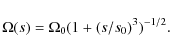
This profile describes an almost uniform rotation with the angular velocity
where

The equations are linearized about the basic state of rotational motion (1) and uniform axial magnetic field

with
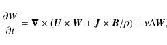
The magnetic and velocity disturbances are expressed in terms of
scalar potentials, e.g.
so that the disturbances are automatically divergence-free. Then Fourier expansions in z and in the azimuthal coordinate
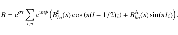
are applied. The summation in (6) runs over l = 1,2,3,...and m=0,1,2,... The mathematical treatment of the velocity and vorticity disturbances is quite similar.
The equation system for the disturbances splits into a set of independent equations for different l and m. It is also important that the terms marked by the upper indexes S and A in (6) are not mixed by the equations. These indexes mark the magnetic modes symmetric and antisymmetric relative to the midplane of the disk. We shall use the notation Sm and Am for the symmetric and antisymmetric modes where m is the azimuthal wave number. Note that Sm and Am represent families of modes that can be further distinguished by the vertical wave number l. For a fixed m, l, and a given symmetry type we have an eigenvalue problem for ordinary differential equations in the variable y, which is solved numerically.
The problem has three governing parameters, i.e. the ![]() ,
the Lundquist number (
,
the Lundquist number (![]() )
and
the magnetic Prandtl number (
)
and
the magnetic Prandtl number (![]() )
)
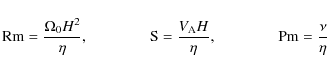
with
3 Local analysis for axisymmetric modes
For disturbances of a small spatial scale compared to the local radius
the differential rotation can be approximated by a plane-shear flow
which leads to the local approximation (Hawley & Balbus
1991). For the simplest case of plane-wave disturbances with
![]() one finds the dispersion relation
one finds the dispersion relation

where

(Kitchatinov & Rüdiger 2004). The dimensionless quantities (7) have been redefined in terms of the wave number (
Equation (9) shows that the instability requires sufficiently
large ![]() exceeding
exceeding
![]() corresponding to
corresponding to
![]() .
For
.
For
![]() ,
the instability only exists for
,
the instability only exists for ![]() between a lower and an upper limits, i.e.
between a lower and an upper limits, i.e.
![]() or, in other terms,
or, in other terms,
For a small
![\begin{figure}
\par\includegraphics[width=7.5cm,clip]{14294fg1.eps}
\end{figure}](/articles/aa/full_html/2010/05/aa14294-10/img50.png)
|
Figure 1:
Neutral stability lines for the most easily excited S0 modes and
various
|
| Open with DEXTER | |
We shall see that the instability condition for nonaxisymmetric modes also is independent of the Pm when the Pm is small though basically different from condition (10) for axisymmetric modes.
4 Nonaxisymmetric modes
The magnetic Prandtl number is very small for cool protostellar and
protoplanetary disks; it is also small for the liquid metals used in
laboratory experiments, but it is very large for galaxies (cf.
Brandenburg & Subramanian 2005). Some of the properties of
MRI might be expected to vary strongly between the two cases of
small and large ![]() (see Lesur & Longaretti 2007;
Fromang et al. 2007). The linear theory, however, shows that
for
(see Lesur & Longaretti 2007;
Fromang et al. 2007). The linear theory, however, shows that
for ![]() the viscosity does not play any role.
the viscosity does not play any role.
4.1 Small Pm
The results for the nonaxisymmetric modes confirm that the MRI for
small ![]() does not feel the viscosity. The neutral stability
lines for m=1 given in Fig. 2 approach a certain limit
for decreasing
does not feel the viscosity. The neutral stability
lines for m=1 given in Fig. 2 approach a certain limit
for decreasing ![]() .
The growth rates show the same tendency
(Fig. 3). The cases of
.
The growth rates show the same tendency
(Fig. 3). The cases of
![]() and
and
![]() are indistinguishable from their growth rates or stability maps.
are indistinguishable from their growth rates or stability maps.
![\begin{figure}
\par\includegraphics[width=7.3cm,clip]{14294fg2.eps}
\end{figure}](/articles/aa/full_html/2010/05/aa14294-10/img54.png)
|
Figure 2:
Neutral stability lines for the nonaxisymmetric S1 modes with
the lowest vertical wave number (l = 1) and for various |
| Open with DEXTER | |
This small-Pm scaling is important for numerical simulations.
The magnetic Prandtl numbers in astrophysical bodies can be too
small for simulations. Computations for moderately small magnetic
Prandtl number (
![]() )
can closely
reproduce the results for indefinitely small
)
can closely
reproduce the results for indefinitely small ![]() though (provided
that the results are expressed in terms of
though (provided
that the results are expressed in terms of ![]() and
and ![]() or other parameters not including the viscosity). This scaling means
that MRI at small
or other parameters not including the viscosity). This scaling means
that MRI at small ![]() does not develop a fine enough structure for
the viscosity to be important.
does not develop a fine enough structure for
the viscosity to be important.
![\begin{figure}
\par\includegraphics[width=7.3cm,clip]{14294fg3.eps}
\end{figure}](/articles/aa/full_html/2010/05/aa14294-10/img56.png)
|
Figure 3:
Growth rates of nonaxisymmetric S1 modes of the lowest vertical wave number (l = 1) for various |
| Open with DEXTER | |
The strong-field limit of the instability domain in Fig. 2 behaves like
i.e. the rotation is slightly super-Alfvénic. The new feature in Fig. 2 is that the minimum field,
is found as the instability condition. On its LHS this relation strongly differs from the relation (10) for the axisymmetric modes. With a plasma-
The nonaxisymmetric modes are necessary for self-sustained
MRI-turbulence. A self-sustained turbulence in the high ![]() -regime is thus not possible. Another possibility for dynamo
excitation is the nonaxisymmetric instability of an imposed azimuthal magnetic field (``AMRI'', Rüdiger et al.
2007; Simon & Hawley 2009; Hollerbach et al.
2010).
-regime is thus not possible. Another possibility for dynamo
excitation is the nonaxisymmetric instability of an imposed azimuthal magnetic field (``AMRI'', Rüdiger et al.
2007; Simon & Hawley 2009; Hollerbach et al.
2010).
The increase of
![]() with
with ![]() for nonaxisymmetric
MRI is a consequence of the winding effect of differential rotation.
Because the pitch-angle of unstable disturbances near
for nonaxisymmetric
MRI is a consequence of the winding effect of differential rotation.
Because the pitch-angle of unstable disturbances near
![]() is
small, the winding is strong (Kitchatinov & Rüdiger 2004).
The differential rotation converts the azimuthal inhomogeneity of the
nonaxisymmetric modes into a fine radial structure, which is finally
destroyed by diffusion.
is
small, the winding is strong (Kitchatinov & Rüdiger 2004).
The differential rotation converts the azimuthal inhomogeneity of the
nonaxisymmetric modes into a fine radial structure, which is finally
destroyed by diffusion.
The increase of
![]() with
with ![]() also appears for
large
also appears for
large ![]() .
In this case it is reasonable to use
.
In this case it is reasonable to use ![]() and
and
![]() to parameterize the rotation and the background
field. The lines show little dependence on large
to parameterize the rotation and the background
field. The lines show little dependence on large ![]() when
plotted in the plane of these parameters, which now do not depend on
the magnetic diffusion
when
plotted in the plane of these parameters, which now do not depend on
the magnetic diffusion ![]() .
.
4.2 Overtones
Another new feature of the nonaxisymmetric instability is that modes with vertical wave numbers l > 1 are preferred for certain parameter domains. In contrast, for an axial symmetry the region of parameters where the S0 mode with l=1 is unstable includes the instability regions of all other axisymmetric modes.
![\begin{figure}
\par\includegraphics[width=7.5cm,clip]{14294fg4.eps}
\end{figure}](/articles/aa/full_html/2010/05/aa14294-10/img67.png)
|
Figure 4:
Stability map of the S0 mode and several nonaxisymmetric modes of
different vertical structure. The S1 mode is preferred only on the
strong-field side of the plot. On the weak-field side the neutral
stability lines of the nonaxisymmetric modes intersect.
|
| Open with DEXTER | |
Figure 4 shows the neutral stability lines for nonaxisymmetric modes together with the line for the most unstable axisymmetric S0 mode. The lines for the nonaxisymmetric modes intersect so that the modes with finer vertical structure are preferred on the weak-field side of the stability map. This is again related to the winding effect of differential rotation. The modes with finer vertical structure produce a larger Lorentz force to resist the winding. Note that only the S1 mode with l=1 can compete with S0 mode. There is a narrow region on the strong-field side of Fig. 4 where the mode S0 is stable but S1 is not.
![\begin{figure}
\mbox{
\includegraphics[width=4.2cm,clip]{14294fg5a.eps} \hspace{0.1cm}
\includegraphics[width=4.2cm,clip]{14294fg5b.eps} }
\end{figure}](/articles/aa/full_html/2010/05/aa14294-10/img68.png)
|
Figure 5:
Vector plots of magnetic disturbances in the midplane of the disk
for the unstable S1 modes (l=1) for
|
| Open with DEXTER | |
The positive slope of the upper
![]() curve of the
stability map also exists if higher l modes are included. The
existence of nonaxisymmetric magnetic instability is necessary for
any form of MRI-dynamo. The preference of nonaxisymmetry for strong
fields is promising for the dynamo concept of the self-sustained
turbulence. The field strength must increase sufficiently fast with
curve of the
stability map also exists if higher l modes are included. The
existence of nonaxisymmetric magnetic instability is necessary for
any form of MRI-dynamo. The preference of nonaxisymmetry for strong
fields is promising for the dynamo concept of the self-sustained
turbulence. The field strength must increase sufficiently fast with
![]() ,
or the plasma-
,
or the plasma-![]() of shearing box simulations must
be small enough to probe this possibility (Fromang et al.
2007). Otherwise, the nonaxisymmetric modes do not appear for too large
of shearing box simulations must
be small enough to probe this possibility (Fromang et al.
2007). Otherwise, the nonaxisymmetric modes do not appear for too large ![]() ,
or, which is the same, for too weak fields.
,
or, which is the same, for too weak fields.
4.3 The resolution problem
The upper branches of the neutral stability lines for the
nonaxisymmetric modes in Fig. 4 are terminated because of a
numerical resolution problem. The resolution needed to follow the
lines for higher ![]() rapidly increases. The shearing by
differential rotation is again the reason. Figure 5 gives vector
plots of unstable nonaxisymmetric modes for weak (close to
rapidly increases. The shearing by
differential rotation is again the reason. Figure 5 gives vector
plots of unstable nonaxisymmetric modes for weak (close to
![]() )
and strong (close to
)
and strong (close to
![]() )
background
fields. Obviously the disturbances in the strong-field case resist
the shearing by the differential rotation. On the other hand, the
shearing of weak fields produces tightly wound spirals to increase
demands for the numerical resolution.
)
background
fields. Obviously the disturbances in the strong-field case resist
the shearing by the differential rotation. On the other hand, the
shearing of weak fields produces tightly wound spirals to increase
demands for the numerical resolution.
| Figure 6:
Growth rates of S1 modes (l=1) for
|
|
| Open with DEXTER | |
Figure 6 shows the MRI growth rates for the S1 mode computed
with different numbers of radial grid points.
All the lines overlap on the strong field side of the plots
indicating real instability with growth rates independent of the
numerical resolution.
For weak fields, however, a too low resolution produces an unreal
instability. This numerical artifact can be suppressed by increasing
resolution. For a fixed Reynolds number it is harder to do for than for larger
![]() .
.
The resolution problem also occurred in nonlinear shearing box
simulations (Fromang & Papaloizou 2007). If our
interpretation of the problem as a result of rotational shearing is
correct, only an increase of resolution in the radial direction
is necessary to solve the problem. Also their value of the
plasma-![]() of the order of 400, which lead to the relation
of the order of 400, which lead to the relation
![]() ,
indicates too weak magnetic fields to excite the
nonaxisymmetric MRI.
,
indicates too weak magnetic fields to excite the
nonaxisymmetric MRI.
Our results for a disk penetrated by a uniform and axial external field suggest that a self-sustained MRI-turbulence can only be found with sufficiently strong initial fields. The minimum field for the turbulence exceeds by at least one order of magnitude the minimum external field required for axisymmetric MRI and its amplitude linearly grows with growing rotation rates.
AcknowledgementsThis work was supported by the Alexander von Humboldt Foundation and by the Russian Foundation for Basic Research (project 09-02-91338).
References
- Balbus, S. A., & Hawley, J. F. 1998, Rev. Mod. Phys., 70, 1 [Google Scholar]
- Brandenburg, A., & Subramanian, K. 2005, Phys. Rep., 417, 1 [NASA ADS] [CrossRef] [Google Scholar]
- Brandenburg, A., Nordlund, Å., Stein, R. F., & Torkelsson, U. 1995, ApJ, 446, 741 [NASA ADS] [CrossRef] [Google Scholar]
- Chandrasekhar, S. 1961, Hydrodynamic and Hydromagnetic Stability (Oxford: Clarendon Press) [Google Scholar]
- Cowling, T. G. 1933, MNRAS, 94, 39 [NASA ADS] [Google Scholar]
- Elsasser, W. M. 1946, Phys. Rev., 69, 106 [NASA ADS] [CrossRef] [MathSciNet] [Google Scholar]
- Fromang, S., & Papaloizou, J. 2007, A&A, 476, 1113 [NASA ADS] [CrossRef] [EDP Sciences] [Google Scholar]
- Fromang, S., Papaloizou, J., Lesur, G., & Heinemann, T. 2007, A&A, 476, 1123 [NASA ADS] [CrossRef] [EDP Sciences] [Google Scholar]
- Hawley, J. F., & Balbus, S. A. 1991, ApJ, 376, 223 [NASA ADS] [CrossRef] [Google Scholar]
- Hawley, J. F., Gammie, C. F., & Balbus, S. A. 1996, ApJ, 464, 690 [NASA ADS] [CrossRef] [Google Scholar]
- Hollerbach, R., Teeluck, V., & Rüdiger, G. 2010, , 104, 044502 [Google Scholar]
- Kitchatinov, L. L., & Mazur, M. V. 1997, A&A, 324, 821 [NASA ADS] [Google Scholar]
- Kitchatinov, L. L., & Rüdiger, G. 2004, A&A, 424, 565 [NASA ADS] [CrossRef] [EDP Sciences] [Google Scholar]
- Lesur, G., & Longaretti, P.-Y. 2007, MNRAS, 378, 1471 [NASA ADS] [CrossRef] [Google Scholar]
- Rüdiger, G., & Kitchatinov, L. L. 2005, A&A, 434, 629 [NASA ADS] [CrossRef] [EDP Sciences] [Google Scholar]
- Rüdiger, G., Hollerbach, R., Schultz, M., & Elstner, D. 2007, MNRAS, 377, 1481 [NASA ADS] [CrossRef] [Google Scholar]
- Simon, J. B., & Hawley, J. F. 2009, ApJ, 707, 833 [NASA ADS] [CrossRef] [Google Scholar]
All Figures
|
|
Figure 1:
Neutral stability lines for the most easily excited S0 modes and
various
|
| Open with DEXTER | |
| In the text | |
|
|
Figure 2:
Neutral stability lines for the nonaxisymmetric S1 modes with
the lowest vertical wave number (l = 1) and for various |
| Open with DEXTER | |
| In the text | |
|
|
Figure 3:
Growth rates of nonaxisymmetric S1 modes of the lowest vertical wave number (l = 1) for various |
| Open with DEXTER | |
| In the text | |
|
|
Figure 4:
Stability map of the S0 mode and several nonaxisymmetric modes of
different vertical structure. The S1 mode is preferred only on the
strong-field side of the plot. On the weak-field side the neutral
stability lines of the nonaxisymmetric modes intersect.
|
| Open with DEXTER | |
| In the text | |
|
|
Figure 5:
Vector plots of magnetic disturbances in the midplane of the disk
for the unstable S1 modes (l=1) for
|
| Open with DEXTER | |
| In the text | |
| |
Figure 6:
Growth rates of S1 modes (l=1) for
|
| Open with DEXTER | |
| In the text | |
Copyright ESO 2010
Current usage metrics show cumulative count of Article Views (full-text article views including HTML views, PDF and ePub downloads, according to the available data) and Abstracts Views on Vision4Press platform.
Data correspond to usage on the plateform after 2015. The current usage metrics is available 48-96 hours after online publication and is updated daily on week days.
Initial download of the metrics may take a while.