| Issue |
A&A
Volume 513, April 2010
|
|
|---|---|---|
| Article Number | A34 | |
| Number of page(s) | 15 | |
| Section | Galactic structure, stellar clusters, and populations | |
| DOI | https://doi.org/10.1051/0004-6361/200913759 | |
| Published online | 21 April 2010 | |
The NIR Ca II triplet at low metallicity
Searching for extremely low-metallicity stars in classical dwarf galaxies![[*]](/icons/foot_motif.png)
E. Starkenburg1
- V. Hill2
- E. Tolstoy1 - J. I. González Hernández3,4,![]() - M. Irwin5
- A. Helmi1
- G. Battaglia6
- P. Jablonka7
- M. Tafelmeyer7
- M. Shetrone8
- K. Venn9 - T. de Boer1
- M. Irwin5
- A. Helmi1
- G. Battaglia6
- P. Jablonka7
- M. Tafelmeyer7
- M. Shetrone8
- K. Venn9 - T. de Boer1
1 - Kapteyn Astronomical Institute, University of Groningen, PO Box 800, 9700 AV Groningen, The Netherlands
2 - Laboratoire Cassiopée UMR 6202, Université de Nice Sophia-Antipolis, CNRS, Observatoire de la Côte d'Azur, France
3 - GEPI, Observatoire de Paris, CNRS, Université Paris Diderot, Place Jules Janssen, 92190 Meudon, France
4 - Dpto. de Astrofísica y Ciencias de la Atmósfera, Facultad de
Ciencias Físicas, Universidad Complutense de Madrid, 28040 Madrid,
Spain
5 - Institute of Astronomy, University of Cambridge, Madingley Road, Cambridge CB03 0HA, UK
6 - European Organization for Astronomical Research in the Southern
Hemisphere, Karl-Schwarzschild-Strasse 2, 85748 Garching, Germany
7 - Observatoire de Genève, Laboratoire d'Astrophysique de l'École
Polytechnique Fédérale de Lausanne (EPFL), 1290 Sauverny, Switzerland
8 - University of Texas, McDonald Observatory, HC75 Box 1337-McD, Fort Davis, TX 79734, USA
9 - Department of Physics and Astronomy, University of Victoria, 3800 Finnerty Road, Victoria, BC, V8P 1A1, Canada
Received 27 November 2009 / Accepted 15 January 2010
Abstract
The NIR Ca II triplet absorption lines have proven
to be an important tool for quantitative spectroscopy of individual red
giant branch stars in the Local Group, providing a better understanding
of metallicities of stars in the Milky Way and dwarf galaxies and
thereby an opportunity to constrain their chemical evolution processes.
An interesting puzzle in this field is the significant lack of
extremely metal-poor stars, below [Fe/H] = -3, found in
classical dwarf galaxies around the Milky Way using this
technique. The question arises whether these stars are really absent,
or if the empirical Ca II triplet method used
to study these systems is biased in the low-metallicity regime. Here we
present results of synthetic spectral analysis of the Ca II triplet,
that is focused on a better understanding of spectroscopic
measurements of low-metallicity giant stars. Our results start to
deviate strongly from the widely-used and linear empirical calibrations
at [Fe/H] < -2. We provide a new calibration for Ca II triplet studies which is valid for -0.5 ![]() [Fe/H]
[Fe/H] ![]() -4.
We subsequently apply this new calibration to current data sets and
suggest that the classical dwarf galaxies are not so devoid of
extremely low-metallicity stars as was previously thought.
-4.
We subsequently apply this new calibration to current data sets and
suggest that the classical dwarf galaxies are not so devoid of
extremely low-metallicity stars as was previously thought.
Key words: stars: abundances - galaxies: dwarf - galaxies: evolution - Local Group - Galaxy: formation
1 Introduction and outline
To understand galaxy evolution it is critical to understand how the
metallicities of stars in physically different environments develop
with time. Low- and high-resolution spectroscopic studies of individual
stars in the Milky Way and dwarf galaxies are crucial in this
context since they can provide measurements of overall metallicity and
detailed abundances of a range of elements (e.g., Freeman & Bland-Hawthorn 2002,
and references therein). Studies of this kind have revealed interesting
differences between the stars in the Milky Way halo and the dwarf
spheroidal galaxies (dSphs) surrounding it (Tolstoy et al. 2009,
and references therein). An intriguing population of stars to
study in different environments are the extremely metal-poor stars
([Fe/H] ![]() -3).
The existence, or lack of, these stars reveals valuable
information about the chemical evolution history of a galaxy,
as they represent the most pristine (and probably thus the
oldest) stars in the system. For example, in a scenario
where there are no low-metallicity stars, theories invoking some kind
of pre-enrichment prior to the star formation epoch become more
plausible. In general, detailed chemical abundances of old stars
can provide valuable information about chemical evolution processes as
they are likely to be polluted by only a single or very few supernova.
A comparison of low-metallicity tails in different galaxies also
provides information about the origin and evolution of systems with
different masses and different star formation histories.
-3).
The existence, or lack of, these stars reveals valuable
information about the chemical evolution history of a galaxy,
as they represent the most pristine (and probably thus the
oldest) stars in the system. For example, in a scenario
where there are no low-metallicity stars, theories invoking some kind
of pre-enrichment prior to the star formation epoch become more
plausible. In general, detailed chemical abundances of old stars
can provide valuable information about chemical evolution processes as
they are likely to be polluted by only a single or very few supernova.
A comparison of low-metallicity tails in different galaxies also
provides information about the origin and evolution of systems with
different masses and different star formation histories.
From relatively time-consuming but insightful high-resolution (HR) studies of small samples of bright red giant branch (RGB) stars in nearby dSphs we know that the chemical signatures of individual elements in the dSph stars can be distinct from the stars in the Galaxy (e.g., Shetrone et al. 2001; Cohen & Huang 2009; Frebel et al. 2010; Shetrone et al. 2003; Tolstoy et al. 2003; Fulbright et al. 2004; Koch et al. 2008a; Aoki et al. 2009; Koch et al. 2008b; Venn et al. 2004). So far all high-resolution observations of extremely metal-poor stars in dSphs have been studied in high-resolution as part of follow-up studies on previous low-resolution samples (Cohen & Huang 2009; Frebel et al. 2010; Aoki et al. 2009; Frebel et al. 2010; Tafelmeyer et al., in prep.). These stars are still sparse and at the moment mostly found in the ultra-faint dwarf galaxies. The high-resolution studies of classical dSphs which are not follow-up studies, have first targeted the inner galactic regions, which are often more metal-rich, and are hence not optimized to specifically target metal-poor stars.
Additionally, recent low-resolution (LR) studies enable us to
determine overall metallicity estimates for much larger samples of
RGB stars in both classical dSphs (e.g., Koch et al. 2007b; Battaglia et al. 2008a; Pont et al. 2004; Tolstoy et al. 2004; Shetrone et al. 2009; Koch et al. 2007a; Kirby et al. 2009; Suntzeff et al. 1993; Muñoz et al. 2006; Battaglia et al. 2006; Walker et al. 2009a), ultra-faint galaxies (e.g., Walker et al. 2009b; Norris et al. 2008; Simon & Geha 2007; Koch et al. 2009; Kirby et al. 2008) and even the more distant and isolated dwarf irregular galaxies (e.g., Leaman et al. 2009).
From the larger numbers of stars studied in the low-resolution studies
for the classical dSphs (typically several hundred per galaxy) one
would statistically expect to find some RGB stars with [Fe/H] ![]() -3, if the distribution of metallicities in these systems follows that of the Galactic halo (Helmi et al. 2006).
However, one of the compelling results from studies of large samples of
RGB stars is a significant lack of stars with metallicities
[Fe/H]
-3, if the distribution of metallicities in these systems follows that of the Galactic halo (Helmi et al. 2006).
However, one of the compelling results from studies of large samples of
RGB stars is a significant lack of stars with metallicities
[Fe/H] ![]() -3
in the classical dSph galaxies Sculptor, Fornax, Carina and
Sextans compared to the metallicity distribution function of the
Galactic halo (Helmi et al. 2006). These metallicities are inferred from the line strengths of the Ca II NIR triplet (CaT) lines. Recently, Kirby et al. (2009)
reported to have found a RGB star in Sculptor with
a [Fe/H] value as low as -3.8 using a comparison between
spectra and an extensive spectral library. Several extremely
low-metallicity stars have already been discovered in the ultra-faint
dwarf galaxies using either this technique or other indicators (Norris et al. 2008; Kirby et al. 2008).
In this paper we investigate whether the lack of low-metallicity
stars in the classical dwarf galaxies could be a bias due to the Ca II NIR triplet (CaT) indicator used to determine metallicities from low-resolution spectra.
-3
in the classical dSph galaxies Sculptor, Fornax, Carina and
Sextans compared to the metallicity distribution function of the
Galactic halo (Helmi et al. 2006). These metallicities are inferred from the line strengths of the Ca II NIR triplet (CaT) lines. Recently, Kirby et al. (2009)
reported to have found a RGB star in Sculptor with
a [Fe/H] value as low as -3.8 using a comparison between
spectra and an extensive spectral library. Several extremely
low-metallicity stars have already been discovered in the ultra-faint
dwarf galaxies using either this technique or other indicators (Norris et al. 2008; Kirby et al. 2008).
In this paper we investigate whether the lack of low-metallicity
stars in the classical dwarf galaxies could be a bias due to the Ca II NIR triplet (CaT) indicator used to determine metallicities from low-resolution spectra.
The CaT lines have been used in studies over a wide range of
atmospheric parameters and have been applied to both individual stars
and integrated stellar populations in different environments (see Cenarro et al. 2001,2002,
and references therein). In this paper we focus on the use of the
CaT lines to determine metallicities of individual RGB stars.
The CaT region of the spectrum has proven to be a powerful
tool for metallicity estimates of individual stars. The three
CaT absorption lines (![]() 8498,
8498, ![]() 8542, and
8542, and ![]() 8662
8662 ![]() ),
which can be used to determine radial velocities and to trace
metallicity (usually taken as [Fe/H]), are so broad that they
can be measured with sufficient accuracy at a moderate resolution.
As was already noted in pioneering work (e.g., Armandroff & Da Costa 1991; Olszewski et al. 1991; Armandroff & Zinn 1988),
there are numerous additional advantages to the use of the
CaT lines as metallicity indicator. For instance,
the calcium abundances are expected to be largely representative
of the primordial abundances of the star, since, contrary to many other
elements, they are thought to be unaltered by nucleosynthesis processes
in intermediate- and low-mass stars on the RGB (Ivans et al. 2001; Cole et al. 2004).
Also, the NIR wavelength region is convenient: in that
the red giants emit more flux in this part of the spectrum than in the
blue and the spectrum is very flat, which facilitates the definition of
the continuum level to measure the equivalent widths of the line.
),
which can be used to determine radial velocities and to trace
metallicity (usually taken as [Fe/H]), are so broad that they
can be measured with sufficient accuracy at a moderate resolution.
As was already noted in pioneering work (e.g., Armandroff & Da Costa 1991; Olszewski et al. 1991; Armandroff & Zinn 1988),
there are numerous additional advantages to the use of the
CaT lines as metallicity indicator. For instance,
the calcium abundances are expected to be largely representative
of the primordial abundances of the star, since, contrary to many other
elements, they are thought to be unaltered by nucleosynthesis processes
in intermediate- and low-mass stars on the RGB (Ivans et al. 2001; Cole et al. 2004).
Also, the NIR wavelength region is convenient: in that
the red giants emit more flux in this part of the spectrum than in the
blue and the spectrum is very flat, which facilitates the definition of
the continuum level to measure the equivalent widths of the line.
However, the breadth of the lines also has disadvantages. Because the lines are highly saturated their strength, especially in the core of the line, depends strongly on the temperature structure of the upper layers of the photosphere and chromosphere of the star, which means that complicated non-local thermodynamic equilibrium (non-LTE) physics has to be used to model the line correctly (Cole et al. 2004). Also, the lines do not provide a direct measurement of [Fe/H], although it has been shown that [Fe/H] affects the equivalent width of the lines more than Ca (Battaglia et al. 2008b). The abundance of Ca and other elements do still affect the equivalent widths which will not always trace only [Fe/H] (Rutledge et al. 1997b).
Early investigations of the CaT concentrated mainly on their sensitivity to surface gravity (Jones et al. 1984; Spinrad & Taylor 1971; Cohen 1978; Spinrad & Taylor 1969). It was realized by Armandroff & Zinn (1988)
that a more metal-rich RGB star should have stronger
CaT lines, because it has both a greater abundance of Fe (and also
Ca) in its atmosphere and a lower surface gravity. They empirically
proved this relation by measuring for the CaT lines their
integrated equivalent width (EW) in several globular clusters with known [Fe/H]. Applying this method to individual RGB stars, Olszewski et al. (1991)
noticed that the metallicity sensitivity of the CaT line index is
improved by plotting it as a function of the absolute magnitude of
the star. At a fixed absolute magnitude, higher
metallicity RGB stars will have lower gravity and lower
temperatures, which both strengthen the CaT lines. A further
development of the method (Armandroff & Da Costa 1991) was to plot the equivalent width as a function of the height of the RGB stars above the horizontal branch (HB) in V-magnitude (
![]() ).
In this way, the requirements of a distance scale and a
well-determined reddening are avoided. They found a linear relation
between [Fe/H] and a ``reduced equivalent width'' (W'), which incorporates both the equivalent width of the two strongest lines at
).
In this way, the requirements of a distance scale and a
well-determined reddening are avoided. They found a linear relation
between [Fe/H] and a ``reduced equivalent width'' (W'), which incorporates both the equivalent width of the two strongest lines at
![]() and
and
![]() (also written as EW2 and EW3 in the remaining of this paper) and
(also written as EW2 and EW3 in the remaining of this paper) and
![]() .
This enables a direct comparison between RGB stars of different
luminosities. This method has been extensively tested and proven to
work on large samples of individual RGB stars in globular clusters
(e.g., Rutledge et al. 1997b,a).
.
This enables a direct comparison between RGB stars of different
luminosities. This method has been extensively tested and proven to
work on large samples of individual RGB stars in globular clusters
(e.g., Rutledge et al. 1997b,a).
Additionally, Cole et al. (2004) showed that the effect of different ages of RGB stars is a negligible source of error for metallicities derived from the CaT index. This paved the way for the use of the CaT metallicity indicator on populations of RGB stars which are not coeval, among which are the Local Group dwarf galaxies. A direct detailed comparison between the low-resolution CaT metallicities and high-resolution measurements for large samples of RGB stars in the nearby dwarf galaxies Fornax and Sculptor is given by Battaglia et al. (2008b). They concluded that the CaT - [Fe/H] relation (calibrated on globular clusters) can be applied with confidence to RGB stars in composite stellar populations over the range -2.5 < [Fe/H] < -0.5.
In this paper we study the behavior of the CaT for
[Fe/H] < -2.5, comparing stellar atmosphere models with
observations. We have determined a new calibration including this
low-metallicity regime. The paper is organized as follows.
In Sect. 2
we further clarify and physically motivate the need for a new
calibration at lower metallicities using simple synthetic spectra
modeling. In Sect. 3 we
describe our grid of synthetic spectra we use to investigate the
CaT lines. We then analyze and calibrate this grid in two regimes:
-2.0 ![]() [Fe/H]
[Fe/H] ![]() -0.5 in Sect. 4, and [Fe/H]
-0.5 in Sect. 4, and [Fe/H] ![]() -2.5 in Sect. 5. In Sect. 6 we present a new calibration valid for both metallicity regimes. Additionally, we investigate the role of
-2.5 in Sect. 5. In Sect. 6 we present a new calibration valid for both metallicity regimes. Additionally, we investigate the role of ![]() elements in Sect. 7 and the implications of the new calibration on the results of the Dwarf Abundances and Radial velocities Team (DART) survey (Tolstoy et al. 2006) in Sect. 8.
elements in Sect. 7 and the implications of the new calibration on the results of the Dwarf Abundances and Radial velocities Team (DART) survey (Tolstoy et al. 2006) in Sect. 8.
2 The CaT at low metallicity
The so-called CaT empirical relation connects a linear combination of
the equivalent widths of the CaT lines (the exact form can
vary between different authors) and the absolute luminosity of the
star, often expressed in terms of the height of the star above the HB
of the system, to its [Fe/H] value. The empirical relation
described in Battaglia et al. (2008b) in their Eqs. (16) and (11) are given as Eqs. (1) and (2) below.
where:
At present this linear relation between metallicity and CaT equivalent widths is also used to infer metallicities for stars outside the calibrated regime (-2.5 < [Fe/H] < -0.5). However, the assumption that the relation continues outside of this regime has not been accurately checked. It is very clear that the linear relation cannot hold down to extremely low metallicities, since at a certain point Eqs. (1) and (2) infer that the equivalent widths will have negative values. Negative equivalent widths for absorption lines is obviously physically meaningless.
![\begin{figure}
\par\includegraphics[width=8.5cm,clip]{13759fg1.eps}
\end{figure}](/articles/aa/full_html/2010/05/aa13759-09/img18.png)
|
Figure 1:
The change of the shape of the CaT line at |
It is also expected that the shape of the lines, and therefore the relation of equivalent width with metallicity, changes as the metallicity drops. The equivalent width of the CaT lines is dominated at higher metallicities by the wings of the line. At lower metallicities these wings weaken and/or even disappear and the equivalent width of the line becomes more dominated by its core, as illustrated in Fig. 1 from synthetic spectra. Since the core and the wings of the lines originate from different parts of the curve of growth the behavior of both is unlikely to be described by one linear equation. The change in relative strength of the core and wings of the line changes the sensitivity of the line to the Ca abundance and to the overall metallicity in general. This understanding of the physical process motivates our re-calibration of the relation between CaT equivalent width and [Fe/H] at lower metallicities.
3 A grid of models
In order to investigate and quantify the behavior of the
CaT lines at low metallicity we define a grid of model spectra
created using the publicly available and recently revised version of
the (OS)MARCS models (e.g., Plez 2008; Gustafsson et al. 2008) and the Turbospectrum program (Alvarez & Plez 1998) updated consistently with the latest release of MARCS Gustafsson et al. (2008). The model spectra cover a range of effective temperatures, gravities, metallicities ([Fe/H]) and enhancements of the ![]() elements (taken as O, Ne, Mg, Si, S, Ar, Ca, and Ti in the MARCS models (Gustafsson et al. 2008)).
The models use a 1D spherical symmetric approach. Our
linelist is created using the Vienna Atomic Line Database (VALD) for
the atomic species (e.g., Kupka et al. 2000). Additionally we also model the contribution from CN molecular lines (Spite et al. 2005; Plez priv comm.)
and TiO moleculer lines in the cooler (
elements (taken as O, Ne, Mg, Si, S, Ar, Ca, and Ti in the MARCS models (Gustafsson et al. 2008)).
The models use a 1D spherical symmetric approach. Our
linelist is created using the Vienna Atomic Line Database (VALD) for
the atomic species (e.g., Kupka et al. 2000). Additionally we also model the contribution from CN molecular lines (Spite et al. 2005; Plez priv comm.)
and TiO moleculer lines in the cooler (
![]() models (Plez 1998).
models (Plez 1998).
Table 1: The parameters for the grid of models used.
3.1 Parameters
The parameters [Fe/H], [3.2 Non-LTE effects
Although all model atmospheres and synthetic spectra are calculated assuming local thermodynamic equilibrium (LTE), we take effects of departures from LTE into account, because they can be significant since the lines are so highly saturated. The effect of departures from LTE on these lines was first investigated by Jorgensen et al. (1992), but only for [Fe/H]Because the broad wings of the CaT lines are decreasing significantly with metallicity, as shown in Fig. 1,
the effect of departures from LTE, which only affect the core,
have most impact on the equivalent width determination at low
metallicities. Therefore, it is crucial to take
non-LTE effects into account in order to understand the behavior
of the CaT lines at low metallicity. We perform
non-LTE calculations using the model atom presented by Mashonkina et al. (2007), which contains 63 levels of Ca I, 37 levels of Ca II and the ground state of Ca III. Non-LTE level populations and synthetic spectra were determined with recent versions of the codes DETAIL and SURFACE (Butler & Giddings 1985; Giddings 1981). We chose ATLAS9 atmospheric models (Kurucz 1993)
as the input models in the non-LTE computations. Thus, we computed
ATLAS9 model atmospheres exactly for a given set of stellar
parameters and metallicities using a Linux version of the
ATLAS9 code (Sbordone et al. 2004), and adopting the new Opacity Distribution Functions (ODFs) of Castelli & Kurucz (2003). We also adopted
![]() as the scaling factor of the inelastic collisions with hydrogen atoms
in the non-LTE computations. For further details on the
non-LTE computations we refer to Mashonkina et al. (2007).
as the scaling factor of the inelastic collisions with hydrogen atoms
in the non-LTE computations. For further details on the
non-LTE computations we refer to Mashonkina et al. (2007).
We determined the equivalent widths by integrating normalized fluxes of the broad Ca II triplet non-LTE profiles at 8542 and 8662 Å. Figure 2 shows the ratio of LTE EWs to non-LTE EWs
from this modeling for both these CaT lines in separate panels.
At high temperature and [Fe/H] = -4.0 the ratio goes
down in both lines to ![]() 0.7, which means that just
0.7, which means that just ![]() 70%
of the line is modeled in LTE and non-LTE effects are thus very
important. We determine a best-fitting relation as a function of
metallicity and temperature of the model using the IDL function
MPFIT2DFUN (Markwardt 2009), which performs a
Levenberg-Marquardt least-squares fit to a 2D function,
in combination with a statistical F-test to identify the best fit.
The best-fitting relations obtained separately for the two
strongest CaT lines are shown as dashed gray lines in Fig. 2 and given in Eqs. (3) and (4).
70%
of the line is modeled in LTE and non-LTE effects are thus very
important. We determine a best-fitting relation as a function of
metallicity and temperature of the model using the IDL function
MPFIT2DFUN (Markwardt 2009), which performs a
Levenberg-Marquardt least-squares fit to a 2D function,
in combination with a statistical F-test to identify the best fit.
The best-fitting relations obtained separately for the two
strongest CaT lines are shown as dashed gray lines in Fig. 2 and given in Eqs. (3) and (4).
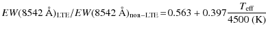
![$\displaystyle \qquad\quad - ~ (0.365 - 0.323\frac{{T}_{\rm eff}}{4500~({\rm K})})[{\rm Fe/H}] - 0.0203[{\rm Fe/H}]^2$](/articles/aa/full_html/2010/05/aa13759-09/img29.png)
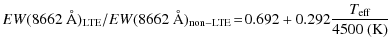
![$\displaystyle \qquad\quad - ~ (0.301 - 0.288\frac{{T}_{\rm eff}}{4500~({\rm K})})[{\rm Fe/H}] - 0.0163[{\rm Fe/H}]^2.$](/articles/aa/full_html/2010/05/aa13759-09/img31.png)
For our finer grid of synthetic spectra from MARCS model atmospheres described in the previous paragraph we use these equations to determine the ratio of LTE to non-LTE equivalent widths for the two lines in each individual model. By dividing the individual equivalent widths in the grid (which are all calculated in LTE) by the factor for the corresponding line before adding the two strongest lines together, we correct each of the grid points for non-LTE effects.
4 The CaT lines at -2.0  [Fe/H]
-0.5
[Fe/H]
-0.5
4.1 The empirical relation
The empirical relation between CaT EW, absolute magnitude
and [Fe/H] is very well studied in globular clusters,
i.e., in the metallicity range between [Fe/H] ![]() -2.3 and [Fe/H]
-2.3 and [Fe/H] ![]() -0.5.
This well-known relation can thus be used to test our synthetic spectra
at these metallicities. We make a comparison between the CaT lines
from atmospheric models between
-0.5 < [Fe/H] < -2.0 and the best fit linear
relation for globular clusters as given in Eqs. (1) and (2) in Sect. 2 (from Battaglia et al. 2008b).
-0.5.
This well-known relation can thus be used to test our synthetic spectra
at these metallicities. We make a comparison between the CaT lines
from atmospheric models between
-0.5 < [Fe/H] < -2.0 and the best fit linear
relation for globular clusters as given in Eqs. (1) and (2) in Sect. 2 (from Battaglia et al. 2008b).
Some approximations are needed to enable a CaT analysis with synthetic spectra which is comparable to observations.
1. The synthetic spectra are all degraded to a resolution of R=6500,
the resolution of VLT/FLAMES used in Medusa mode with the
GIRAFFE LR (LR8) grating as was used in the observational
determination of the empirical relations given above. The equivalent
widths for the two strongest CaT lines are measured using the same
fitting routine as in Battaglia et al. (2008b): a Gaussian fit with a correction which comes from a comparison with a the summed flux contained in a 15 ![]() wide region centered on each line. The correction is necessary to
account for the wings in the strong lines which are distinctly
non-Gaussian in shape. Since the CaT lines can have a variety of
shapes for a range of metallicities, as shown in Fig. 1,
it is in general not advisable to fit them using a single profile.
The disadvantage of using just numerical integration of the observed
spectra is that there are also some weaker lines in this wavelength
range that may vary differently with changing stellar atmospheric
parameters than the CaT lines themselves (Carrera et al. 2007).
Taking these considerations into account, we thus use a combination of
both methods. Weak nearby lines in the spectrum still introduce a small
dependence of the measured CaT EW on resolution though,
since they are more likely to be absorbed into the Gaussian fit at a
lower resolution. This dependence is already present the lowest
metallicity in our grid and gets stronger at higher metallicity,
due to the increasing prominence of the non-Gaussian wings.
wide region centered on each line. The correction is necessary to
account for the wings in the strong lines which are distinctly
non-Gaussian in shape. Since the CaT lines can have a variety of
shapes for a range of metallicities, as shown in Fig. 1,
it is in general not advisable to fit them using a single profile.
The disadvantage of using just numerical integration of the observed
spectra is that there are also some weaker lines in this wavelength
range that may vary differently with changing stellar atmospheric
parameters than the CaT lines themselves (Carrera et al. 2007).
Taking these considerations into account, we thus use a combination of
both methods. Weak nearby lines in the spectrum still introduce a small
dependence of the measured CaT EW on resolution though,
since they are more likely to be absorbed into the Gaussian fit at a
lower resolution. This dependence is already present the lowest
metallicity in our grid and gets stronger at higher metallicity,
due to the increasing prominence of the non-Gaussian wings.
Some of the more prominent weak lines which can be present in the wings of the two strongest CaT lines are the hydrogen Paschen lines. Their strength mainly depends on the temperature of the star (the hotter the stronger) and also to a lesser extend on its gravity (increasing with decreasing gravities). In the more metal-rich part of our grid the Paschen lines fall within the broad wings of the CaT lines and have a direct effect on the EW measurement of the CaT line. However, within the range of parameters we use in our models, the maximum contribution of the Paschen lines to the CaT EW measured is 39 mÅ, which is negligible compared to the total CaT EW. In the more metal-poor part of the grid the CaT lines are narrower and well separated from the Paschen lines. Nonetheless, the Paschen lines can still influence the CaT EW by effecting the placement of the continuum. Also this effect we find to be negligible at our grid parameters, at maximum the CaT EW is changed by 3.5%.
2. Not all the models in our grid, each of them a particular
combination of effective temperature, gravity and metallicity, will
represent real stars on the RGB. To determine which models best
compare to real stars we use two sets of isochrones, the
BaSTI isochrones (Pietrinferni et al. 2004) and the Yonsei-Yale set (e.g., Demarque et al. 2004; Yi et al. 2001).
Both sets can be interpolated to obtain exactly the desired metallicity
and age for a particular isochrone. The Yonsei-Yale set has the
advantage that they go down to [Fe/H] = -3.6 at [![]() /Fe] = +0.4,
whereas the lowest value for the BaSTI set is
[Fe/H] = -2.6. It is well known that different sets of
isochrones do not always give identical results. On top of that,
different ages give (slightly) different parameters for the
RGB stars. In Fig. 3
the grid of models in effective temperature versus gravity is plotted
along with the relations from the theoretical isochrones. In the
two panels the differences due to age, metallicity and the use of
different sets of isochrones are illustrated. Based in Fig. 3 we decide to linearly interpolate in
/Fe] = +0.4,
whereas the lowest value for the BaSTI set is
[Fe/H] = -2.6. It is well known that different sets of
isochrones do not always give identical results. On top of that,
different ages give (slightly) different parameters for the
RGB stars. In Fig. 3
the grid of models in effective temperature versus gravity is plotted
along with the relations from the theoretical isochrones. In the
two panels the differences due to age, metallicity and the use of
different sets of isochrones are illustrated. Based in Fig. 3 we decide to linearly interpolate in ![]() space between the models that are as close as possible to the isochrones and add another 0.25 in
space between the models that are as close as possible to the isochrones and add another 0.25 in ![]() space
on each side to account for uncertainties within the isochrone models
as well as the differences between the isochrones of different ages.
These uncertainties are shown as error bars on the equivalent widths
from synthetic spectra. Note that these represent maximum and minimum
values for the equivalent widths and that these errors
are systematic.
space
on each side to account for uncertainties within the isochrone models
as well as the differences between the isochrones of different ages.
These uncertainties are shown as error bars on the equivalent widths
from synthetic spectra. Note that these represent maximum and minimum
values for the equivalent widths and that these errors
are systematic.
3. Because our synthetic grid is not a stellar system, the
HB magnitude does not have an obvious meaning. Therefore,
to compare our models with empirical relations which require the
height above the HB as an input parameter, we have to rely on
observational or theoretical relations between MV of the HB (
![]() )
of a system and its metallicity. The MV
for each of the grid RGB stars is taken from the isochrones. This
value is consistent with the value we get if we calculate MV from
)
of a system and its metallicity. The MV
for each of the grid RGB stars is taken from the isochrones. This
value is consistent with the value we get if we calculate MV from
![]() using the bolometric correction of giant stars from Alonso et al. (1999). To determine
using the bolometric correction of giant stars from Alonso et al. (1999). To determine
![]() we use the relation given in Catelan & Cortés (2008)
which is calculated using theoretical models for
RR Lyrae stars. Within its uncertainties, this relation is in
excellent agreement with observations of the
we use the relation given in Catelan & Cortés (2008)
which is calculated using theoretical models for
RR Lyrae stars. Within its uncertainties, this relation is in
excellent agreement with observations of the
![]() of globular clusters (e.g., Rich et al. 2005).
of globular clusters (e.g., Rich et al. 2005).
In order to make a fair comparison between the synthetic spectra
and the empirical relation, the atmospheric model properties were
chosen to be as close as possible to known globular cluster properties.
In the atmospheric models we therefore chose to use the alpha-enhanced
models with [![]() /Fe] = +0.4,
except at the higher metallicities ([Fe/H] > -1.0) where
the MARCS grid only provides lower [
/Fe] = +0.4,
except at the higher metallicities ([Fe/H] > -1.0) where
the MARCS grid only provides lower [![]() /Fe] to match observations in the Milky Way. Furthermore, for all [
/Fe] to match observations in the Milky Way. Furthermore, for all [![]() /Fe] = +0.4 models,
[Ca/Fe] was set to +0.25 in the Turbospectrum program, which
even more closely resembles the true values observed in the Galactic
halo globular clusters (e.g., Pritzl et al. 2005). For the isochrone set we use an age of 12 Gyr, comparable to measured ages for the globular clusters (e.g., Krauss & Chaboyer 2003).
We find that for a range of old ages, between 8
and 15 Gyr, the exact choice of the isochrone age does not
significantly affect our results.
/Fe] = +0.4 models,
[Ca/Fe] was set to +0.25 in the Turbospectrum program, which
even more closely resembles the true values observed in the Galactic
halo globular clusters (e.g., Pritzl et al. 2005). For the isochrone set we use an age of 12 Gyr, comparable to measured ages for the globular clusters (e.g., Krauss & Chaboyer 2003).
We find that for a range of old ages, between 8
and 15 Gyr, the exact choice of the isochrone age does not
significantly affect our results.
![\begin{figure}
\par\includegraphics[width=15cm,clip]{13759fg4.eps}
\end{figure}](/articles/aa/full_html/2010/05/aa13759-09/img37.png)
|
Figure 4:
We plot equivalent widths of the two strongest CaT lines which are
measured in the synthetic spectra (symbols) and the empirical relation
from Battaglia et al. (2008b) (black dash-dotted lines) versus (
|
The successful comparison between our synthetic spectra and the
empirical relations, using the BaSTI and the Yonsei-Yale sets of
isochrones, is shown in Fig. 4.
The results for the two different sets of isochrones are comparable,
although the BaSTI isochrones give a slightly better coverage and
agreement at the tip of the RGB. In general, we obtain a good
match between the predictions of our synthetic spectra equivalent
widths and the empirical relation, especially for the most luminous
part of the RGB and at intermediate metallicities where the relation is
best studied. At [Fe/H] = -0.5 the match is clearly
worse, but also the empirical relation is not well constrained at this
metallicity. We also find a larger deviation from the empirical
relation closer to the HB. It was already predicted by Pont et al. (2004) using models that the strength of the CaT lines increases more rapidly for the more luminous part of the RGB. Later, Carrera et al. (2007)
reported a nonlinear tendency in the equivalent width versus absolute
magnitude relation at fainter magnitudes from an observational study of
a large sample of RGB stars in open and globular clusters over a
wide range of magnitudes. Recently, Da Costa et al. (2009)
reported a flattening of the slope of the relation below the HB in
two globular clusters. These observations and early predictions appear
to confirm the effect we see in our synthetic spectra. This trend is
observed to be even stronger below the HB (Da Costa et al. 2009; Carrera et al. 2007), and clearly shows one has to be very cautious applying any of the
![]() relations
to faint stars, especially below the HB. In this paper, we
only focus on the RGB above the HB.
relations
to faint stars, especially below the HB. In this paper, we
only focus on the RGB above the HB.
4.2 Further calibration
In addition to the comparison with the existing empirical relations,
we also calibrate our spectral synthesis models with two (very) well
studied examples, namely the Sun using the Kurucz solar flux atlas (Kurucz et al. 1984) and Arcturus using the Hinkle Arcturus atlas (Hinkle et al. 2000).
Although the match for the Sun is very good, the initial comparison
between the observational Hinkle Arcturus spectrum and the synthesized
spectrum from our models was not satisfactory, especially in the wings
of the strongest CaT line (![]() 8542 Å).
Because this line is extremely broad, it is possible that some of
the outer parts of the line were mistakenly taken to be the continuum
level during the continuum subtraction. After careful renormalization
of the continuum at this wavelength region we were able to get an
acceptable match using the abundances for Arcturus from Fulbright et al. (2007).
8542 Å).
Because this line is extremely broad, it is possible that some of
the outer parts of the line were mistakenly taken to be the continuum
level during the continuum subtraction. After careful renormalization
of the continuum at this wavelength region we were able to get an
acceptable match using the abundances for Arcturus from Fulbright et al. (2007).
5 The CaT lines at [Fe/H] < -2.5
5.1 The empirical relation
Given the success in reproducing the well established calibration of CaT in the range -2.0 ![]() [Fe/H]
[Fe/H] ![]() -0.5, we now extend our synthetic spectral analysis down to [Fe/H] = -4.0. The results are shown in Fig. 5
together with the empirical relation extended linearly to the
low-metallicity regime. We use the Yonsei-Yale isochrone set since it
extends down to the lowest metallicities
-0.5, we now extend our synthetic spectral analysis down to [Fe/H] = -4.0. The results are shown in Fig. 5
together with the empirical relation extended linearly to the
low-metallicity regime. We use the Yonsei-Yale isochrone set since it
extends down to the lowest metallicities![]() . From a comparison of the empirical relation (dash-dotted lines) and the synthetic spectra (colored symbols) in Fig. 5,
it is obvious that the match with the empirical linear relations
breaks down (as expected) at low metallicities, starting from
[Fe/H] < -2.0. For example, the empirical relation
for [Fe/H] = -3.0 lies below the synthetic spectra
predictions for [Fe/H] = -4.0 models for fainter
RGB stars.
. From a comparison of the empirical relation (dash-dotted lines) and the synthetic spectra (colored symbols) in Fig. 5,
it is obvious that the match with the empirical linear relations
breaks down (as expected) at low metallicities, starting from
[Fe/H] < -2.0. For example, the empirical relation
for [Fe/H] = -3.0 lies below the synthetic spectra
predictions for [Fe/H] = -4.0 models for fainter
RGB stars.
![\begin{figure}
\par\includegraphics[width=8.5cm,clip]{13759fg5.eps}
\end{figure}](/articles/aa/full_html/2010/05/aa13759-09/img39.png)
|
Figure 5:
From synthetic analysis we measure the equivalent widths of the two strongest CaT lines as in Fig. 4
extended to lower metallicities. Color coding and symbols for
-2.5 < [Fe/H] < -0.5 is the same as in
Fig. 4,
the additional metallicities are [Fe/H] = -2.5 (purple
squares), [Fe/H] = -3.0 (blue plus signs), and
[Fe/H] = -4.0 (pink crosses). The empirical relations (black
dash-dotted lines), including 1 |
As can be seen in Fig. 5, there is also a trend with the inferred height of a ``star'' above the HB (e.g., surface gravity and temperature) and the deviation of the ``observed'' metallicity compared to the metallicity of the model, for the low-metallicity models. This demonstrates the fact that not just the equivalent width, but also the slope of the relation is changing. At lower metallicities, the equivalent width of the line becomes less sensitive to variations in gravity or temperature of the star (i.e., its position on the RGB).
![\begin{figure}
\par\includegraphics[width=8.5cm,clip]{13759fg6.eps}
\end{figure}](/articles/aa/full_html/2010/05/aa13759-09/img40.png)
|
Figure 6: From synthetic analysis, we plot the ``real'' input value for [Fe/H] in the model versus the ``observed'' value of [Fe/H] for the grid of models, obtained by treating the model spectra as if they were observed in the DART program. For each ``real'' [Fe/H] input value are several points representing RGB stars of the same metallicity at several places along the RGB. Error bars are calculated from the uncertainties shown in Fig. 4 and described in the text. If the CaT method would work perfectly all models should fall (within their uncertainties) on the one-to-one relation shown by the solid black line. Clearly there is an increasing deviation starting at [Fe/H] < -2. Same symbols and color coding used as in Fig. 5. |
The mismatch between the extended empirical relation and the synthetic
modeling predictions at low metallicities is emphasized in Fig. 6
where the input metallicity of the models is plotted versus the
metallicity obtained from the empirical relation as given in Eqs. (1) and (2). From Fig. 6,
we obtain valuable insight into how extremely low-metallicity spectra
would appear in, for instance, the DART sample of
classical dwarf galaxies. While some of the models with input
[Fe/H] ![]() -2.5
are correctly reproduced by the synthetic spectral method, there are
also examples where the metallicity is seriously overestimated. The
linear empirical relation thus offers no means to discriminate between
very low or extremely low metallicity RGB stars.
-2.5
are correctly reproduced by the synthetic spectral method, there are
also examples where the metallicity is seriously overestimated. The
linear empirical relation thus offers no means to discriminate between
very low or extremely low metallicity RGB stars.
6 A new calibration
![\begin{figure}
\par\includegraphics[width=8.5cm,clip]{13759fg7.eps}
\end{figure}](/articles/aa/full_html/2010/05/aa13759-09/img41.png)
|
Figure 7: Same as Fig. 5, but with our new calibration overplotted as thick solid black lines. |
To re-calibrate the relation between the CaT equivalent width and
metallicity for the low-metallicity regime, we use the equivalent
widths obtained from our synthetic spectra. In the relation obtained by
Battaglia et al. (2008b), there are three free parameters to fit the slope of the relation as a function of height above the HB, expressed in W', and a linear relation between W'
and [Fe/H]. To extend this calibration we expect to need at least
two more parameters to fit the dominant features of the low-metallicity
models in one relation: the changing slope with [Fe/H] and the changing
offset between lines of equal metallicity. As input into our
fitting routine we use the results from the synthetic spectra grid from
models described in Table 1 with [![]() /Fe] = +0.4
(and [Ca/Fe] set to +0.25). We use the Yonsei-Yale set of
isochrones, because only those provide the low metallicities needed for
the analysis. For the fitting we use the IDL function MPFIT2DFUN (Markwardt 2009)
to fit a plane relating the absolute magnitude and equivalent widths of
the synthetic models to their metallicity and an F-test to distinguish
the best fit. Not all models are given the same weights in
the fit, for the models both higher up the RGB (
/Fe] = +0.4
(and [Ca/Fe] set to +0.25). We use the Yonsei-Yale set of
isochrones, because only those provide the low metallicities needed for
the analysis. For the fitting we use the IDL function MPFIT2DFUN (Markwardt 2009)
to fit a plane relating the absolute magnitude and equivalent widths of
the synthetic models to their metallicity and an F-test to distinguish
the best fit. Not all models are given the same weights in
the fit, for the models both higher up the RGB (
![]() < -1) and at intermediate metallicities (-1.5
< -1) and at intermediate metallicities (-1.5 ![]() [Fe/H]
[Fe/H] ![]() -0.5)
we give higher weights since these models represent the best studied
region of, and best matching models with, the empirical relation.
Additionally, all models at the (extremely) low-metallicity regime we
are particularly interested in (below [Fe/H] = -2) are
also weighted more. On the other hand, the highest metallicity models
(at [Fe/H] = -0.5) are weighted less, since these have
higher uncertainties and fit less well the empirical relation. Several
functional forms have been explored. The best fit was obtained by a
simple linear relation in both luminosity and equivalent width,
as in the classical empirical calibrations, with merely two extra
terms. One term of equivalent width to the power -1.5 to account
for the variations at low metallicities, one cross term to account for
the slight non-linear slope, as given in Eq. (5).
-0.5)
we give higher weights since these models represent the best studied
region of, and best matching models with, the empirical relation.
Additionally, all models at the (extremely) low-metallicity regime we
are particularly interested in (below [Fe/H] = -2) are
also weighted more. On the other hand, the highest metallicity models
(at [Fe/H] = -0.5) are weighted less, since these have
higher uncertainties and fit less well the empirical relation. Several
functional forms have been explored. The best fit was obtained by a
simple linear relation in both luminosity and equivalent width,
as in the classical empirical calibrations, with merely two extra
terms. One term of equivalent width to the power -1.5 to account
for the variations at low metallicities, one cross term to account for
the slight non-linear slope, as given in Eq. (5).
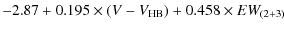
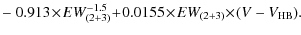
Table 2: The parameters of the observed stars used for verification of the modeling results at low metallicities.
This relation is only calibrated for RGB stars above the HB and
should thus not be applied to stars outside
![]() .
We want to stress that this relation remains ``empirical'', in the
sense that no theoretical arguments are used to find the best fitting
formula. The corresponding fit is shown in Fig. 7,
it fits both the higher metallicity end (and in this regime
the existing empirical relation) and the lower metallicity models well
within their uncertainties. From Fig. 8,
which shows the residual of the fit in the right panel, it can be
seen that the new calibration performs less well at the
high-metallicity end of the calibration ([Fe/H]
.
We want to stress that this relation remains ``empirical'', in the
sense that no theoretical arguments are used to find the best fitting
formula. The corresponding fit is shown in Fig. 7,
it fits both the higher metallicity end (and in this regime
the existing empirical relation) and the lower metallicity models well
within their uncertainties. From Fig. 8,
which shows the residual of the fit in the right panel, it can be
seen that the new calibration performs less well at the
high-metallicity end of the calibration ([Fe/H] ![]() -0.5),
but even there the error is still within a typical observational
error bar for [Fe/H]. We estimate the typical maximum error on the
fitted parameters in Eq. (5) to be
-0.5),
but even there the error is still within a typical observational
error bar for [Fe/H]. We estimate the typical maximum error on the
fitted parameters in Eq. (5) to be ![]() 8%, on the basis of Monte-Carlo simulations of the uncertainties on (
8%, on the basis of Monte-Carlo simulations of the uncertainties on (
![]() )
and the equivalent widths. These reasonably low error values convince
us that the parameters in our new CaT calibration are quite robust
to changes in our approximations.
)
and the equivalent widths. These reasonably low error values convince
us that the parameters in our new CaT calibration are quite robust
to changes in our approximations.
Additionally, in Appendix A, we describe the relation between [Fe/H], EW and MV and MI, to enable the use of the CaT lines as a metallicity estimator for individual RGB stars in systems without a well-defined horizontal branch or for individual RGB field stars.
6.1 Verifying the new calibration at low-metallicity
To verify the reliability of our models at very low-metallicities ([Fe/H] ![]() -2.0),
we have measured the CaT equivalent widths for six low-metallicity
halo stars with existing high-resolution spectroscopic analyses. The
properties of these stars are given in Table 2. Their CaT spectra are degraded to a resolution of R=6500, equal to the resolution of the synthetic spectra grid, and their CaT EWs are measured as described in Sect. 4.1. MV for these halo stars is calculated from
-2.0),
we have measured the CaT equivalent widths for six low-metallicity
halo stars with existing high-resolution spectroscopic analyses. The
properties of these stars are given in Table 2. Their CaT spectra are degraded to a resolution of R=6500, equal to the resolution of the synthetic spectra grid, and their CaT EWs are measured as described in Sect. 4.1. MV for these halo stars is calculated from
![]() using the spectroscopically defined values for gravity and temperature and the bolometric correction of giant stars from Alonso et al. (1999).
Additionally their height above the horizontal branch can be
approximated using their spectroscopic metallicity and the relation
from Catelan & Cortés (2008). In Fig. 9
the results of applying our new CaT calibration to these
observations are shown. There is clearly a very good agreement.
using the spectroscopically defined values for gravity and temperature and the bolometric correction of giant stars from Alonso et al. (1999).
Additionally their height above the horizontal branch can be
approximated using their spectroscopic metallicity and the relation
from Catelan & Cortés (2008). In Fig. 9
the results of applying our new CaT calibration to these
observations are shown. There is clearly a very good agreement.
Additionally, one star from the Boötes I dwarf galaxy as studied by Norris et al. (2010,2008)
using medium- and high-resolution spectroscopy is also plotted.
For this star only one of the two strongest CaT lines could
be measured by Norris et al. (2008) with
confidence, and the total equivalent width for both lines was inferred
using this single line and the observed ratio between the two lines
from Norris et al. (1996,2008)![]() Norris et al. (2008)
find [Fe/H] = -3.45 from medium-resolution spectroscopy using
the Ca II H and K lines, which is very close to the
value we deduce from the EW of the CaT line in the
same spectrum, [Fe/H] = -3.32. In their subsequent
high-resolution follow-up study [Fe/H] is measured directly from
Fe lines, which gives [Fe/H] = -3.7 (Norris et al. 2010).
Norris et al. (2008)
find [Fe/H] = -3.45 from medium-resolution spectroscopy using
the Ca II H and K lines, which is very close to the
value we deduce from the EW of the CaT line in the
same spectrum, [Fe/H] = -3.32. In their subsequent
high-resolution follow-up study [Fe/H] is measured directly from
Fe lines, which gives [Fe/H] = -3.7 (Norris et al. 2010).
![\begin{figure}
\par\includegraphics[width=8.5cm,clip]{13759fg9.eps}\vspace*{-2mm}
\end{figure}](/articles/aa/full_html/2010/05/aa13759-09/img49.png)
|
Figure 9: Plotted with our new CaT calibration (colored lines) are the well-studied RGB stars in the Milky Way halo (black diamonds) and one extremely low-metallicity star in Boötes I (black asterisk) which are all described in Table 2. |
6.2 The DART low-metallicity follow-up program
As a complementary approach to determine if there are any extremely low metallicity stars in the dwarf galaxies, DART has undertaken a follow-up program to obtain HR spectroscopy using the Subaru Telescope High Dispersion Spectrograph, the UVES spectrograph at VLT, and the MIKE spectrograph at Magellan for a sample of stars with CaT [Fe/H] < -2.5 (Aoki et al. 2009; Tafelmeyer et al., in prep.; Venn et al., in prep.). These HR spectra were taken as an addition to the already existing HR spectra from the main program of DART using VLT/FLAMES with the GIRAFFE spectrograph in Medusa mode (Tolstoy et al. 2009; Aoki et al. 2009; Letarte et al., in press; Hill et al., in prep.; Venn et al., in prep.). In these follow-up programmes several extremely low-metallicity stars have been found, with [Fe/H] values below -3.0 (Aoki et al. 2009; Venn et al., in prep.; Tafelmeyer et al., in prep.) and even around -4.0 (Tafelmeyer et al., in prep.). Figure 10 shows all the HR results, compared to their LR [Fe/H] values inferred from the CaT lines using both the old and the new calibration. In this figure the limiting range of the old (linear) calibration is also clearly visible, only the new calibration extends down to the lowest metallicities. For the lower metallicities the error bars become larger, due to the fact that the relations for different metallicities lie closer together and thus a similar error in equivalent width results in a larger error in [Fe/H]. Taking this into account, the new calibration appears to give an accurate prediction of the HR [Fe/H] values.
There are however some stars showing a deviation larger than 1![]() ,
where the most clear example is the extremely metal-poor star in
Fornax. This deviation might be (partly) due to non-LTE effects or
other deficiencies in the modeling of the HR spectrum in order to
derive the stellar parameters and abundances for this really
low-gravity star. Some support of this explanation is the fact that the
agreement between the LR (CaT) and HR results improves when
[Fe II/H] is used instead of [Fe I/H],
most clearly for the extremely metal-poor Fornax star (Tafelmeyer
et al., in prep.). Non-LTE effects are generally
negligible for the dominant ionization state of Fe II (e.g., Thévenin & Idiart 1999; Mashonkina et al. 2010; Kraft & Ivans 2003), however for Fe I the non-LTE effects are expected to be more significant in low-metallicity, low-gravity stars (e.g., Thévenin & Idiart 1999; Mashonkina et al. 2010; Gehren et al. 2001).
,
where the most clear example is the extremely metal-poor star in
Fornax. This deviation might be (partly) due to non-LTE effects or
other deficiencies in the modeling of the HR spectrum in order to
derive the stellar parameters and abundances for this really
low-gravity star. Some support of this explanation is the fact that the
agreement between the LR (CaT) and HR results improves when
[Fe II/H] is used instead of [Fe I/H],
most clearly for the extremely metal-poor Fornax star (Tafelmeyer
et al., in prep.). Non-LTE effects are generally
negligible for the dominant ionization state of Fe II (e.g., Thévenin & Idiart 1999; Mashonkina et al. 2010; Kraft & Ivans 2003), however for Fe I the non-LTE effects are expected to be more significant in low-metallicity, low-gravity stars (e.g., Thévenin & Idiart 1999; Mashonkina et al. 2010; Gehren et al. 2001).
7 Alpha element dependence on the CaT lines
It is naturally expected that differences in [Ca/Fe] will significantly
change the equivalent width of the CaT lines, and therefore alter
the observed relation between equivalent width and [Fe/H]. The
MARCS collaboration also provides model atmospheres where the ![]() elements are not enhanced, but are kept similar to the ratio in the Sun for all models with [Fe/H]
elements are not enhanced, but are kept similar to the ratio in the Sun for all models with [Fe/H] ![]() -2. Figure 11
shows that we recover this difference in our synthetic spectra.
Qualitatively, the space between the enhanced and solar
[Ca/Fe] models at equal [Fe/H] seems to agree with the step
taken in abundance. The equivalent width in our grid of synthetic
spectra does trace the Ca abundance. Since the strength of any
line depends on the line opacity divided by the continuous opacity,
it is expected that also other elements than Ca can affect the
CaT line EW. If these elements contribute free electrons these can enhance the H- concentration
and therefore affect the continuous opacity. Which element contributes
most free electrons is dependent on the effective temperature and layer
of the atmosphere of the star in consideration, but for cool
stellar atmospheres in general the main sources of electrons are Mg,
Fe, Si, Ca, Na, and Al (Shetrone et al. 2009). Since thus both Fe and some of the
-2. Figure 11
shows that we recover this difference in our synthetic spectra.
Qualitatively, the space between the enhanced and solar
[Ca/Fe] models at equal [Fe/H] seems to agree with the step
taken in abundance. The equivalent width in our grid of synthetic
spectra does trace the Ca abundance. Since the strength of any
line depends on the line opacity divided by the continuous opacity,
it is expected that also other elements than Ca can affect the
CaT line EW. If these elements contribute free electrons these can enhance the H- concentration
and therefore affect the continuous opacity. Which element contributes
most free electrons is dependent on the effective temperature and layer
of the atmosphere of the star in consideration, but for cool
stellar atmospheres in general the main sources of electrons are Mg,
Fe, Si, Ca, Na, and Al (Shetrone et al. 2009). Since thus both Fe and some of the ![]() elements have to be considered as important electron donors, this can significantly affect the dependence of the CaT EW on the [
elements have to be considered as important electron donors, this can significantly affect the dependence of the CaT EW on the [![]() /Fe] ratio.
Nevertheles we find that, within the abundance parameters we adopt in
this study, the Ca abundance itself is by far the dominant
factor determining the EW of the CaT line, as can be seen in Fig. 11.
/Fe] ratio.
Nevertheles we find that, within the abundance parameters we adopt in
this study, the Ca abundance itself is by far the dominant
factor determining the EW of the CaT line, as can be seen in Fig. 11.
However, when comparing the sensitivity of the CaT equivalent width
measurements of RGB stars in Sculptor and Fornax with
high-resolution [Fe/H] and [Ca/H] measurements Battaglia et al. (2008b)
find that the CaT equivalent width is actually a more robust estimator
of Fe than Ca. This would suggest that it is therefore not
advisable to use the CaT as a linear estimator for [Ca/H] (see Battaglia et al. 2008b, and their Figs. 10 and 12). This result is not expected from the theoretical expectations shown in Fig. 11.
There are several factors that may contribute to this apparent
discrepancy between the modeling and observational results. First,
in our grid of synthetic spectra we assume the relative abundance
of Ca to the other ![]() elements
to stay constant, an assumption that not necessarily holds for all
RGB stars. The extra free electrons donated by the other
elements
to stay constant, an assumption that not necessarily holds for all
RGB stars. The extra free electrons donated by the other ![]() elements might affect the strength of the CaT line through the continuous opacity as described above. Shetrone et al. (2009)
find that a 0.5 dex decrease in the electron contributors can
increase the CaT line strength enough to mimic
a Ca abundance increase of
elements might affect the strength of the CaT line through the continuous opacity as described above. Shetrone et al. (2009)
find that a 0.5 dex decrease in the electron contributors can
increase the CaT line strength enough to mimic
a Ca abundance increase of ![]() 0.2 or even
0.2 or even ![]() 0.4
depending on the atmosphere parameters of the star. However,
in Fornax we generally find that the important electron donors Fe
and Mg are increased relatively to the values in our grid at
similar [Ca/H], while we still measure the CaT lines to be
too strong relative to the [Ca/H] measurements directly from Ca I lines.
This result clearly indicates that the effect of electron donors can
not be driving the offset between [Ca/H] derived from CaT and
HR Ca I analyses. Second, the HR Ca abundances are usually derived from fewer Ca I lines compared to the large number of HR Fe I lines available and are therefore subject to larger observational errors. Third, the HR determination of the Ca I abundance is subject to non-LTE effects (Mashonkina et al. 2007).
If non-LTE effects are included in the analysis of the
HR spectra to determine the Ca abundances this might lead to
a closer match in Ca abundances derived from the Ca I and CaT lines. To investigate this more closely we have modeled both the Ca I
and CaT line strengths using abundances and atmospheric parameters
from the well-studied halo star CD -38 245 (e.g., Cayrel et al. 2004) as a test case. The modeling, using the same models and techniques as described in Sect. 3.2,
is performed for [Ca/Fe] = +0.4 in LTE and non-LTE to
determine the offset from non-LTE to LTE abundances. The results
are shown in Table 3. It can be seen that the LTE approximation has an effect on the determination of the Ca abundance from the Ca I lines (a difference of over 0.2 dex for the Ca I line at
0.4
depending on the atmosphere parameters of the star. However,
in Fornax we generally find that the important electron donors Fe
and Mg are increased relatively to the values in our grid at
similar [Ca/H], while we still measure the CaT lines to be
too strong relative to the [Ca/H] measurements directly from Ca I lines.
This result clearly indicates that the effect of electron donors can
not be driving the offset between [Ca/H] derived from CaT and
HR Ca I analyses. Second, the HR Ca abundances are usually derived from fewer Ca I lines compared to the large number of HR Fe I lines available and are therefore subject to larger observational errors. Third, the HR determination of the Ca I abundance is subject to non-LTE effects (Mashonkina et al. 2007).
If non-LTE effects are included in the analysis of the
HR spectra to determine the Ca abundances this might lead to
a closer match in Ca abundances derived from the Ca I and CaT lines. To investigate this more closely we have modeled both the Ca I
and CaT line strengths using abundances and atmospheric parameters
from the well-studied halo star CD -38 245 (e.g., Cayrel et al. 2004) as a test case. The modeling, using the same models and techniques as described in Sect. 3.2,
is performed for [Ca/Fe] = +0.4 in LTE and non-LTE to
determine the offset from non-LTE to LTE abundances. The results
are shown in Table 3. It can be seen that the LTE approximation has an effect on the determination of the Ca abundance from the Ca I lines (a difference of over 0.2 dex for the Ca I line at ![]() = 6162
= 6162 ![]() ). In the LTE approximation, the agreement between the abundances derived from the Ca I and CaT lines is very poor, CaT analysis results in a Ca abundance much greater than for Ca I.
In non-LTE, we are able to reproduce better all the measured
Ca features in an extremely metal-poor star. The remaining
discrepancy probably relates to the outer atmospheric layers that are
not very well modeled - even in non-LTE. To fully resolve the
discrepancy between the Ca I and CaT results,
one would have to properly explore the effects of specific details
including line profile fitting and uncertainties in the stellar
parameters.
). In the LTE approximation, the agreement between the abundances derived from the Ca I and CaT lines is very poor, CaT analysis results in a Ca abundance much greater than for Ca I.
In non-LTE, we are able to reproduce better all the measured
Ca features in an extremely metal-poor star. The remaining
discrepancy probably relates to the outer atmospheric layers that are
not very well modeled - even in non-LTE. To fully resolve the
discrepancy between the Ca I and CaT results,
one would have to properly explore the effects of specific details
including line profile fitting and uncertainties in the stellar
parameters.
The stars in the dataset described by Battaglia et al. (2008b) which show the largest discrepancies in CaT compared to [Ca/H], are typically much more metal-rich RGB stars than CD -38 245. For this regime we have not modeled the non-LTE effects in Ca I lines. Most of the discrepant stars are from the Fornax dwarf galaxy, where we were just able to target its brightest population of RGB stars due to the relatively large distance to this dwarf galaxy (see also Sect. 8.2). This means we are also statistically probing closer to the tip of the RGB, where we find the lower gravity stars for which the outer layers are more diffuse and thus more difficult to model - certainly assuming LTE.
Table 3: Ca abundances for CD -38 245.
8 Implications for the DART survey
Our new CaT-[Fe/H] calibration enables a more direct search for
extremely metal-poor stars in existing datasets, like the large
DART sample of CaT measurements in RGB stars of four
classical dwarf galaxies (Sculptor, Fornax, Carina, and Sextans). These
DART samples were observed in LR (![]() )
Medusa mode using the European Southern Observatory (ESO) VLT/FLAMES facility (Pasquini et al. 2002) and are described in Helmi et al. (2006), Koch et al. (2006) and Battaglia et al. (2008a,b,2006).
)
Medusa mode using the European Southern Observatory (ESO) VLT/FLAMES facility (Pasquini et al. 2002) and are described in Helmi et al. (2006), Koch et al. (2006) and Battaglia et al. (2008a,b,2006).
In Fig. 12 we
overplot the complete low-resolution samples for the four galaxies
observed in the DART program, Sculptor, Fornax, Carina and
Sextans, along with the new CaT calibration (colored lines). All
observed RGB stars, which are likely to be members, from DART are
shown as small gray circles. All stars have a signal-to-noise ratio
larger than 10 (per Å), a velocity error smaller
than 5 km s-1 and a velocity which is within 3![]() of the systemic radial velocity of the galaxy (for Fornax 2.5
of the systemic radial velocity of the galaxy (for Fornax 2.5![]() is used, because of the larger contribution from Milky Way foreground). These criteria are identical to those applied by Battaglia et al. (2008a,2006). We use
is used, because of the larger contribution from Milky Way foreground). These criteria are identical to those applied by Battaglia et al. (2008a,2006). We use
![]() for the dwarf galaxies as given in Irwin & Hatzidimitriou (1995). For the errors in the sum of equivalent widths we use the results of Battaglia et al. (2008b)
who found that the random error from repeated measurements of the
low-resolution sample in the sum of the two broadest lines is well
represented by
for the dwarf galaxies as given in Irwin & Hatzidimitriou (1995). For the errors in the sum of equivalent widths we use the results of Battaglia et al. (2008b)
who found that the random error from repeated measurements of the
low-resolution sample in the sum of the two broadest lines is well
represented by
![]()
![]() 6/(S/N). Although this error can be quite extensive (mean error bars per galaxy and luminosity bin are shown in Fig. 12),
there are clearly a number of stars in these galaxies that are
predicted to have [Fe/H] < -3. Our low-metallicity
candidates need to be followed up with high-resolution spectroscopy to
verify our prediction. A small sample of low-metallicity
candidates has already been followed up with high-resolution
spectroscopy within DART, these results are discussed in Sect. 6.2 and in Aoki et al. (2009),
Tafelmeyer et al. (in prep.) and Venn et al.
(in prep.). The extremely metal-poor stars discovered within these
DART follow-up programs in Sculptor, Fornax, Carina, and Sextans and
the one extremely metal-poor Sculptor star discovered by Kirby et al. (2009) and Frebel et al. (2010)
already provide an independent confirmation of our predictions of the
existence of extremely low-metallicity stars in these classical
dwarf galaxies.
6/(S/N). Although this error can be quite extensive (mean error bars per galaxy and luminosity bin are shown in Fig. 12),
there are clearly a number of stars in these galaxies that are
predicted to have [Fe/H] < -3. Our low-metallicity
candidates need to be followed up with high-resolution spectroscopy to
verify our prediction. A small sample of low-metallicity
candidates has already been followed up with high-resolution
spectroscopy within DART, these results are discussed in Sect. 6.2 and in Aoki et al. (2009),
Tafelmeyer et al. (in prep.) and Venn et al.
(in prep.). The extremely metal-poor stars discovered within these
DART follow-up programs in Sculptor, Fornax, Carina, and Sextans and
the one extremely metal-poor Sculptor star discovered by Kirby et al. (2009) and Frebel et al. (2010)
already provide an independent confirmation of our predictions of the
existence of extremely low-metallicity stars in these classical
dwarf galaxies.
8.1 Old and new calibration: a comparison
It should be noted that the total number of stars affected by the
new calibration in the DART CaT surveys is very small. In the
current DART data set, just 2.5% of the target stars have a
metallicity below [Fe/H] = -2.5, using the calibration of Battaglia et al. (2008b).
Using the new calibration the fraction of low-metallicity stars
increases somewhat to about 7.5%. Still it is important to realize
that ![]() 92.5% of the stars in these systems are at a metallicity which is consistent with both the calibration of Battaglia et al. (2008b) and that given in Sect. 6
of this paper. This implies that the number of low-metallicity
candidates remains very small compared to the total number of observed
stars. This result is illustrated in Fig. 13
where we compare the metallicity distributions for each galaxy using
two calibrations of the CaT data: the calibration for dwarf
galaxies published by Battaglia et al. (2008b)
(in black), and the re-calibration presented here (in red).
It is clear that the overall distributions of metallicities within
these galaxies do not change significantly for the different
CaT calibrations, the only clear differences are in the
low-metallicity tails which have become more populated and more
extended with the new CaT calibration.
92.5% of the stars in these systems are at a metallicity which is consistent with both the calibration of Battaglia et al. (2008b) and that given in Sect. 6
of this paper. This implies that the number of low-metallicity
candidates remains very small compared to the total number of observed
stars. This result is illustrated in Fig. 13
where we compare the metallicity distributions for each galaxy using
two calibrations of the CaT data: the calibration for dwarf
galaxies published by Battaglia et al. (2008b)
(in black), and the re-calibration presented here (in red).
It is clear that the overall distributions of metallicities within
these galaxies do not change significantly for the different
CaT calibrations, the only clear differences are in the
low-metallicity tails which have become more populated and more
extended with the new CaT calibration.
![\begin{figure}
\par\includegraphics[width=8.5cm,clip]{13759fg13.eps}
\end{figure}](/articles/aa/full_html/2010/05/aa13759-09/img55.png)
|
Figure 13: Distributions of [Fe/H] for the four dwarf spheroidal galaxies in the DART survey, using both the old calibration (Eqs. (1) and (2), black) and the new calibration (Eq. (5), red) of the CaT lines. The error bars are Poissonian. |
8.2 The low-metallicity tails
![\begin{figure}
\par\includegraphics[width=8.5cm,clip]{13759fg14.eps}
\end{figure}](/articles/aa/full_html/2010/05/aa13759-09/img56.png)
|
Figure 14: The low-metallicity tails of the four classical dwarf galaxies studied by DART as obtained with the new calibration presented here. In the top panel these are normalized at [Fe/H] = -2.5 and compared to the low-metallicity tails from the HES survey (both corrected and raw) from Schörck et al. (2009) and a compilation of ultra-faint dwarf galaxies (Kirby et al. 2008). The bottom panel displays the same low-metallicity tails for the classical- and ultra-faint dwarf galaxies, but normalized to the total number of observed stars in each system. |
Although their number is small relative to the total number of observed
stars, the (extremely) metal-poor stars in each of these galaxies
represents an important and interesting component of the overall
stellar population. The low-metallicity population can reveal details
of the chemical evolution of a particular galaxy and, by comparison,
of the differences and similarities of the early evolutionary
stages of galaxies. In Fig. 14
we show a comparison of the low-metallicity tails from individual
stars, without application of binning or error estimates, in the
four classical dwarf galaxies of DART using our new calibration for the
CaT equivalent widths and in an ensemble of ultra-faint dwarf galaxies
using low-resolution (R ![]() 6500) spectra over a large wavelength range compared with an extensive spectral library (Kirby et al. 2008) and the HES survey of the Milky Way halo (Schörck et al. 2009) measuring [Fe/H] from a combination of indices for the Ca II K and H
6500) spectra over a large wavelength range compared with an extensive spectral library (Kirby et al. 2008) and the HES survey of the Milky Way halo (Schörck et al. 2009) measuring [Fe/H] from a combination of indices for the Ca II K and H![]() lines.
Since the number of stars present, and observed, in these systems
can vary quite a lot, a crucial step in comparing the
low-metallicity tails is to normalize them at a certain metallicity or
to a certain total number of measurements. In the upper panel of
Fig. 14 all the
low-metallicity tails have been normalized to 1 at
[Fe/H] = -2.5. In this way, one can compare the shape of
the metallicity tails below this value of [Fe/H] assuming all
surveys are equally complete at this level. In the lower panel we have
normalized to the total number of stars observed in each system
to give a feeling for the relative number of (extremely)
low-metallicity stars observed. Ideally, one would like to be able to
isolate the first generation of stars in all these galaxies and compare
these populations. With our current understanding it is not possible to
make such a clear distinction between samples, which is why we resort
to the methods shown in Fig. 14.
However, with future larger samples of stars with accurate abundances
in these galaxies one could envision making use of the position of the
knee in the [
lines.
Since the number of stars present, and observed, in these systems
can vary quite a lot, a crucial step in comparing the
low-metallicity tails is to normalize them at a certain metallicity or
to a certain total number of measurements. In the upper panel of
Fig. 14 all the
low-metallicity tails have been normalized to 1 at
[Fe/H] = -2.5. In this way, one can compare the shape of
the metallicity tails below this value of [Fe/H] assuming all
surveys are equally complete at this level. In the lower panel we have
normalized to the total number of stars observed in each system
to give a feeling for the relative number of (extremely)
low-metallicity stars observed. Ideally, one would like to be able to
isolate the first generation of stars in all these galaxies and compare
these populations. With our current understanding it is not possible to
make such a clear distinction between samples, which is why we resort
to the methods shown in Fig. 14.
However, with future larger samples of stars with accurate abundances
in these galaxies one could envision making use of the position of the
knee in the [![]() /Fe] ratios for example (Tolstoy et al. 2009) to select the first generations of stars in each galaxy.
/Fe] ratios for example (Tolstoy et al. 2009) to select the first generations of stars in each galaxy.
Before interpreting these metallicity tails further we stress that there are several caveats which prevent us from a detailed analysis of these results at face value.
First, the errors on the individual measurements are large, especially
at low [Fe/H] and/or for fainter stars (typical error bars are
shown in Fig. 12)
and asymmetric. The asymmetry and dependence on metallicity arise from
the fact that the relation between [Fe/H] and equivalent width is
not linear at low metallicities, since the lines of equal metallicity
are closer together. A symmetric error bar in the measured
equivalent width, therefore results in a much larger error downwards
than upwards in [Fe/H]. For instance, the one star in
the Sextans dwarf galaxy that falls below the
[Fe/H] = -4 calibration (see Fig. 12) will be assigned a very low metallicity using the calibration, which causes the Sextans curve in Fig. 14 to stay above zero at [Fe/H] = -4.5. However, the upper 1![]() error in equivalent width allows a metallicity of [Fe/H] = -3.8.
error in equivalent width allows a metallicity of [Fe/H] = -3.8.
Second, there are several selection and/or sampling effects that are difficult to correct for. For example, the fact that not all stars have been observed in all of these systems. For instance, a much larger percentage of the Sextans stars have been observed than Fornax stars, although the total sample in Fornax is larger (it is a larger galaxy). Also, the absolute magnitude range of the populations targeted may not be comparable. From Fig. 12 it can clearly be seen that in Fornax, for instance, only stars well within 2 mag from the tip of the RGB are observed due to its larger distance, while in the other galaxies the samples extend to fainter stars. Any luminosity bias that might remain in our new calibration would therefore result in a different bias for different galaxies in the extent and population of the low-metallicity tails. Even if one would observe the same range of magnitudes from the tip of the RGB for all galaxies, this could still introduce a bias, because of age and metallicity effects on the RGB for an extended star formation history. Additionally, some galaxies possess metallicity gradients (e.g., Tolstoy et al. 2004; Battaglia et al. 2006), which means that the final metallicity distribution can also be greatly affected by the spatial sampling within a galaxy.
Thus, even though from Fig. 14 one might be tempted to conclude that the low-metallicity tail of Fornax is different in both shape and number from the other classical dwarf galaxies and the halo and it must therefore have had a different chemical history in the earliest epochs, it is not at all clear whether such a conclusion is justified. It is very well possible that the low-metallicity tail of Fornax lies hidden under its very dominant, relatively young, metal-rich population and we have not been able to retrieve it because we sample a very small fraction of the total number of RGB stars in this galaxy.
However, from the top panel of Fig. 14 it is clear that the significant difference between the metal-poor tail in the halo and in the dwarf galaxies from Helmi et al. (2006) has disappeared. This also brings the metallicity distribution function for the classical dSphs in line with the results of Kirby et al. (2008) for the ultra-faint dwarf galaxies. The shapes of the low-metallicity tails, normalized at [Fe/H] = -2.5, are now much more similar.
9 Conclusions
It is important for our understanding of galactic chemical evolution
to know whether there are just a few, and in this case how many,
extremely low-metallicity ([Fe/H] ![]() -3)
stars in the classical dSph galaxies, or none at all. This
can change our view of their early evolution and their subsequent role
in galaxy formation and evolution. Subsequently, this will influence
our view on the present-day satellite galaxies as possible templates
for the building blocks which formed the Galactic halo and their
relation to the more metal-poor ultra-faint dwarf galaxies.
-3)
stars in the classical dSph galaxies, or none at all. This
can change our view of their early evolution and their subsequent role
in galaxy formation and evolution. Subsequently, this will influence
our view on the present-day satellite galaxies as possible templates
for the building blocks which formed the Galactic halo and their
relation to the more metal-poor ultra-faint dwarf galaxies.
Using a grid of synthetic spectra based on MARCS atmosphere
models we have investigated the behavior of the three
CaT absorption lines as metallicity indicators over a range of
metallicities from [Fe/H] = -0.5 down to
[Fe/H] = -4. Our models agree with the well-known observed
linear relations at [Fe/H] ![]() -2.0, although small deviations from linearity are found closer to the HB as were already predicted and observed (Pont et al. 2004; Carrera et al. 2007).
For [Fe/H] < -2.0, the relations of equal metallicity
get closer together and are flatter as a function of absolute
magnitude. This behavior was expected and is reflected in the change in
the profile of the CaT lines, from wing-dominated to
core-dominated as the metallicity drops. We have provided a new
calibration taking this behavior into account, which we have
successfully tested on several well-known low-metallicity giant stars.
We have also investigated the role of the Ca abundance itself on
these lines and found that although the lines ought to trace Ca
instead of Fe, this often is not observed, probably due to
inaccuracies in the determination of the HR Ca abundance.
-2.0, although small deviations from linearity are found closer to the HB as were already predicted and observed (Pont et al. 2004; Carrera et al. 2007).
For [Fe/H] < -2.0, the relations of equal metallicity
get closer together and are flatter as a function of absolute
magnitude. This behavior was expected and is reflected in the change in
the profile of the CaT lines, from wing-dominated to
core-dominated as the metallicity drops. We have provided a new
calibration taking this behavior into account, which we have
successfully tested on several well-known low-metallicity giant stars.
We have also investigated the role of the Ca abundance itself on
these lines and found that although the lines ought to trace Ca
instead of Fe, this often is not observed, probably due to
inaccuracies in the determination of the HR Ca abundance.
The new calibration of the
![]() relation described here therefore provides a reliable updated method to
search for low-metallicity stars using just the equivalent widths of
two CaT lines. This method requires only a small wavelength range
of the spectrum at low resolution and the absolute magnitude of
the star.
relation described here therefore provides a reliable updated method to
search for low-metallicity stars using just the equivalent widths of
two CaT lines. This method requires only a small wavelength range
of the spectrum at low resolution and the absolute magnitude of
the star.
Applying the new calibration to the DART data sets shows that, although low in relative number, there are several extremely low-metallicity RGB candidates in these classical dwarf galaxies that deserve further study. This new calibration thus opens possibilities to study the (extremely) metal-poor tail that makes up only a small, but interesting, fraction of the dwarf galaxy stellar populations.
AcknowledgementsWe would like to warmly thank Jon Fulbright and Wako Aoki for sharing their CaT spectra of halo RGB stars with us and Bertrand Plez for making his linelists and Turbospectrum code available. We also thank Evan Kirby for supplying his data for the low-metallicity tail for the ultra-faint dwarfs and the referee, George Wallerstein, for useful suggestions that helped improve the paper. E.S., E.T., A.H., and T.d.B. gratefully acknowledge Netherlands Foundation for Scientific Research (NWO) and the Netherlands Research School for Astronomy (NOVA) for financial support. V.H. acknowledges the financial support of the Programme National Galaxies (PNG) of the Institut National des Sciences de l'Univers (INSU). A.H. was supported by the ERC-StG Galactica 240271. J.I.G.H. acknowledges financial support from EU contract MEXT-CT-2004-014265 (CIFIST) and from the Spanish Ministry project MICINN AYA2008-00695. This work has made use of BaSTI web tools.
Appendix A: Absolute magnitude [Fe/H] and [Ca/H] calibrations
In numerous studies the equivalent widths of the CaT lines are
studied in relation to the height of the stars above the HB. While
this measure is very convenient for the study of stars in (galactic)
globular clusters, one might also want to study systems which have no
well-defined HB magnitude, or even no HB at all. In
the main body of the paper we have chosen to define an extended
calibration of the CaT equivalent width as a function of
![]() ), which also enabled a direct comparison with the empirical relation of Battaglia et al. (2008b). Here we also provide a calibration directly to (Johnson-Cousins) MV and MI.
Note that this also means that we can remove the assumption regarding
the HB magnitude of our modeled ``RGB stars''. An extra
advantage of using MI (instead of MV)
is that it is much less sensitive to age effects, and therefore
provides more accurate metallicities for, in particular, younger
populations of stars (Carrera et al. 2007). We also provide calibrations for [Ca/H] instead of [Fe/H], using our full modeling grid of Table 1 including the models with solar [
), which also enabled a direct comparison with the empirical relation of Battaglia et al. (2008b). Here we also provide a calibration directly to (Johnson-Cousins) MV and MI.
Note that this also means that we can remove the assumption regarding
the HB magnitude of our modeled ``RGB stars''. An extra
advantage of using MI (instead of MV)
is that it is much less sensitive to age effects, and therefore
provides more accurate metallicities for, in particular, younger
populations of stars (Carrera et al. 2007). We also provide calibrations for [Ca/H] instead of [Fe/H], using our full modeling grid of Table 1 including the models with solar [![]() /Fe] values. All calibrations use the same functional form given in Eq. (A.1). The parameters for both [Fe/H] and [Ca/H] using either
/Fe] values. All calibrations use the same functional form given in Eq. (A.1). The parameters for both [Fe/H] and [Ca/H] using either
![]() ), MV, or MI are given in Table A.1.
), MV, or MI are given in Table A.1.
![$\displaystyle \textnormal[{\rm Fe}/{\rm H}]{\rm\ or \ [{\rm Ca}/{\rm H}]} = a + b \times{\rm (Abs.\ mag.)} + c \times EW_{(2+3)}$](/articles/aa/full_html/2010/05/aa13759-09/img59.png)

Table A.1: Best fitting parameters for the new calibrations.
![\begin{figure}
\par\includegraphics[width=8.5cm,clip]{13759fg15.eps}\vspace*{2mm}
\includegraphics[width=8.5cm,clip]{13759fg16.eps}
\end{figure}](/articles/aa/full_html/2010/05/aa13759-09/img61.png)
|
Figure A.1: Top panels: same as Fig. 10, but now on the y-axis the new calibration for MV and MI are plotted. Bottom panels: the new calibration for [Ca/H] using either MV or MI. |
Since also these relations are only calibrated for RGB stars and
above the HB, they should thus not be applied to stars outside
![]() ,
-3 < MV < 0.8, or
-4 < MI < 0.
In Fig. A.1, we show the results of the calibrations using MV and MI
for the high-resolution DART sample for both [Fe/H]
and [Ca/H]. Distance moduli for Sculptor, Fornax, Carina and
Sextans are taken from Kaluzny et al. (1995), Rizzi et al. (2007), Mateo et al. (1998), and Mateo et al. (1995)
respectively. The results do not change significantly depending on
which absolute magnitude is used, as can also be seen from a
comparison of the upper panels of Figs. A.1 with 10. It remains clear from Fig. A.1,
that our new CaT calibrations based on the synthesized spectra
trace the HR [Fe/H] values much better than HR [Ca/H],
as was already discussed in Sect. 7 of this paper and found by Battaglia et al. (2008b).
,
-3 < MV < 0.8, or
-4 < MI < 0.
In Fig. A.1, we show the results of the calibrations using MV and MI
for the high-resolution DART sample for both [Fe/H]
and [Ca/H]. Distance moduli for Sculptor, Fornax, Carina and
Sextans are taken from Kaluzny et al. (1995), Rizzi et al. (2007), Mateo et al. (1998), and Mateo et al. (1995)
respectively. The results do not change significantly depending on
which absolute magnitude is used, as can also be seen from a
comparison of the upper panels of Figs. A.1 with 10. It remains clear from Fig. A.1,
that our new CaT calibrations based on the synthesized spectra
trace the HR [Fe/H] values much better than HR [Ca/H],
as was already discussed in Sect. 7 of this paper and found by Battaglia et al. (2008b).
Appendix B: Ratio of the 8542 Å to the 8662 Å CaT line
![\begin{figure}
\par\includegraphics[width=8.5cm,clip]{13759fg17.eps}
\end{figure}](/articles/aa/full_html/2010/05/aa13759-09/img62.png)
|
Figure B.1:
The ratio of the second (8542 |
Another useful application of our models is the investigation of the
ratios between the line strengths of the CaT lines, as a
function of [Fe/H] and luminosity. This enables the determination
of the summed equivalent width if just one of the two strongest lines
are present or usable in the spectrum of a star. Additionally,
investigation of the relative differences in development of the lines
for various combinations of atmospheric parameters can give valuable
insights into the line formation process. In Fig. B.1 the ratios between the EWs of the second and third CaT lines, both of which are first corrected for non-LTE effects using Eqs. (3) and (4),
are plotted as a function of [Fe/H] for a synthetic ``giant''
spectrum. The variation in the ratio with absolute magnitude turns out
to be very small as can be seen from the dispersion of the equal
metallicity models. Although for the intermediate metallicity
(-3 < [Fe/H] < -1) spectra the ratio seems
roughly constant with metallicity, the ratio changes significantly at
higher ([Fe/H] = -0.5), or extremely low
([Fe/H] = -4) metallicities. We also find that the value for
intermediate metallicities is somewhat lower than the value
of 1.34 as measured by Norris et al. (2008). Our mean ratio from the models is 1.27 if all models -2.5 ![]() [Fe/H]
[Fe/H] ![]() -0.5
are taken into account (this particular range is chosen since it
represents the metallicities of the vast majority of stars in the
classical dwarf spheroidal galaxies). This value is confirmed in a
comparison with the observed spectra from the DART dataset where a
very similar mean value is found although the spread is much larger due
to the observational uncertainties.
-0.5
are taken into account (this particular range is chosen since it
represents the metallicities of the vast majority of stars in the
classical dwarf spheroidal galaxies). This value is confirmed in a
comparison with the observed spectra from the DART dataset where a
very similar mean value is found although the spread is much larger due
to the observational uncertainties.
References
- Alonso, A., Arribas, S., & Martínez-Roger, C. 1999, A&AS, 140, 261 [NASA ADS] [CrossRef] [EDP Sciences] [Google Scholar]
- Alvarez, R., & Plez, B. 1998, A&A, 330, 1109 [NASA ADS] [Google Scholar]
- Aoki, W., Arimoto, N., Sadakane, K., et al. 2009, A&A, 502, 569 [NASA ADS] [CrossRef] [EDP Sciences] [Google Scholar]
- Armandroff, T. E., & Zinn, R. 1988, AJ, 96, 92 [NASA ADS] [CrossRef] [Google Scholar]
- Armandroff, T. E., & Da Costa, G. S. 1991, AJ, 101, 1329 [NASA ADS] [CrossRef] [Google Scholar]
- Barklem, P. S., Christlieb, N., Beers, T. C., et al. 2005, A&A, 439, 129 [NASA ADS] [CrossRef] [EDP Sciences] [Google Scholar]
- Battaglia, G., Tolstoy, E., Helmi, A., et al. 2006, A&A, 459, 423 [NASA ADS] [CrossRef] [EDP Sciences] [Google Scholar]
- Battaglia, G., Helmi, A., Tolstoy, E., et al. 2008a, ApJ, 681, L13 [Google Scholar]
- Battaglia, G., Irwin, M., Tolstoy, E., et al. 2008b, MNRAS, 383, 183 [Google Scholar]
- Butler, K., & Giddings, J. R. 1985, Newsletter of Analysis of Astronomical Spectra, 9 [Google Scholar]
- Carrera, R., Gallart, C., Pancino, E., & Zinn, R. 2007, AJ, 134, 1298 [NASA ADS] [CrossRef] [Google Scholar]
- Castelli, F., & Kurucz, R. L. 2003, in Modelling of Stellar Atmospheres, ed. N. Piskunov, W. W. Weiss, & D. F. Gray, IAU Symp., 210, 20P [Google Scholar]
- Catelan, M., & Cortés, C. 2008, ApJ, 676, L135 [NASA ADS] [CrossRef] [Google Scholar]
- Cayrel, R., Depagne, E., Spite, M., et al. 2004, A&A, 416, 1117 [NASA ADS] [CrossRef] [EDP Sciences] [Google Scholar]
- Cenarro, A. J., Cardiel, N., Gorgas, J., et al. 2001, MNRAS, 326, 959 [NASA ADS] [CrossRef] [Google Scholar]
- Cenarro, A. J., Gorgas, J., Cardiel, N., Vazdekis, A., & Peletier, R. F. 2002, MNRAS, 329, 863 [NASA ADS] [CrossRef] [Google Scholar]
- Cohen, J. G. 1978, ApJ, 221, 788 [NASA ADS] [CrossRef] [Google Scholar]
- Cohen, J. G., & Huang, W. 2009, ApJ, 701, 1053 [NASA ADS] [CrossRef] [Google Scholar]
- Cole, A. A., Smecker-Hane, T. A., Tolstoy, E., Bosler, T. L., & Gallagher, J. S. 2004, MNRAS, 347, 367 [NASA ADS] [CrossRef] [Google Scholar]
- Da Costa, G. S., Held, E. V., Saviane, I., & Gullieuszik, M. 2009, ApJ, 705, 1481 [NASA ADS] [CrossRef] [Google Scholar]
- Demarque, P., Woo, J., Kim, Y., & Yi, S. K. 2004, ApJS, 155, 667 [NASA ADS] [CrossRef] [Google Scholar]
- Frebel, A., Kirby, E., & Simon, J. D. 2010, Nature, 464, 72 [NASA ADS] [CrossRef] [Google Scholar]
- Frebel, A., Simon, J. D., Geha, M., & Willman, B. 2010, ApJ, 708, 560 [NASA ADS] [CrossRef] [Google Scholar]
- Freeman, K., & Bland-Hawthorn, J. 2002, ARA&A, 40, 487 [NASA ADS] [CrossRef] [Google Scholar]
- Fulbright, J. P. 2000, AJ, 120, 1841 [NASA ADS] [CrossRef] [Google Scholar]
- Fulbright, J. P., Rich, R. M., & Castro, S. 2004, ApJ, 612, 447 [NASA ADS] [CrossRef] [Google Scholar]
- Fulbright, J. P., McWilliam, A., & Rich, R. M. 2007, ApJ, 661, 1152 [NASA ADS] [CrossRef] [Google Scholar]
- Gehren, T., Butler, K., Mashonkina, L., Reetz, J., & Shi, J. 2001, A&A, 366, 981 [NASA ADS] [CrossRef] [EDP Sciences] [Google Scholar]
- Giddings, J. R. 1981, Ph.D. Thesis, AA, Moscow state University [Google Scholar]
- Gustafsson, B., Edvardsson, B., Eriksson, K., et al. 2008, A&A, 486, 951 [NASA ADS] [CrossRef] [EDP Sciences] [Google Scholar]
- Helmi, A., Irwin, M. J., Tolstoy, E., et al. 2006, ApJ, 651, L121 [NASA ADS] [CrossRef] [Google Scholar]
- Hinkle, K., Wallace, L., Valenti, J., & Harmer, D. 2000, Visible and Near Infrared Atlas of the Arcturus Spectrum 3727-9300 A (ASP) [Google Scholar]
- Honda, S., Aoki, W., Kajino, T., et al. 2004, ApJ, 607, 474 [NASA ADS] [CrossRef] [Google Scholar]
- Irwin, M., & Hatzidimitriou, D. 1995, MNRAS, 277, 1354 [NASA ADS] [CrossRef] [Google Scholar]
- Ivans, I. I., Kraft, R. P., Sneden, C., et al. 2001, AJ, 122, 1438 [NASA ADS] [CrossRef] [Google Scholar]
- Jones, J. E., Alloin, D. M., & Jones, B. J. T. 1984, ApJ, 283, 457 [NASA ADS] [CrossRef] [Google Scholar]
- Jorgensen, U. G., Carlsson, M., & Johnson, H. R. 1992, A&A, 254, 258 [NASA ADS] [Google Scholar]
- Kaluzny, J., Kubiak, M., Szymanski, M., et al. 1995, A&AS, 112, 407 [NASA ADS] [Google Scholar]
- Kirby, E. N., Simon, J. D., Geha, M., Guhathakurta, P., & Frebel, A. 2008, ApJ, 685, L43 [NASA ADS] [CrossRef] [Google Scholar]
- Kirby, E. N., Guhathakurta, P., Bolte, M., Sneden, C., & Geha, M. C. 2009, ApJ, 705, 328 [NASA ADS] [CrossRef] [Google Scholar]
- Koch, A., Grebel, E. K., Wyse, R. F. G., et al. 2006, AJ, 131, 895 [NASA ADS] [CrossRef] [Google Scholar]
- Koch, A., Wilkinson, M. I., Kleyna, J. T., et al. 2007a, ApJ, 657, 241 [NASA ADS] [CrossRef] [Google Scholar]
- Koch, A., Grebel, E. K., Kleyna, J. T., et al. 2007b, AJ, 133, 270 [NASA ADS] [CrossRef] [Google Scholar]
- Koch, A., Grebel, E. K., Gilmore, G. F., et al. 2008a, AJ, 135, 1580 [NASA ADS] [CrossRef] [Google Scholar]
- Koch, A., McWilliam, A., Grebel, E. K., Zucker, D. B., & Belokurov, V. 2008b, ApJ, 688, L13 [NASA ADS] [CrossRef] [Google Scholar]
- Koch, A., Wilkinson, M. I., Kleyna, J. T., et al. 2009, ApJ, 690, 453 [NASA ADS] [CrossRef] [Google Scholar]
- Kraft, R. P., & Ivans, I. I. 2003, PASP, 115, 143 [NASA ADS] [CrossRef] [Google Scholar]
- Krauss, L. M., & Chaboyer, B. 2003, Science, 299, 65 [NASA ADS] [CrossRef] [PubMed] [Google Scholar]
- Kupka, F. G., Ryabchikova, T. A., Piskunov, N. E., Stempels, H. C., & Weiss, W. W. 2000, Baltic Astron., 9, 590 [Google Scholar]
- Kurucz, R. 1993, ATLAS9 Stellar Atmosphere Programs and 2 km s-1 grid. Kurucz CD-ROM, Cambridge, Mass., Smithsonian Astrophysical Observatory, 13 [Google Scholar]
- Kurucz, R. L., Furenlid, I., Brault, J., & Testerman, L. 1984, Solar flux atlas from 296 to 1300 nm, National Solar Observatory Atlas, Sunspot, New Mexico [Google Scholar]
- Leaman, R., Cole, A. A., Venn, K. A., et al. 2009, ApJ, 699, 1 [NASA ADS] [CrossRef] [Google Scholar]
- Markwardt, C. B. 2009, in ASP Conf. Ser. 411, ed. D. A. Bohlender, D. Durand, & P. Dowler, 251 [Google Scholar]
- Marrese, P. M., Boschi, F., & Munari, U. 2003, A&A, 406, 995 [NASA ADS] [CrossRef] [EDP Sciences] [Google Scholar]
- Mashonkina, L., Gehren, T., Shi, J., Korn, A., & Grupp, F. 2010, in Chemical Abundances in the Universe: Connecting First Stars to Planets, Proceedings of the International Astronomical Union, IAU Symp., 265, 197 [Google Scholar]
- Mashonkina, L., Korn, A. J., & Przybilla, N. 2007, A&A, 461, 261 [NASA ADS] [CrossRef] [EDP Sciences] [Google Scholar]
- Mateo, M., Fischer, P., & Krzeminski, W. 1995, AJ, 110, 2166 [NASA ADS] [CrossRef] [Google Scholar]
- Mateo, M., Hurley-Keller, D., & Nemec, J. 1998, AJ, 115, 1856 [NASA ADS] [CrossRef] [Google Scholar]
- Muñoz, R. R., Majewski, S. R., Zaggia, S., et al. 2006, ApJ, 649, 201 [NASA ADS] [CrossRef] [Google Scholar]
- Norris, J. E., Freeman, K. C., & Mighell, K. J. 1996, ApJ, 462, 241 [NASA ADS] [CrossRef] [Google Scholar]
- Norris, J. E., Gilmore, G., Wyse, R. F. G., et al. 2008, ApJ, 689, L113 [NASA ADS] [CrossRef] [Google Scholar]
- Norris, J. E., Yong, D., Gilmore, G., & Wyse, R. F. G. 2010, ApJ, 711, 350 [NASA ADS] [CrossRef] [Google Scholar]
- Olszewski, E. W., Schommer, R. A., Suntzeff, N. B., & Harris, H. C. 1991, AJ, 101, 515 [NASA ADS] [CrossRef] [Google Scholar]
- Pasquini, L., Avila, G., Blecha, A., et al. 2002, The Messenger, 110, 1 [NASA ADS] [Google Scholar]
- Pietrinferni, A., Cassisi, S., Salaris, M., & Castelli, F. 2004, ApJ, 612, 168 [NASA ADS] [CrossRef] [Google Scholar]
- Plez, B. 1998, A&A, 337, 495 [NASA ADS] [Google Scholar]
- Plez, B. 2008, Phys. Scr. T, 133, 014003 [Google Scholar]
- Pont, F., Zinn, R., Gallart, C., Hardy, E., & Winnick, R. 2004, AJ, 127, 840 [NASA ADS] [CrossRef] [Google Scholar]
- Pritzl, B. J., Venn, K. A., & Irwin, M. 2005, AJ, 130, 2140 [NASA ADS] [CrossRef] [Google Scholar]
- Rich, R. M., Corsi, C. E., Cacciari, C., et al. 2005, AJ, 129, 2670 [NASA ADS] [CrossRef] [Google Scholar]
- Rizzi, L., Held, E. V., Saviane, I., Tully, R. B., & Gullieuszik, M. 2007, MNRAS, 380, 1255 [NASA ADS] [CrossRef] [MathSciNet] [Google Scholar]
- Rutledge, G. A., Hesser, J. E., & Stetson, P. B. 1997a, PASP, 109, 907 [NASA ADS] [CrossRef] [Google Scholar]
- Rutledge, G. A., Hesser, J. E., Stetson, P. B., et al. 1997b, PASP, 109, 883 [NASA ADS] [CrossRef] [Google Scholar]
- Sbordone, L., Bonifacio, P., Castelli, F., & Kurucz, R. L. 2004, Mem. Soc. Astron. Ital. Suppl., 5, 93 [Google Scholar]
- Schörck, T., Christlieb, N., Cohen, J. G., et al. 2009, A&A, 507, 817 [NASA ADS] [CrossRef] [EDP Sciences] [Google Scholar]
- Shetrone, M. D., Côté, P., & Sargent, W. L. W. 2001, ApJ, 548, 592 [NASA ADS] [CrossRef] [Google Scholar]
- Shetrone, M., Venn, K. A., Tolstoy, E., et al. 2003, AJ, 125, 684 [NASA ADS] [CrossRef] [Google Scholar]
- Shetrone, M. D., Siegel, M. H., Cook, D. O., & Bosler, T. 2009, AJ, 137, 62 [NASA ADS] [CrossRef] [Google Scholar]
- Simon, J. D., & Geha, M. 2007, ApJ, 670, 313 [NASA ADS] [CrossRef] [Google Scholar]
- Spinrad, H., & Taylor, B. J. 1969, ApJ, 157, 1279 [NASA ADS] [CrossRef] [Google Scholar]
- Spinrad, H., & Taylor, B. J. 1971, ApJS, 22, 445 [NASA ADS] [CrossRef] [Google Scholar]
- Spite, M., Cayrel, R., Plez, B., et al. 2005, A&A, 430, 655 [NASA ADS] [CrossRef] [EDP Sciences] [Google Scholar]
- Suntzeff, N. B., Mateo, M., Terndrup, D. M., et al. 1993, ApJ, 418, 208 [NASA ADS] [CrossRef] [Google Scholar]
- Thévenin, F., & Idiart, T. P. 1999, ApJ, 521, 753 [NASA ADS] [CrossRef] [Google Scholar]
- Tolstoy, E., Venn, K. A., Shetrone, M., et al. 2003, AJ, 125, 707 [NASA ADS] [CrossRef] [Google Scholar]
- Tolstoy, E., Irwin, M. J., Helmi, A., et al. 2004, ApJ, 617, L119 [NASA ADS] [CrossRef] [Google Scholar]
- Tolstoy, E., Hill, V., Irwin, M., et al. 2006, The Messenger, 123, 33 [NASA ADS] [Google Scholar]
- Tolstoy, E., Hill, V., & Tosi, M. 2009, ARA&A, 47, 371 [NASA ADS] [CrossRef] [Google Scholar]
- Venn, K. A., Irwin, M., Shetrone, M. D., et al. 2004, AJ, 128, 1177 [NASA ADS] [CrossRef] [Google Scholar]
- Walker, M. G., Mateo, M., Olszewski, E. W., Sen, B., & Woodroofe, M. 2009a, AJ, 137, 3109 [NASA ADS] [CrossRef] [Google Scholar]
- Walker, M. G., Belokurov, V., Evans, N. W., et al. 2009b, ApJ, 694, L144 [NASA ADS] [CrossRef] [Google Scholar]
- Yi, S., Demarque, P., Kim, Y., et al. 2001, ApJS, 136, 417 [NASA ADS] [CrossRef] [Google Scholar]
Footnotes
- ... galaxies
- Using observations collected at the European Organisation for Astronomical Research in the Southern Hemisphere, Chile proposal 171.B-0588.
- ...
- CIFIST Marie Curie Excellence Team
- ... metallicities
- The Yonsei-Yale isochrone set provides isochrones with [Fe/H]
 -3.6,
so we have to use the [Fe/H] = -3.6 isochrone for
our [Fe/H] = -4 models. Because at lower metallicities
the isochrones come closer together the error introduced by this
mismatch is negligible.
-3.6,
so we have to use the [Fe/H] = -3.6 isochrone for
our [Fe/H] = -4 models. Because at lower metallicities
the isochrones come closer together the error introduced by this
mismatch is negligible.
- ...
- From our synthetic modeling results we can check this value by evaluating the ratio in line strength between the two strongest CaT lines. These results are shown in Appendix B.
All Tables
Table 1: The parameters for the grid of models used.
Table 2: The parameters of the observed stars used for verification of the modeling results at low metallicities.
Table 3: Ca abundances for CD -38 245.
Table A.1: Best fitting parameters for the new calibrations.
All Figures
|
|
Figure 1:
The change of the shape of the CaT line at |
| In the text | |
![\begin{figure}
\par\includegraphics[width=12cm,clip]{13759fg2.eps}
\vspace*{2mm}
\end{figure}](/articles/aa/full_html/2010/05/aa13759-09/img25.png)
|
Figure 2: The ratio of LTE to full non-LTE equivalent widths for the different models for the second (8542 Å) CaT line in the left panel and the third (8662 Å) CaT line in the right panel. For the models with [Fe/H] < -2, non-LTE effects make significant contributions to the line-strength. The gray dotted lines indicate a simple fit to these values, using the metallicity and temperature of the model as input parameters. |
| In the text | |
![\begin{figure}
\par\includegraphics[width=8.8cm,clip]{13759fg3.eps}
\end{figure}](/articles/aa/full_html/2010/05/aa13759-09/img33.png)
|
Figure 3:
The |
| In the text | |
|
|
Figure 4:
We plot equivalent widths of the two strongest CaT lines which are
measured in the synthetic spectra (symbols) and the empirical relation
from Battaglia et al. (2008b) (black dash-dotted lines) versus (
|
| In the text | |
|
|
Figure 5:
From synthetic analysis we measure the equivalent widths of the two strongest CaT lines as in Fig. 4
extended to lower metallicities. Color coding and symbols for
-2.5 < [Fe/H] < -0.5 is the same as in
Fig. 4,
the additional metallicities are [Fe/H] = -2.5 (purple
squares), [Fe/H] = -3.0 (blue plus signs), and
[Fe/H] = -4.0 (pink crosses). The empirical relations (black
dash-dotted lines), including 1 |
| In the text | |
|
|
Figure 6: From synthetic analysis, we plot the ``real'' input value for [Fe/H] in the model versus the ``observed'' value of [Fe/H] for the grid of models, obtained by treating the model spectra as if they were observed in the DART program. For each ``real'' [Fe/H] input value are several points representing RGB stars of the same metallicity at several places along the RGB. Error bars are calculated from the uncertainties shown in Fig. 4 and described in the text. If the CaT method would work perfectly all models should fall (within their uncertainties) on the one-to-one relation shown by the solid black line. Clearly there is an increasing deviation starting at [Fe/H] < -2. Same symbols and color coding used as in Fig. 5. |
| In the text | |
|
|
Figure 7: Same as Fig. 5, but with our new calibration overplotted as thick solid black lines. |
| In the text | |
![\begin{figure}
\par\includegraphics[width=8.8cm,clip]{13759fg8.eps}
\end{figure}](/articles/aa/full_html/2010/05/aa13759-09/img48.png)
|
Figure 8: Two density plots showing the [Fe/H] values for the complete set of models ( left panel) and the difference between the [Fe/H] values of the models and their calculated [Fe/H] using the new calibration ( right panel). |
| In the text | |
|
|
Figure 9: Plotted with our new CaT calibration (colored lines) are the well-studied RGB stars in the Milky Way halo (black diamonds) and one extremely low-metallicity star in Boötes I (black asterisk) which are all described in Table 2. |
| In the text | |
![\begin{figure}
\par\includegraphics[width=17cm,clip]{13759fg10.eps}
\end{figure}](/articles/aa/full_html/2010/05/aa13759-09/img50.png)
|
Figure 10: A comparison between the CaT [Fe/H] and the [Fe/H] values as determined from high-resolution measurements for the same stars from the DART survey, for both the old ( left panel) and new CaT calibrations ( right panel). Stars from the galaxies Sculptor (black circles), Fornax (red asterisks), Carina (blue diamonds) and Sextans (green triangles) are included. |
| In the text | |
![\begin{figure}
\par\includegraphics[width=8.5cm,clip]{13759fg11.eps}
\end{figure}](/articles/aa/full_html/2010/05/aa13759-09/img51.png)
|
Figure 11: Synthetic spectra model predictions for [Ca/Fe] = +0.25 and [Ca/Fe] = 0.0. Models with the same [Fe/H] are plotted using the same symbols and colors. However, the synthetic spectra models with [Ca/Fe] = +0.25 are plotted with larger symbols and are connected by dotted lines whereas the models with [Ca/Fe] = 0.0 have smaller symbols and are connected by dashed lines. The [Fe/H] and [Ca/H] values for each set of models are indicated. |
| In the text | |
![\begin{figure}
\par\includegraphics[width=8.5cm,clip]{13759fg12.eps}\vspace*{-3mm}
\end{figure}](/articles/aa/full_html/2010/05/aa13759-09/img53.png)
|
Figure 12: Equivalent widths vs. the height above the HB for the DART dataset members of Sculptor, Fornax, Carina and Sextans (gray circles) in separate panels and the new CaT calibration at different [Fe/H] (colored lines). Typical error bars for the observed DART RGB stars for three luminosity bins are given in the upper part of each panel. |
| In the text | |
|
|
Figure 13: Distributions of [Fe/H] for the four dwarf spheroidal galaxies in the DART survey, using both the old calibration (Eqs. (1) and (2), black) and the new calibration (Eq. (5), red) of the CaT lines. The error bars are Poissonian. |
| In the text | |
|
|
Figure 14: The low-metallicity tails of the four classical dwarf galaxies studied by DART as obtained with the new calibration presented here. In the top panel these are normalized at [Fe/H] = -2.5 and compared to the low-metallicity tails from the HES survey (both corrected and raw) from Schörck et al. (2009) and a compilation of ultra-faint dwarf galaxies (Kirby et al. 2008). The bottom panel displays the same low-metallicity tails for the classical- and ultra-faint dwarf galaxies, but normalized to the total number of observed stars in each system. |
| In the text | |
|
|
Figure A.1: Top panels: same as Fig. 10, but now on the y-axis the new calibration for MV and MI are plotted. Bottom panels: the new calibration for [Ca/H] using either MV or MI. |
| In the text | |
|
|
Figure B.1:
The ratio of the second (8542 |
| In the text | |
Copyright ESO 2010
Current usage metrics show cumulative count of Article Views (full-text article views including HTML views, PDF and ePub downloads, according to the available data) and Abstracts Views on Vision4Press platform.
Data correspond to usage on the plateform after 2015. The current usage metrics is available 48-96 hours after online publication and is updated daily on week days.
Initial download of the metrics may take a while.