The Coma cluster magnetic field from Faraday rotation measures

A. Bonafede; L. Feretti; M. Murgia; F. Govoni; G. Giovannini; D. Dallacasa; K. Dolag; G. B. Taylor

doi:10.1051/0004-6361/200913696

Home

All issues

Volume 513 (April 2010)

A&A, 513 (2010) A30

Full HTML

Free Access

Issue		A&A Volume 513, April 2010


Article Number		A30
Number of page(s)		21
Section		Cosmology (including clusters of galaxies)
DOI		https://doi.org/10.1051/0004-6361/200913696
Published online		20 April 2010

A&A 513, A30 (2010)

The Coma cluster magnetic field from Faraday rotation measures

A. Bonafede^1,2 - L. Feretti² - M. Murgia^2,3 - F. Govoni³ - G. Giovannini^1,2 - D. Dallacasa^1,2 - K. Dolag⁴ - G. B. Taylor⁵

1 - Dip. di Astronomia, Univ. Bologna, via Ranzani 1, 40120 Bologna, Italy
2 - INAF- Istituto di Radioastronomia, via Gobetti 101, 40129 Bologna, Italy
3 - INAF- Osservatorio Astronomico di Cagliari, Loc. Poggio, Italy dei Pini, Strada 54, 09012, Capoterra (Ca) Italy
4 - Max-Plank-Institut für Astrophysik, PO Box 1317, 85741 Garching, Germany
5 - Department of Physics and Astronomy, University of New Mexico 800 Yale Blvd NE, Albuquerque, NM 87131, USA, and Adjunct Astronomer at the National Radio Astronomy Observatory, USA

Received 19 November 2009 / Accepted 27 January 2010

Abstract
Aims. The aim of the present work is to constrain the Coma cluster magnetic field strength, its radial profile and power spectrum by comparing Faraday rotation measure (RM) images with numerical simulations of the magnetic field.
Methods. We have analyzed polarization data for seven radio sources in the Coma cluster field observed with the Very Large Array at 3.6, 6 and 20 cm, and derived Faraday rotation measures with kiloparsec scale resolution. Random three dimensional magnetic field models have been simulated for various values of the central intensity B₀ and radial power-law slope $\eta$ , where $\eta$ indicates how the field scales with respect to the gas density profile.
Results. We derive the central magnetic field strength, and radial profile values that best reproduce the RM observations. We find that the magnetic field power spectrum is well represented by a Kolmogorov power spectrum with minimum scale $\sim$ 2 kpc and maximum scale $\sim$ 34 kpc. The central magnetic field strength and radial slope are constrained to be in the range (B₀=3.9 $\mu$ G; $\eta=0.4$ ) and (B₀=5.4 $\mu$ G; $\eta=0.7$ ) within 1 $\sigma$ . The best agreement between observations and simulations is achieved for $B_0=4.7~ \mu$ G; $\eta=0.5$ . Values of B₀>7 $\mu$ G and <3 $\mu$ G as well as $\eta < 0.2$ and $\eta > 1.0$ are incompatible with RM data at 99% confidence level.

Key words: magnetic fields - polarization - galaxies: clusters: general - galaxies: clusters: individual: A1656 Coma

1 Introduction

It is now well established that the intracluster medium (ICM) of galaxy clusters is not only composed of thermal gas emitting in the X-ray energy band, but also of magnetic fields permeating the entire cluster volume (see Ferrari et al. 2008, for a recent review). This is directly demonstrated by the detection of large, diffuse synchrotron radio sources such as radio halos and radio relics, in an increasing number of galaxy clusters (see e.g. Venturi et al. 2008; Giovannini et al. 2009). In these clusters it is possible to estimate the average ICM magnetic field under the minimum energy hypothesis (which is very close to equipartition conditions) or by studying the Inverse Compton hard X-ray emission (e.g. Fusco Femiano et al. 2004).

$\begin{figure} \par\includegraphics[width=12cm,clip]{13696fg1.ps} \end{figure}$	Figure 1: Colors: Coma X-ray emission from the ROSAT All Sky Survey in the energy band [0.1, 2.4] kev. Contours: Coma radio emission at 1.4 GHz from the NVSS. The beam FWHM is $45\hbox {$^{\prime \prime }$ }\times 45\hbox {$^{\prime \prime }$ }$ , contours start from 1.5 mJy/beam and are spaced by a factor of 2. The observed sources are labelled.
Open with DEXTER

The ICM magnetic field is also revealed by the analysis of polarized emission of radio sources located at different projected distances with respect to the cluster center. The interaction of the ICM, a magneto-ionic medium, with the linearly polarized synchrotron emission results in a rotation of the wave polarization plane (Faraday rotation), so that the observed polarization angle, $\Psi_{\rm obs}$ at a wavelength $\lambda$ differs from the intrinsic one, $\Psi_{\rm int}$ according to:

$\begin{displaymath} \Psi_{\rm obs}(\lambda) = \Psi_{\rm int}+\lambda^2 \times \rm RM, \end{displaymath}$

(1)

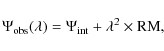
where RM is the Faraday rotation measure. This is related to the magnetic field component along the line-of-sight (B_//) weighted by the thermal gas density (n_e) according to:

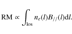
$\begin{displaymath} {\rm RM} \propto \int_{\rm los}n_e(l) B_{//}(l) {\rm d}l. \end{displaymath}$

(2)

Therefore, once the thermal gas density distribution is inferred from X-ray observations, RM studies give an additional set of information about the cluster magnetic field. This is the only way, so far, to study the intracluster magnetic field in clusters where diffuse radio emission sources are not directly observed.

The Coma cluster magnetic field has been studied in the past using all three approaches mentioned above. The first investigation of the magnetic field was performed by Kim et al. (1990). They analyzed 18 bright radio-sources in the Coma cluster region, obtaining RM maps at $\sim$ $20\hbox{$^{\prime\prime}$ }$ ( $\sim$ 9.2 kpc) resolution and found a significant enhancement of the RM in the inner parts of the cluster. Assuming a simple model for the magnetic field reversal length, they derived a field strength of $\sim$ 2 $\mu$ G. A complimentary study was performed by Feretti et al. (1995) studying the polarization properties of the extended radio galaxy NGC 4869. From the average value of RM and its dispersion across the source, they deduced a magnetic field of $\sim$ 6 $\mu$ G tangled on scales of $\sim$ 1 kpc, in addition to a weaker magnetic field component of $\sim$ 0.2 $\mu$ G , uniform on a cluster core radius scale.

From the Coma radio halo, assuming equipartition, a magnetic field estimate of $\sim$ 0.7-1.9 $\mu$ G is derived (Thierbach et al. 2003), while from the Inverse Compton hard X-ray emission a value of $\sim$ 0.2 $\mu$ G has been derived by Fusco Femiano et al. (2004), although new hard X-ray observations performed with a new generation of satellites did not find such evidence of non-thermal emission (Wik et al. 2009, using XMM and Suzaku data, Lutovinov et al. 2008 using ROSAT, RXTE and INTEGRAL data, Ajello et al. 2009, using XMM-Newton, Swift/XRT, Chandra and BAT data; see Sect. 8).

However, the discrepancy between these values is not surprising: equipartition and IC estimates, in fact, rely on several assumptions, and are cluster volume averaged estimates, while the RM is sensitive to the local structures of both the thermal plasma and the cluster magnetic field component that is parallel to the line of sight. Furthermore, the equipartition estimate should be used with caution, given the number of underlying assumptions. For example, it depends on the poorly known particle energy distribution, and in particular on the low energy cut-off of the emitting electrons (see e.g. Beck & Krause 2005).

These different estimates provide direct evidence of the complex structure of the cluster magnetic field and show that magnetic field models where both small and large scale structure coexist must be considered. The intracluster magnetic field power spectrum has been investigated in several works (Vogt & Ensslin 2003, 2005; Murgia et al. 2004; Govoni et al. 2006; Guidetti et al. 2008; Laing et al. 2008). In addition, a radial decline of the magnetic field strength is expected from magneto-hydrodynamical simulations performed with different codes (Dolag et al. 1999, 2005; Brueggen et al. 2005; Dubois et al. 2008; Collins et al. 2010; Dolag & Stasyszyn 2009; Donnert et al. 2009a), as a result of the compression of thermal plasma during the cluster gravitational collapse.

In this paper we present a new study of the Coma cluster magnetic field. We analyzed new Very Large Array (VLA) polarimetric observations of seven sources in the Coma cluster field, and used the FARADAY code developed by Murgia et al. (2004) to derive the magnetic field model that best represents our data through numerical simulations.

The Coma cluster is an important target for a detailed study of cluster magnetic fields. It is a nearby cluster (z=0.023), it hosts large scale radio emission (radio halo, radio relic, bridge) and a wealth of data are available at different energy bands, from radio to hard X-rays.

Table 1: VLA observations of radio galaxies in the Coma cluster field.

The paper is organized as follows: in Sect. 2 the properties of the X-ray emitting gas are described, in Sect. 3 radio observations are presented, and the radio properties of the sources are analyzed. RM analysis is presented in Sect. 4 while in Sect. 5 the adopted magnetic field model is described. The method we adopted to compare simulations and observations is reported in Sect. 6, numerical simulations are presented in Sect. 7 and results are discussed in Sect. 8. Finally, conclusions are reported in Sect. 9.

A $\Lambda$ CDM cosmological model is assumed throughout the paper, with H₀=71 km s^-1 Mpc^-1, $\Omega_{\rm M}=0.27$ , $\Omega_{\Lambda}=0.73$ . This means that 1 arcsec corresponds to 0.460 kpc at z=0.023.

2 Thermal component from X-ray observations

The study of the magnetic field through the Faraday RM requires knowledge of the properties of the thermal gas (see Eq. (2)). This information can be derived from X-ray observations. In Fig. 1 the X-ray emission of the Coma cluster is shown in colors. X-ray observations in the energy band 0.1-2.4 keV have been retrieved from the ROSAT All Sky Survey data archive. After background subtraction the image has been divided by the exposure map and smoothed with a Gaussian of $\sigma=60\hbox{$^{\prime\prime}$ }$ .

The radio contours of the NVSS (NRAO VLA Sky Survey) at 1.4 GHz are overlaid onto the X-ray emission in Fig. 1. The location of the sources studied in this paper are marked with their names. Note that the extended radio emission of the radio halo, relic and bridge are completely resolved out in the NVSS image due to the lack of extremely short baselines.

The X-ray emission is from thermal bremsstrahlung, and can be used to trace the thermal particle distribution in the ICM. The distribution of the gas is well reproduced by the so-called $\lq\lq \beta$ -model'' (Cavaliere & Fusco Femiano 1976), reported in Eq. (3):

$\begin{displaymath}n_e(r)=n_0 \left(1+\frac{r^2}{r^2_{\rm c}}\right)^{-\frac{3}{2}\beta}, \end{displaymath}$

(3)

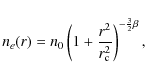
where r indicates the radial distance from the cluster center, $r_{\rm c}$ is the cluster core radius, n₀ is the cluster central gas density. The cluster center is RA = 12 $^{\rm h}$ 59 $^{\rm m}$ 41.5 $^{\rm s}$ ; Dec. = 27 $^{\circ}$ 56 $^{\prime \prime }$ 20 $^{\prime \prime }$ . We use the values derived by Briel et al. (1992), corrected for the cosmology adopted in this paper. They found:

$\beta=0.75\pm 0.03$ ;
$r_{\rm c}=291\pm 17$ kpc;
$n_0=3.44 \pm 0.04 \times 10^{-3}$ cm^-3.

Table 2: Total and polarization intensity radio images. Images are restored with a beam of $1.5\hbox {$^{\prime \prime }$ }\times 1.5\hbox {$^{\prime \prime }$ }$ .

3 Radio observations and images

3.1 VLA observations and data reduction

We selected from NVSS a sample of sources having a peak flux density larger than 45 mJy, located in a radius of $1^{\rm o}$ from the cluster X-ray center center ( $\simeq$ $5 r_{\rm c}$ ), and which have indication of polarization from Kim et al. (1990). A further selection was performed on the basis of the position of the sources. Observations have been performed at the VLA on 7 sources: 5C4.85 (NGC 4874), 5C4.81 (NGC 4869), 5C4.74, 5C4.114, 5C4.127, 5C4.42, and 5C4.152. Radio observations were performed using the 6 cm and 3.6 cm bands for all of the source except 5C4.114. This source being weaker, was observed at 20 cm and 6 cm. The sources were observed at two frequencies within each band, in order to have 4 frequency observations: 4.535 GHz, 4.935 GHz, 8.085 GHz, and 8.465 GHz. In addition 4.735 GHz observations were performed on sources 5C4.85 and 5C4.74. Due to technical issues the observing time for the source 5C4.152 was reduced, and it was necessary to increase the signal-to-noise ratio in the 3.6 cm band. To increase the signal-to-noise ratio, the data at 8.085 and 8.465 GHz were averaged together and a single image at 8.275 GHz was obtained. For the source 5C4.114 we have observations at 1.365 GHz, 1.516 GHz, 4.535 GHz and 4.935 GHz. Details of the observations are reported in Table 1. The source 3C286 was used as both primary flux density calibrator and as absolute reference for the electric vector polarization angle. The source 1310+323 was observed as both a phase and parallactic angle calibrator.

We performed standard calibration and imaging using the NRAO Astronomical Imaging Processing Systems (AIPS). Cycles of phase self-calibration were performed to refine antenna phase solutions on target sources, followed by a final amplitude and gain self-calibration cycle in order to remove minor residual gain variations. Total intensity, I, and Stokes parameter Q and U images have been obtained for each frequency separately. After cleaning, radio images were restored with a naturally weighted beam. The final images were then convolved with a Gaussian beam having ${\it FWHM}= 1.5\hbox{$^{\prime\prime}$ }\times 1.5\hbox{$^{\prime\prime}$ }$ ( $\sim$ 0.7 $\times$ 0.7 kpc). Polarization intensity $P=\sqrt{U^2+Q^2}$ , Polarization angle $\Psi=\frac{1}{2}atan(U,Q)$ and fractional polarization $FPOL=\frac{P}{I}$ images were obtained from the I, Q and U images. Polarization intensity images have been corrected for a positive bias. The calibration errors on the measured fluxes are $\sim$ 5%.

3.2 Radio properties of the observed sources

In this section the radio properties of the observed sources are briefly presented. Further details are given in Table 2.

Redshift information is available for three out of the seven observed radio sources. Two of them (5C4.85 and 5C4.81) are well studied Coma cluster members, while the third one (5C4.127) is associated with a background source. Although the redshift is not known for the other four radio sources, they have not been identified with any cluster member down to very faint optical magnitudes: $M_r \geq -15$ (see Miller et al. 2009). This indicates that they are background radio sources, seen in projection through the cluster. In the following the radio emission arising from the selected sample of sources is described together with their main polarization properties. In the fractional polarization images (from Figs. 2 to 8) pixels with errors larger than 10% were blanked.

5C4.85 - NGC 4874 This a cluster source, optically identified with the Coma central cD galaxy NGC 4874 (see e.g. Mehlert et al. 2000). It is a Wide Angle Tail radio galaxy, whose maximum angular extension is $\sim$ 30 $\hbox {$^{\prime \prime }$ }$ , corresponding to $\sim$ 15 kpc. The angular extension of the two lobes individually is larger at the lowest frequency. The northern lobe shows a mean fractional polarization of 10% and 11% at 4.535 and 8.465 GHz respectively, while the western lobe is less polarized ( $\sim$ 7% at both frequencies). In Fig. 2 the radio emission is shown at 4.535 and 8.465 GHz.

5C4.81 - NGC 4869

This source has been studied in detail by Dallacasa et al. (1989) and Feretti et al. (1995). It is associated with the giant elliptical galaxy NGC 4869. 5C4.81 has a Narrow Angle Tail radio morphology, and its angular size in the images obtained here is 55 $^{\prime \prime }$ (25 kpc). The mean fractional polarization in the tail is 18% at 4.535 GHz and 21% at 8.465 GHz. In Fig. 3 the radio emission is shown at 4.535 and 8.465 GHz.

5C4.74
The source 5C4.74 consists of 5C4.74a and 5C4.74b, the two radio lobes of a FRII radio source. Its redshift is unknown, and no optical identification has been found, either with a Coma cluster member (Miller et al. 2009) nor with a background radio source. From this we conclude that it is a distant background source. The northeastern lobe has a fractional polarization of $\sim$ 28% and 35% respectively at 4.535 and 8.465 GHz, while the southwestern lobe is less polarized ( $\sim$ 19% at 4.535 GHz and $\sim$ 23% at 8.465 GHz).

In Fig. 4 the radio emission is shown at 4.535 and 8.465 GHz.

$\begin{figure} \par\includegraphics[width=15cm,clip]{13696fg2.ps} \end{figure}$

Figure 2:

Source 5C4.85. Total intensity radio contours and polarization vectors at 4.535 GHz ( left) and 8.465 GHz ( right). The bottom contour corresponds to a 3 $\sigma$ noise level, contours are then spaced by a factor of 2. E vectors are superimposed: the orientation indicates the direction of the E field, while the line length is proportional to the fractional polarization intensity (1 $\hbox {$^{\prime \prime }$ }$ corresponding to 10%).

Open with DEXTER

$\begin{figure} \includegraphics[width=15.5cm,clip]{13696fg3.ps} \end{figure}$

Figure 3:

Source 5C4.81. Total intensity radio contours and polarization vectors at 4.535 GHz ( left) and 8.465 GHz ( right). The bottom contour corresponds to a 3 $\sigma$ noise level, and contours are then spaced by a factor of 2. E vectors are superimposed: orientation indicates the direction of the E field, while line length is proportional to the fractional polarization intensity (1 $^{\prime \prime }$ corresponding to 10%).

Open with DEXTER

$\begin{figure} \includegraphics[width=16cm,clip]{13696fg4.ps} \end{figure}$

Figure 4:

Source 5C4.74. Total intensity radio contours and polarization vectors at 4.535 GHz ( left) and 8.465 GHz ( right). The bottom contour corresponds to a 3 $\sigma$ noise level, contours are then spaced by a factor of 2. E vectors are superimposed: the orientation indicates the direction of the E field, while the line length is proportional to the fractional polarization intensity (1 $\hbox {$^{\prime \prime }$ }$ corresponding to 10%).

Open with DEXTER

$\begin{figure} \includegraphics[width=15.5cm,clip]{13696fg5.ps} \end{figure}$

Figure 5:

Source 5C4.114. Total intensity radio contours and polarization vectors at 1.365 GHz ( left) and 4.935 GHz ( right). The bottom contour corresponds to a 3 $\sigma$ noise level, contours are then spaced by a factor of 2. E vectors are superimposed: the orientation indicates the direction of the E field, while the line length is proportional to the fractional polarization intensity (1 $\hbox {$^{\prime \prime }$ }$ corresponding to 10%).

Open with DEXTER

$\begin{figure} \par\includegraphics[width=16cm,clip]{13696fg6.ps} \end{figure}$

Figure 6:

Source 5C4.127. Total intensity radio contours and polarization vectors at 4.535 GHz ( left) and 8.465 GHz ( right). The bottom contour corresponds to a 3 $\sigma$ noise level, contours are then spaced by a factor of 2. E vectors are superimposed: the orientation indicates the direction of the E field, while the line length is proportional to the fractional polarization intensity (1 $\hbox {$^{\prime \prime }$ }$ corresponding to 10%).

Open with DEXTER

$\begin{figure} \par\includegraphics[width=16cm,clip]{13696fg7.ps} \end{figure}$

Figure 7:

Source 5C4.42. Total intensity radio contours and polarization vectors at 4.535 GHz ( left) and 8.465 GHz ( right). The bottom contour corresponds to a 3 $\sigma$ noise level, contours are then spaced by a factor of 2. E vectors are superimposed: the orientation indicates the direction of the E field, while the line length is proportional to the fractional polarization intensity (1 $\hbox {$^{\prime \prime }$ }$ corresponding to 10%).

Open with DEXTER

$\begin{figure} \par\includegraphics[width=14.5cm,clip]{13696fg8.ps} \vspace*{-2mm}\end{figure}$

Figure 8:

Source 5C4.152. Total intensity radio contours and polarization vectors at 4.535 GHz ( left) and 8.465 GHz ( right). The bottom contour corresponds to a 3 $\sigma$ noise level, contours are then spaced by a factor of 2. E vectors are superimposed: the orientation indicates the direction of the E field, while the line length is proportional to the fractional polarization intensity (1 $\hbox {$^{\prime \prime }$ }$ corresponding to 10%).

Open with DEXTER

5C4.114
5C4.114 is a FRI radio source, with angular size of $\sim$ 15 $\hbox {$^{\prime \prime }$ }$ . Its redshift is unknown, and no optical identification either with a Coma cluster galaxy (Miller et al. 2009) nor with a background galaxy has been found, indicating that 5C4.114 has a redshift greater than 0.023. The southern lobe appears brighter than the northern one. The source fractional polarization is $\sim$ 13% at 1.365 GHz and $\sim$ 19% at 4.935 GHz.

In Fig. 5 the radio emission is shown at 1.365 and 4.935 GHz.

5C4.127 5C4.127 is a QSO located at z=1.374(Veron-Cetty & Veron 2001). Observations presented here show that in addition to a bright nucleus the source has a weak extension in the E-W direction of $\sim$ 16 $^{\prime \prime }$ ( $\sim$ 136 kpc) at both of the observing frequency bands. The extended component has a mean fractional polarization of 13% at 4.535 GHz and 14% at 8.465 GHz, while the nucleus is polarized at the 3% level. In Fig. 6 radio contours of the source and polarization vector images are shown.

5C4.42 5C4.42 is a FRII-type radio source. Redshift information is not available in the literature and no optical identification has been found. The same arguments explained above for the source 5C4.74 let us conclude that it is a background radio source. The source is composed by a weakly polarized core and two lobes that extend for $\sim$ 25 $\hbox {$^{\prime \prime }$ }$ in the southwest and northeast directions. The lobes show a mean fractional polarization of $\sim$ 13% at both 4.535 GHz and 8.465 GHz. In Fig. 7 radio contours and vector polarization images of the source are shown.

5C4.152 5C4.152 is a FRII type Radio Galaxy. No redshift is available in the literature for this source. The same arguments explained above for the source 5C4.74 let us conclude that it is a background radio source. It is composed of a core having a fractional polarization of a few percent and two lobes that extend for $\sim$ 28 $\hbox {$^{\prime \prime }$ }$ north-south. The lobes show a mean fractional polarization of $\sim$ $\sim$ 13% 4.535 GHz and 15% at 8.275 GHz. In Fig. 8 radio contours and vector polarization images of the source are shown.

$\begin{figure} \par\includegraphics[width=14.5cm,clip]{13696fg9.eps} \end{figure}$	Figure 9: 5C4.85: Top left: the RM fit is shown in color along with total intensity radio contours 4.935 GHz. The bottom contour correspond to the 3 $\sigma$ noise level and contours are then spaced by a factor of 2. Top right: distribution histogram of the RM values. Bottom: fits of polarization angle versus $\lambda ^2$ in four representative pixels.
Open with DEXTER

$\begin{figure} \par\includegraphics[width=14.5cm,clip]{13696f10.eps} \end{figure}$	Figure 10: 5C4.81: Top left: the RM image is shown in color along with total intensity radio contours at 4.935 GHz. Contours start at 3 $\sigma$ and increase by factors of 2. Top right: distribution histogram of the RM values. Bottom: fits of polarization angle versus $\lambda ^2$ in four representative pixels.
Open with DEXTER

$\begin{figure} \par\includegraphics[width=14.5cm,clip]{13696f11.eps} \end{figure}$	Figure 11: 5C4.74: Top left: the RM image is shown in color along with total intensity radio contours at 4.935 GHz. Contours start at 3 $\sigma$ and increase by factors of 2. Top right: distribution histogram of the RM values. Bottom: fits of polarization angle versus $\lambda ^2$ in four representative pixels.
Open with DEXTER

$\begin{figure} \par\includegraphics[width=14.5cm,clip]{13696f12.eps} \end{figure}$	Figure 12: 5C4.114: Top left: the RM image is shown in colors along with total intensity radio contours at 4.935 GHz. Contours start at 3 $\sigma$ and increase by factors of 2. Top right: distribution histogram of the RM values. Bottom: fits of polarization angle versus $\lambda ^2$ in four representative pixels.
Open with DEXTER

$\begin{figure} \par\includegraphics[width=15cm,clip]{13696f13.eps} \end{figure}$	Figure 13: 5C4.127: Top left: the RM image is shown in color along with total intensity radio contours at 4.935 GHz. Contours start at 3 $\sigma$ and increase by factors of 2. The circle indicates the area masked in the RM analysis. Top right: distribution histogram of the RM values. Bottom: fits of polarization angle versus $\lambda ^2$ in four representative pixels.
Open with DEXTER

$\begin{figure} \par\includegraphics[width=14.5cm,clip]{13696f14.eps} \end{figure}$	Figure 14: 5C4.42: Top left: the RM image is shown in color along with total intensity radio contours at 4.935 GHz. Contours start at 3 $\sigma$ and increase by factors of 2. Top right: distribution histogram of the RM values. Bottom: fits of polarization angle versus $\lambda ^2$ in four representative pixels.
Open with DEXTER

$\begin{figure} \par\includegraphics[width=14.5cm,clip]{13696f15.eps} \end{figure}$	Figure 15: 5C4.152: Top left: the RM image is shown in color along with total intensity radio contours at 4.935 GHz. Contours start at 3 $\sigma$ and increase by factors of 2. Top right: distribution histogram of the RM values. Bottom: fits of polarization angle versus $\lambda ^2$ in four representative pixels.
Open with DEXTER

4 RM: fits and errors

In this section the procedure used to derive the RM from the radio observations is explained. We used the PACERMAN algorithm (Polarization Angle CorrEcting Rotation Measure ANalysis) developed by Dolag et al. (2005). The algorithm solves the n $\pi$ ambiguity in low signal-to-noise regions by exploiting the information of nearby reference pixels, under the assumption that the reference pixel is connected to the nearby areas as far as the polarization angle gradient is below a certain threshold in all of the observed frequency maps simultaneously.

We considered as reference pixel those with a polarization angle uncertainty less than 7 degrees, and fixed the gradient threshold to 15 degrees. An error of 7 degrees in the polarization angle corresponds to 3 $\sigma$ level in both U and Q polarization maps simultaneously. We allowed PACERMAN to perform the RM fit if at least in 3 frequency maps the above mentioned conditions were satisfied. The resulting RM images are shown in Figs. 9-15 overlaid on the total intensity contours at 4.935 GHz. In the same figures we also provide the RM distribution histograms and the RM fits for selected pixels in the map. The linear trend of $\Psi$ versus $\lambda ^2$ and the good fits obtained clearly indicate that the Faraday rotation is occurring in an external screen.

From the RM images we computed the RM mean ( $\langle \rm RM\rangle$ ) and its dispersion ( $\sigma_{\rm RM,obs}$ ). There are two different types of errors that we have to account for: the statistical error and the fit error. The statistical errors for $\langle \rm RM\rangle$ and for $\sigma_{\rm RM,obs}$ is given by $\sigma_{\rm RM,obs}/ \sqrt{n_b}$ and $\sigma_{\rm RM,obs}/ \sqrt{2n_b}$ respectively, where n_b is the number of beams over which the RM has been computed. The statistical error is the dominant one, while the error of the fit has the effect of increasing the real value of $\sigma _{\rm RM}$ . Thus, in order to recover the real standard deviation of the observed RM distribution we have computed the $\sigma_{\rm RM,Dec.}$ as $\sqrt{\sigma^2_{\rm RM,obs}-\rm Median(Err_{fit})^2}$ . with $\rm Median(Err_{fit})$ being the median of the error distribution. The fit error has been estimated with Monte Carlo simulations. We have extracted n_b values, from a random Gaussian distribution having $\sigma=\sigma_{\rm RM,obs}$ and mean $=\langle \rm RM \rangle$ , we have then added to the extracted values a Gaussian noise having $\sigma_{\rm noise}=\rm Err_{\rm fit}$ , in order to mimic the effect of the noise in the observed RM images. We have computed the mean and the dispersion ( $\sigma_{\rm sim}$ ) of these simulated quantities and then subtracted the noise from the dispersion obtaining $\sigma_{\rm sim,De.c}=\sqrt{\sigma_{\rm sim}^2-\sigma_{\rm noise}^2}$ . We have thus obtained a distribution of $\sigma_{\rm sim,Dec.}$ and means. The standard deviation of the $\sigma_{\rm sim,Dec}$ distribution is then the fit error on $\sigma_{\rm RM,Dec.}$ while the standard deviation of the mean distribution is the fit error on $\langle \rm RM\rangle$ . We checked that the mean of both distributions recover the corresponding observed values. In Table 3 we report the RM mean, the observed RM dispersion ( $\sigma_{\rm RM,obs}$ ), the value of $\sigma_{\rm RM,Dec.}$ (hereafter simply $\sigma _{\rm RM}$ ), with the respective errors, the average fit error (Err $_{\rm fit}$ ), and the number of beams over which the RM statistic is computed (n_b).

4.0.1 The source 5C4.74

The value of $\langle \rm RM\rangle$ that we have derived for the source 5C4.74 is quite high compared with the values found for the other sources in this cluster and it is also higher than the values obtained in other clusters for sources at similar distances from the cluster center (e.g. Clarke et al. 2004). The level of polarization of this source is also quite high compared to the other sources (see Sect. 3.2). We note its position southwest of the cluster core, in the direction of the sub-group NGC 4839 that is currently merging with the Coma cluster (Feretti & Neumann 2006). One possibility is that the magnetic field and/or the thermal gas has been compressed and ordered in this region, increasing the observed polarization flux and making $\langle \rm RM\rangle$ peculiar in this position. This might imply that more sophisticated models, that include deviations from a spherical symmetry could give a better representation of the gas density profile. We note however that the X-ray analysis performed in the literature by Briel et al. (1992) shows that the spherical $\beta$ -model is a good representation of the cluster X-ray surface brightness, indicating that deviations from spherical symmetry are small. The $\sigma _{\rm RM}$ value is fully compatible with the trend suggested by the other sources. This could be explained in the proposed scenario, if the magnetic field has been compressed and ordered. In the following analysis we will use mainly the $\sigma _{\rm RM}$ to infer the magnetic field strength and structure. Nonetheless, results will also be presented excluding this source from our analysis.

4.1 Galactic contribution

The contribution to the Faraday RM from our Galaxy may introduce an offset in the Faraday rotation that must be removed. This contribution depends on the galactic positions of the observed sources. The Coma cluster Galactic coordinates are $l=58^{\circ}$ and $b=88^{\circ}$ . The cluster is close to the galactic north pole, so that Galactic contribution to the observed RM is likely negligible. However, in order to estimate this contribution the average RM for extragalactic sources located in projection nearby the Coma cluster region has been computed using the catalogue by Simard-Normadin et al. (1981). The RM from each source have been weighted by the inverse of the distance from the Coma cluster center. It results that in a region of $25\times 25$ degrees² centered on the cluster, the Galactic contribution of $\sim$ -0.15 rad/m². This small contribution is thus completely negligible and has been ignored in the following analysis.

4.2 RM local contribution

We discuss here the possibility that the RM observed in radio galaxies are not associated with the foreground ICM but may arise locally to the radio source (Bicknell et al. 1990; Rudnick & Blundell 2003), either in a thin layer of dense warm gas mixed along the edge of the radio emitting plasma, or in its immediate surroundings. There are several arguments against this interpretation:

the trend of RM versus the cluster impact parameter in both statistical studies and individual cluster investigations (Clarke et al. 2001, 2004; Feretti et al. 1999; Govoni et al. 2005);
the Laing-Garrington effect (Laing 1988; Garrington et al. 1988; Garrington & Conway 1991). This effect consists of an asymmetry in the polarization properties of the lobes of bright radio sources with one-sided, large scale jets. The lobe associated with the jet that is beamed toward the observer is more polarized than the one associated with the counter-jet that points away from the observer. This effect can be explained if we assume that the radio emission from the two lobes cross different distances through the ICM, and therefore the emission from the counter-lobe is seen through a greater Faraday depth, causing greater depolarization. This means also that the observed polarization properties of the source are strongly influenced by the ICM;
statistical tests on the scatter plot of RM versus polarization angle for the radio galaxy PKS1246-410 (Ensslin et al. 2003);
the relation between the RM and the cooling flow rate in relaxed clusters (Taylor et al. 2002).

This observational evidence allows us to conclude that the main contribution to the RM occurs in a Faraday screen located outside the radio sources. The only contribution that could contaminate the cluster Faraday screen is the contribution from the disturbed ISM in the central parsecs of the host elliptical galaxy where the inner jet has been found to have RMs up to thousands of radians per square meter (Zavala & Taylor 2004). We removed the core from the RM analysis in order to avoid any contribution of this kind (out to a distance of $\sim$ 5 $\hbox {$^{\prime \prime }$ }$ from the core).

The ICM origin of the observed RM is also confirmed by the data presented here (Table 3): the trend of $\sigma _{\rm RM}$ exhibits a decrease with increasing cluster impact parameter. Values of $\langle\rm RM\rangle \neq$ 0 and different among sources located at different projected distances to the cluster center indicate that the magnetic field substantially changes on scales larger than the source size, while small RM fluctuation can be explained by magnetic field fluctuation on scales smaller than the source size. Thus in order to interpret correctly the RM data we have to take into account magnetic field fluctuations over a range of spatial scales, i.e., we have to model the magnetic field power spectrum.

Table 3: Rotation measures values of the observed sources.

5 The magnetic field model

In this section the magnetic field model adopted to simulate RM images is described. We used the approach suggested by Murgia et al. (2004), where the magnetic field is modelled as a 3-dimensional multi-scale model and its intensity scales with radius, following the gas distribution.

5.1 The magnetic field power spectrum

In order to study the magnetic field of the Coma cluster, we considered a 3D vectorial magnetic field model.

Simulations start considering a power spectrum for the vector potential $\vec{A}$ in the Fourier domain:

$\begin{displaymath}\vert A_k\vert^2 \propto k^{-\zeta} \end{displaymath}$

(4)

and extract random values of its amplitude A and phase $\phi$ . Ais randomly extracted from a Rayleigh distribution (in order to obtain a Gaussian distribution for the real magnetic field components, as frequently observed), while $\phi$ varies randomly from 0 to 2 $\pi$ . The magnetic field components in the Fourier space are then obtained by:

$\begin{displaymath}{\tilde B}(k) =ik\times {\tilde A}(k). \end{displaymath}$

(5)

The field components B_i in the real space are then derived using 3D Fast Fourier Transform. The resulting magnetic field is a multi-scale model with the following properties:

1)

$\begin{displaymath}\nabla \cdot \vec{B}=0;\end{displaymath}$

2)

the magnetic field energy density associated with each component B_k is:

|B_k|² = C²_n k^-n,

$n= \zeta -2$ , where C²_n is the power spectrum normalization;

3)

B_i has a Gaussian distribution, with $\langle B_i\rangle=0$ , $\sigma_{B_i}=\langle B^2_i\rangle$ ,

4)

B has a Maxwellian distribution.

The magnetic field model scales with the radius as described in Sect. 5.2.

We define $\Lambda=\frac{2\pi}{k}$ as the physical scale of the magnetic field fluctuations in the real space. Thus in order to determine the magnetic field power spectrum in the cluster, we have to determine three parameters: $\Lambda _{\rm min}$ , $\Lambda _{\rm max}$ and n. It is worth noting that a degeneracy arises between $\Lambda _{\rm max}$ and n (the higher n is, the lower $\Lambda _{\rm max}$ is, in order to produce the same RM, see also Sect. 7.1).

5.2 The magnetic field radial profile

There are several indications that the magnetic field intensity decreases going from the center to the periphery of a cluster. This is expected by magneto-hydrodynamical simulations (see e.g. Dolag et al. 2008) and by spatial correlations found in some clusters between thermal and non-thermal energy densities (Govoni et al. 2001).

We assume that the cluster magnetic field follows the thermal component radial distribution according to:

$\begin{displaymath}\langle \vec{B}\rangle(r)= \langle \vec{B}_0\rangle \left( \frac{n_e(r)}{n_0} \right)^{\eta} \end{displaymath}$

(6)

where $\langle \vec{B}_0\rangle$ is the mean magnetic field strength at the cluster center.

In order to obtain the desired magnetic field radial profile we have operated directly in the real space. Strictly, this operation should be performed in the Fourier space, by convolving the spectral potential components with the shaping profile. It has been proved that these two approaches give negligible differences (see Murgia et al. 2004).

When the magnetic field profile is considered, two more parameters have to be determined: $\eta$ and $\langle \vec{B}_0\rangle$ . These two parameters are degenerate (the higher is $\langle \vec{B}_0\rangle$ the higher is $\eta$ ). In fact higher central value of the field require a steeper spectrum in order to produce the same RM.

The adopted magnetic field model has then a total of 5 free parameters: $\Lambda _{\rm min}$ , $\Lambda _{\rm max}$ , n, $\eta$ and $\langle B_0\rangle$ , and is subject to two degeneracies: $\Lambda {_{\rm max}}-{n}$ and $\eta$ and $\langle B_0\rangle$ .

Fitting all of these five parameters simultaneously would be the best way to proceed, but it is not feasible here, due to the computational burden caused by the Fourier Transform inversion. Indeed we have to simulate a large volume $\sim$ 3³ Mpc³ with a sub-kiloparsec pixel-size.

The aim of this work is to constrain the magnetic field radial profile, and for this reason the sources were selected in order to sample different regions at different impact parameters. This allows us to reach a good sensitivity to the RM at different distances from the cluster center.

We proceed as follows: we perform 2D simulations with different magnetic field power spectra in order to recover the RM statistical indicator that are sensitive to the magnetic field power spectrum (Sect. 7.1). From this analysis we derive the power spectrum that best reproduces the observations. We then perform 3D magnetic field simulations varying the values of B₀ and $\eta$ and derive the magnetic field profile that best reproduces the RM observations (Sect. 7.3).

6 Comparing observations and simulations

A tricky point when observations and simulations are compared is the correct evaluations of the errors and uncertainties that this process is subject to. The simulations we present in this paper start from a random seed and generate 2D and 3D magnetic fields. From these fields simulated RM images are obtained, and then compared with those observed in order to constrain the magnetic field properties. It is worth noting that for a given magnetic field model, the RM in a given position of the cluster varies depending on the initial seed of the simulation, so that different realizations of the same model will correspond to different values of $\langle \rm RM\rangle$ and $\sigma _{\rm RM}$ at that position. Given the limited area covered by RM observations, the random nature of the field cannot be neglected in our analysis.

We adopt the following approach to compare observations and simulations: once the simulated RM image is obtained for a source, it is convolved with a Gaussian function having ${\it FWHM}$ equal to the beam ${\it FWHM}$ of the observed image. The simulated RM image is then blanked in the same way as the observed RM image. This ensures that simulations are subject to the same sampling bias that we have to deal with when obtaining the RM from observations. The comparison between the observed RM images and those simulated is performed with the $\chi ^2$ distribution, by computing:

$\begin{displaymath} \chi^2 = \sum^7_{i=1}{\frac{(C_{i,\rm obs} - \langle C_{i,\rm sim} \rangle)^2}{{\rm Err}^2_{C_{i,\rm obs}}}} \end{displaymath}$

(7)

where i indicates the source, $C_{\rm obs}$ refers to a generic observed quantity, while $\langle C_{i,\rm sim}\rangle$ is the same quantity averaged over the different equivalent numerical simulation that start with different random seeds, and ${\rm Err}^2_{C_{i,\rm obs}}$ refers to the error of $C_{\rm obs}$ .

7 Determining the magnetic field from RM observations

Here we describe how the magnetic field power spectrum has been investigated.

7.1 Constraining the magnetic field power spectrum

Several observational quantities can be useful to constrain some properties of the magnetic field power spectrum. In particular:

both $\langle \rm RM\rangle$ and $\sigma _{\rm RM}$ scale linearly with the magnetic field strength, while they have different trends with n and $\Lambda _{\rm max}$ , which are degenerate parameters. The ratio $\vert\langle \rm RM \rangle\vert/\sigma_{\rm RM}$ can thus be used to investigate the magnetic field power spectrum (see also Fig. 3 in Murgia et al. 2004);
the minimum scale of the magnetic field fluctuation, $\Lambda _{\rm min}$ , affects the depolarization ratio (DP ratio) at two different frequencies (i.e. $DP=\frac{P_{\nu_1}/I_{\nu_1}}{P_{\nu_2}/I_{\nu_2}}$ ) and the $\sigma _{\rm RM}$ . Both DP and $\sigma _{\rm RM}$ are in fact determined by the magnetic power on the small spatial scales. This parameter can be thus be derived by studying high resolution polarization images;
It has been demonstrated that the magnetic field auto-correlation function is proportional to the RM auto-correlation function (Ensslin & Vogt 2003). Since the power spectrum is the Fourier transform of the auto-correlation function, it is possible to study the 3D magnetic field power spectrum starting from the power spectrum of the RM images.

We simulated 2D magnetic field models with different power spectra and compared simulated RM images and DP with the corresponding observable quantities. In these simulations the power spectrum normalization is set independently for each source. The computational grid is $512 \times 512$ pixel² and the pixel-size was fixed to 0.2 kpc. This guarantees that each beam is represented by three pixels in the grid. The resulting field of view is then $\sim$ 100 $\times$ 100 kpc², that is enough to recover the projected size of the sources and to properly sample the large power spectrum scales. A Gaussian noise having $sigma=\rm Err_{\rm fit}$ was added to the simulated images. Simulations were finally convolved with a Gaussian function having FMHM equal to the beam of the observations.

7.1.1 The $\Lambda {_{\rm max}}-{n}$ plane

In order to illustrate the degeneracy existing between $\Lambda _{\rm max}$ and n, 2D magnetic field models with different power spectra have been simulated. We allowed the parameter n to vary in the range [0.5;4.5] and $\Lambda _{\rm max}$ in the range [5;600] kpc, with steps of 0.06 and 9.3 kpc respectively. We derived simulated RM images for each combination of these parameters and calculated the RM ratio as:

$\begin{displaymath}{\rm RM}~ {\rm ratio}=\frac{\vert\langle {\rm RM} \rangle\vert } {\sigma_{\rm RM} } \end{displaymath}$

(8)

in a region of $15\times15$ kpc², comparable to the regions where RM has been observed. In Fig. 16 the values of the RM ratio for the simulated RM images is shown in colors, as a function of both n and $\Lambda _{\rm max}$ . The RM ratio was computed for the observed source that have a RM signal-to noise ratio >3 both for $\sigma _{\rm RM}$ and $\langle \rm RM\rangle$ , i.e for the sources 5C4.85, 5C4.81, 5C4.74 and 5C4.114. The resulting values are shown in Fig. 16 (black line).

The plot in Fig. 16 shows what $\Lambda {_{\rm max}}-{n}$ degeneracy means: the same value of the RM ratio can be explained with different power spectra. There are, as expected, two asymptotic trends. In fact, if the magnetic field power spectrum is flat (e.g. n<3), the bulk of the magnetic field energy is on the small scales, and thus the effect of increasing $\Lambda _{\rm max}$ is negligible after a certain threshold, that in this case is achieved for $\Lambda_{\rm max}\sim 300$ kpc. As the power spectrum steepens, as n>3 the bulk of the energy moves to large scales, and thus as $\Lambda _{\rm max}$ increases, the energy content also increases sharply. This is the reason of the second asymptotic trend that is shown in the plot: as n increases $\Lambda _{\rm max}$ decreases faster and faster. As n approaches the value of $\sim$ 11/3 (Kolmogorov power spectrum), the observed data constrain $\Lambda _{\rm max}$ to be $\sim$ 20-40 kpc.

7.2 Structure function, auto-correlation function and multi-scale-statistic

In order to constrain more precisely the estimate of the magnetic field power spectrum parameters indicated by the previous analysis we have investigated the statistical properties of the RM images individually. We have fixed n=11/3, corresponding to the Kolmogorov power law for turbulent fields. This choice is motivated by both observational and theoretical works. Schuecker et al. (2004) analyzed spatially-resolved gas pseudo-pressure maps of the Coma galaxy cluster deriving that pressure fluctuations in the cluster center are consistent with a Kolmogorov-like power spectrum. Furthermore, cosmological numerical simulations have recently demonstrated that 3D power spectrum of the velocity field is well described by a single power law out to at least one virial radius, with a slope very close to the Kolmogorov power law (Vazza et al. 2009a,b).

The range of values of $\Lambda _{\rm max}$ is suggested by the previous analysis (see Fig. 16). In order to choose the best parameters in that range, and to find the best value for $\Lambda _{\rm min}$ , we simulated RM images and used two different statistical methods to compare the observed RM images to the simulated ones:

1.

we calculated the auto-correlation function and the structure function of the observed RM images, and then compared them with the simulated RM images. The RM structure function is defined as follows.

$\begin{displaymath}S({\rm d}x,{\rm d}y)=\left\langle \left[{\rm RM}(x,y)-{\rm RM}(x+{\rm d}x,y+{\rm d}y)\right]^2\right\rangle_{(x,y)}, \end{displaymath}$

(9)

where $=\langle \rangle_{(x,y)}$ indicates that the average is taken over all the positions (x,y) in the RM image. Blank pixels were not considered in the statistics. The structure function S(r) is then computed by radially averaging $S({\rm d}x,{\rm d}y)$ over regions of increasing size of radius $r=\sqrt{{\rm d}x^2+{\rm d}y^2}$ . S(r) is thus sensitive to the observable quantity $\sigma _{\rm RM}$ over different scales. The auto-correlation function is defined as:

$\begin{displaymath}A({\rm d}x,{\rm d}y)=\langle [{\rm RM}(x,y) {\rm RM}(x+{\rm d}x,y+{\rm d}y)]\rangle_{(x,y)} \end{displaymath}$

(10)

Since $A(0)=\langle {\rm RM}^2 \rangle=\sigma^2_{\rm RM}+\langle {\rm RM} \rangle^2$ , the auto-correlation function is sensitive to both $\langle \rm RM\rangle$ and the $\sigma _{\rm RM}$ .

2.

We computed a Multi-Scale Statistic (MSS), namely we computed $\langle \rm RM\rangle$ and $\sigma _{\rm RM}$ over regions of increasing size in the observed RM images and compared them with the same values obtained in the simulated images. The smallest region over which $\langle \rm RM\rangle$ and $\sigma _{\rm RM}$ are computed corresponds to a box of $0.4 \times 0.4$ kpc size. The box side is then increased by a factor two until the full source size is reached. We note that this approach is sensitive to both $\langle \rm RM\rangle$ and $\sigma _{\rm RM}$ over different spatial scales, and is thus a useful tool to discriminate among different power spectra. This indicator differs from the S(r) and A(r) in that as r increases, the number of pixels useful for computing the multi-scale statistic increases, giving a robust statistical estimate on large scales.

For each source we simulated different power spectra varying $\Lambda _{\rm min}$ from 1 kpc to 5 kpc and $\Lambda _{\rm max}$ from 20 to 40 kpc. For every power spectrum and for each source we realized ten different 2D RM images, and compared the statistics (S(r), A(r) and MSS) with the observed ones by computing Eq. (7). This approach makes it possible to discriminate the best power spectrum model compatible with our data. In this 2D analysis we focused on the sources 5C4.85, 5C4.81, 5C4.74 and 5C4.114, whose RM images have signal-to-noise ratio >3. Each source was fitted separately. The total $\chi ^2$ was then computed by summing the individual values obtained for each source. The minimum value of the total $\chi^2_{\rm tot}$ corresponds to the power spectrum model characterized by $\Lambda _{\rm max}=34$ kpc and $\Lambda _{\rm min}=2$ kpc. We show in Figs. 17 and 18 the structure function, auto-correlation function and multi-scale statistics for the Kolmogorov power spectrum model that best reproduces the observed RM images. In Appendix A similar Figures obtained with other power spectrum models are shown.

$\begin{figure} \par\includegraphics[width=8cm,clip]{13696f16.eps} \end{figure}$	Figure 16: The RM ratio $\vert\langle \rm RM \rangle\vert/\sigma_{\rm RM}$ as a function of n and $\Lambda _{\rm max}$ computed on simulated RM images. The line refers to the mean values obtained by averaging the ratio of the sources.
Open with DEXTER

$\begin{figure} \par\includegraphics[width=17cm,clip]{13696f17.ps} \end{figure}$

Figure 17:

Fits to the RM images for the Kolmogorov power spectrum that best reproduces the observed RM (n=11/3, $\Lambda _{\rm min}=2$ kpc, $\Lambda _{\rm max}=34$ kpc) globally for the sources used in the 2D analysis (see Sect. 7.1). From top to bottom: fit to the $\sigma _{\rm RM}$ and $\langle \rm RM\rangle$ . Red diamonds represent the observed statistic, the cyan line represents the mean taken over ten different realizations of the same magnetic field power spectrum, and the blue lines represent the scatter in the simulations.

Open with DEXTER

$\begin{figure} \par\includegraphics[width=17cm,clip]{13696f18.ps} \end{figure}$

Figure 18:

Fits to the RM images for the Kolmogorov power spectrum that best reproduces the observed RM (n=11/3, $\Lambda _{\rm min}=2$ kpc, $\Lambda _{\rm max}=34$ kpc) globally for the sources used in the 2D analysis (see Sect. 7.1). Fit to the S(r) ( top) and A(r) ( bottom). Red diamonds represent the observed statistic, the cyan line represents the mean taken over ten different realizations of the same magnetic field power spectrum, and the blue lines represent the scatter in the simulations.

Open with DEXTER

7.2.1 $\Lambda _{\rm min}$ and fractional polarization

It has been demonstrated (Burn 1966, see also Laing 2008) that when Faraday rotation occurs the fractional polarization FPOL can be related to the fourth power of the observing wavelength $\lambda$ according to the Burn law:

$\begin{displaymath} {\rm FPOL}=\frac{P_{\lambda}}{I_{\lambda}}\propto \exp\left(-k \lambda^4\right). \end{displaymath}$

(11)

Since FPOL is sensitive to the minimum scale of the power spectrum, $\Lambda _{\rm min}$ , Eq. (11) can be used to constrain it. We fitted Eq. (11) to our observations and to our simulations, performed with different values of $\Lambda _{\rm min}$ . These fits indicate that a Kolmogorov power spectrum with the best agreement with observations is achieved for $\Lambda_{\rm min}\sim2$ kpc, confirming the result from the previous analysis. As an example, we show in Fig. 19 these fits performed on the source 5C4.114, where the effect of depolarization is more appreciable, thanks to the 20 cm observations.

7.3 The magnetic field profile

The results obtained from the previous section indicate the power spectrum that is able to best reproduce the observed RM images. In order to investigate the magnetic field radial profile we simulated 3D Kolmogorov power spectra, with $\Lambda _{\rm max}=34$ kpc and $\Lambda _{\rm min}=2$ kpc, as derived from the 2D analysis (Sect. 7.1). A computational grid of 2048³ pixels was used, and the pixel-size was fixed to 0.5 kpc. This guarantees that the Nyquist criteria is satisfied for $\Lambda _{\rm min}$ and that fluctuations on scales $\sim$ $\Lambda _{\rm max}$ are also well represented in the cube. For each of these simulations Eq. (2) was integrated numerically, with a step of 0.5 kpc along the line of sight. The limits of the integral in Eq. (2) were $[0; 10 r_{\rm c}]$ for the cluster's sources 5C4.85 and 5C4.81 and $[-10 r_{\rm c}; 10 r_{\rm c}]$ for the other sources in the background of the cluster. The simulated field of view covers an area of 1024 $\times$ 1024 kpc², thus the cube has been replicated to achieve a field of view that is large enough to reach the farthest source (5C4.152).

The integration was repeated by varying the parameter B₀ in the range [0.1; 11] $\mu$ G, with a step of $\sim$ 0.17 $\mu$ G, and $\eta$ in the range[-0.2; 2.5] with a step of 0.04. For each combination of B₀and $\eta$ a RM simulated image was thus obtained covering the full cluster area.

We extracted from this RM image seven fields, each lying in the plane of the sky in the same position of the observed sources, and having the same size of the observed RM images. The simulated RM images were convolved with a Gaussian beam having ${\it FWHM}=0.7\times 0.7$ kpc, in order to have the same resolution of the observations. Finally the simulated RM fields were blanked in the same way as the corresponding observed RM images.

The result of this integration is, for each combination of (B₀; $\eta$ ), a set of seven simulated RM images, that are subject to the same statistical biases of the observed images.

This process was repeated 50 times, each starting from a different random seed to generate the magnetic field power spectrum model.

For each source and for each pair of values (B₀; $\eta$ ) a simulated RM image was obtained for every realization of the same power spectrum model. The mean and the standard deviation of the $\sigma_{\rm RM,sim}(B_0,\eta)$ was computed from the simulated RM images, and then the $\chi ^2$ was obtained (Eq. (7)). The resulting $\chi ^2$ plane is shown in Fig. 20. The minimum value is achieved for B₀=4.7 $\mu$ G and $\eta=0.5$ , but the 1- $\sigma$ confidence level of the $\chi ^2$ indicates that values going from B₀=3.9 $\mu$ G and $\eta=0.4$ , to B₀=5.4 $\mu$ G and $\eta=0.7$ , are equally representative of the magnetic field profile, according to the degeneracy between the two parameters. Magnetic field models with a profile flatter than $\eta < 0.2$ and steeper than $\eta > 1.0$ are excluded at 99% confidence level, for any value of $\langle B_0\rangle$ . Also magnetic field models with $\langle B_0 \rangle < 3.1~\mu$ G and $\langle B_0 \rangle > 6.5$ $\mu$ G are excluded at the 99% confidence level for any value of $\eta$ . It is interesting to note that the best models include $\eta=0.5$ , the value expected in the case of a magnetic field energy density decreasing in proportion to the gas energy density (assuming a constant average gas temperature), and $\eta=0.67$ , expected in the case of a magnetic field frozen into the gas. In the latter case the corresponding value of $\langle B_0\rangle$ is $\sim$ 5.2 $\mu$ G.

The knowledge of the magnetic field strength and structure in the ICM has strong implications for models explaining the formation of diffuse radio sources like radio halos. Testing the different models proposed in the literature is beyond the scope of this paper. We point out, however, that cosmological simulations recently performed by Donnert et al. (2009b) have shown that it is possible to test a class of these models once the magnetic field profile is known.

7.4 Results excluding the source 5C4.74

The same procedure described above has been repeated excluding the source 5C4.74 (see Sect. 4.0.1). The minimum value for the $\chi ^2$ is again achieved with a model characterized by B₀=4.7 $\mu$ G and $\eta=0.5$ . This is not surprising since the fit is computed based on $\sigma _{\rm RM}$ , and the source is sampled with only 10 beams. In order to investigate possible effects arising from the interaction of the Coma cluster with the NGC 4839 group RM images of more sources in this region would be required.

$\begin{figure} \par\includegraphics[width=8.5cm,clip]{13696f19.ps} \end{figure}$	Figure 19: Fits to the Burn law. Points refer to observed data, while the red line is the fit obtained from observations. Dashed lines refer to the fits obtained from three different models, with different values of $\Lambda _{\rm min}$ , as reported in the bottom left corner of the plot.
Open with DEXTER

8 Comparison with other estimates

In the literature there is a long-standing debate on the magnetic field strength derived from the RM analysis compared to the equipartition estimate and to the Inverse Compton hard X-ray emission. The discrepancy may arise from the different (but not incompatible) assumptions, and, moreover, are sensitive to the magnetic field on different spatial scales. Assuming the magnetic field models derived in the previous section, it is possible to derive an estimate that is comparable with equipartition values, and with the Inverse-Compton detection as well as with the upper limits derived from new hard X-ray observations. In order to obtain a value that is directly comparable with the equipartition magnetic field estimate, we have to derive the average magnetic field strength resulting from our RM analysis over the same volume assumed in the equipartition analysis, that is $\sim$ 1 Mpc³. The magnetic field model resulting from our RM analysis gives an average magnetic field strength of $\sim$ 2 $\mu$ G, consistent with the equipartition estimate derived from the radio halo emission (0.7-1.9 $\mu$ G Thierbach et al. 2003), despite the different assumptions that these two methods require.

The Inverse Compton hard X-ray emission has been observed with the Beppo Sax satellite. Its field of view is $\sim$ $1.3^{\circ}$ , corresponding to $\sim$ $2.2 \times 2.2$ Mpc² at the Coma redshift. We computed the average value of the magnetic field over the same volume sampled by Beppo Sax. We obtained $\sim$ 0.75 $\mu$ G when the best model is assumed, that is a factor four higher than the value derived from Hard-X ray observations (Fusco Femiano et al. 2004). We note however that models compatible with our data within 1- $\sigma$ of the $\chi ^2$ give values slightly different, going from 0.9 to 0.5 $\mu$ G. The steepest magnetic field model that is compatible with our data at 99% confidence level ( $B_{0}\sim 6.4$ $\mu$ G, $\eta=0.95$ ) gives 0.2 $\mu$ G when averaged over the volume corresponding to the Beppo Sax field of view. Deeper Hard-X ray observations would be required to better compare the two estimates. The values computed here indicate however that they can be reconciled. Recently, new hard X-ray observations of the Coma cluster have been performed with the new generation of satellites (see the work by Wik et al. 2009, using XMM and Suzaku data, Lutovinov et al. 2008, using ROSAT, RXTE and INTEGRAL data, Ajello et al. 2009, using XMM-Newton, Swift/XRT, Chandra and BAT data). These observations failed to find statistically significant evidence for non-thermal emission in the hard X-ray spectrum of the ICM, which is better described by a single or multi-temperature model. Given the large angular size of the Coma cluster, if the non-thermal hard X-ray emission is more spatially extended than the observed radio halo, both Suzaku HXD-PIN and BAT Swift may miss some fraction of the emission. These efforts have thus derived lower limits for the magnetic field strength, over areas smaller than the radio halo. The lower limit reported by Wik et al. (2009) is e.g. $\langle B \rangle > 0.2$ $\mu$ G, that is compatible with our results.

$\begin{figure} \par\includegraphics[width=17.5cm,clip]{13696f20.ps} \vspace*{-2mm}\end{figure}$	Figure 20: Left: $\chi ^2$ plane obtained by comparing simulated and observed $\sigma _{\rm RM}$ . Right: profile of the best magnetic field model. magenta line refers to the analytic profile (Eq. (6)), while the blue line refers to a slice extracted from the simulated magnetic field numerical model. Power spectrum fluctuations on the profile are shown.
Open with DEXTER

9 Conclusions

We have presented new VLA observations of seven sources in the Coma cluster field at multiple frequencies in the range 1.365-8.465 GHz. The high resolution of these observations has allowed us to obtained detailed RM images with 0.7 kpc resolution. The sources were chosen in order to sample different lines-of-sight in the Coma cluster in order to constrain the magnetic field profile. We used the numerical approach proposed by Murgia et al. (2004) to realize 3D magnetic field models with different central intensities and radial slopes, and derived several realizations of the same magnetic field model in order to account for any possible effect deriving from the random nature of the magnetic field. Simulated RM images were obtained, and observational biases such as noise, beam convolution and limited sampled regions were all considered in comparing models with the data. We found that $\sigma _{\rm RM}$ and $\langle \rm RM\rangle$ decrease with increasing distance from the cluster center, except for the source 5C4.74, that shows a high value of $\langle \rm RM\rangle$ . We argue that this may arise from its peculiar position southwest of the Coma cluster core, toward the NGC4839 group that is currently merging with the Coma cluster.

Our results can be summarized as follows:

the RM ratio and the DP ratio were used to analyze the magnetic field power spectrum. Once a Kolmogorov index is assumed, the structure-function, the auto-correlation function and the multi-scale statistic of the RM images are best reproduced by a model with $\Lambda _{\rm max}=34$ kpc and $\Lambda _{\rm min}=2$ kpc. We performed a further check to investigate the best value of $\Lambda _{\rm min}$ by fitting the Burn law (Burn 1966). This confirmed the result obtained from the previous analysis.
The magnetic field radial profile was investigated through a series of 3D simulations. By comparing the observed and simulated $\sigma _{\rm RM}$ values we find that the best models are in the range (B₀=3.9 $\mu$ G; $\eta=0.4$ ) and (B₀=5.4 $\mu$ G; $\eta=0.7$ ). It is interesting to note that the values $\eta=0.5$ and 0.67 lie in this range. They correspond to models where the magnetic field energy density scales as the gas energy density, or the magnetic field is frozen into the gas, respectively. This is expected from a theoretical point-of-view since the energy in the magnetic component of the intracluster medium is a tiny fraction of the thermal energy. Values of B₀>7 $\mu$ G and <3 $\mu$ G as well as $\eta < 0.2$ and $\eta > 1.0$ are incompatible with RM data at the 99% confidence level.

The average magnetic field intensity over a volume of $\sim$ 1 Mpc³ is $\sim$ 2 $\mu$ G, and can be compared with the equipartition estimate derived from the radio halo emission. Although based on different assumptions, and although the many uncertainties relying under the equipartition estimate, the model derived from RM analysis gives an average estimate that is compatible with the equipartition estimate. A direct comparison with the magnetic field estimate derived from the IC emission is more difficult, since the Hard-X detection is debated, and depending on the particle energy spectrum, the region over which the IC emission arises may change. The model derived from RM analysis gives a magnetic field estimate that is consistent with the present lower limits obtained from hard X-ray observations. The values we obtain for our best models are still a bit higher when compared with the estimate given by Fusco Femiano et al. (2004).

$\begin{figure} \par\includegraphics[width=7.5cm,clip]{13696f21.ps} \end{figure}$	Figure 21: $\sigma _{\rm RM}$ and $\langle \rm RM\rangle$ for the best model (cyan continuous line) and its dispersion (cyan dotted lines), given by the rms of the different random realizations. Observed points are shown in red.
Open with DEXTER

It is worth to remind, as noted by several authors (see Sec. 8), that the IC estimate derived from Hard X-ray observations could be dominated by the outer part of the cluster volume, where the magnetic field intensity is lower, depending on the spatial and energy distribution of the emitting particles. Future Hard-X ray missions could help in clarifying this issue.

Acknowledgements

A.B. is grateful to the people at the Osservatorio Astronomico di Cagliari for their kind hospitality. We thank R. Fusco Femiano and G. Brunetti for useful discussions. This work is part of the ``Cybersar'' Project, which is managed by the COSMOLAB Regional Consortium with the financial support of the Italian Ministry of University and Research (MUR), in the context of the ''Piano Operativo Nazionale Ricerca Scientifica, Sviluppo Tecnologico, Alta Formazione (PON 2000-2006)''. K. D. acknowledges the supported by the DFG Priority Programme 117. NRAO is a facility of the National Science Fundation, operated under cooperative agreement by Associated Universities. This work was partly supported by the Italian Space Agency (ASI), and by the Italian Ministry for University and research (MIUR). This research has made use of the NASA/IPAC Extragalactic Data Base (NED) which is operated by the JPL, California institute of Technology, under contract with the National Aeronautics and Space Administration.

Appendix A: Structure function and multi-scale statistics with different power spectrum models

In this Appendix we discuss how other power-law spectral models could be representative of the data presented in the paper. The analysis is performed on the basis of the the structure-function, auto-correlation function and multi-scale statistics. Following the approach discussed in Sect. 7.1, we have obtained simulated RM images from different power spectrum models and compared them with observed data. We show in Fig. A.1 the structure function, auto-correlation function and MSS for Kolmogorov power spectra that differ in the value of $\Lambda _{\rm max}$ . We show in Fig. A.2 the fit to the structure, auto-correlation functions and MSS for power spectrum models with n=2, and different values of $\Lambda _{\rm max}$ . We show only the plots obtained for the central source 5C4.85. These figures demonstrate how the RM data presented in this paper are sensitive to different power spectrum models.

We note that Kolmogorov power spectra with $\Lambda_{\rm max}\sim 100$ and 10 kpc fail in reproducing the $\langle \rm RM\rangle$ . These trends can be easily understood since power spectrum models with n>3 have most of the magnetic energy on large spatial scales, and thus small changes in $\Lambda _{\rm max}$ have a consistent impact on the resulting statistics. According to results presented in Sect. 7.1.1, the case $\Lambda_{\rm max}=20$ kpc gives a reasonable fit to our data, although the best fit is achieved for $\Lambda _{\rm max}=34$ kpc. In Fig. A.2 similar fits obtained for power spectra models with n=2 are shown. As indicated by the analysis performed in Sect. 7.1.1, in this case the best agreement with observations is achieved for $\Lambda _{\rm max}$ of order of hundreds kpc (Fig. 16). We note that because of the power spectrum degeneracy, it is possible to obtain a reasonable fit to our data. Indeed the case $\Lambda_{\rm max}=400$ -800 kpc can reproduce the MSS statistics, although they fail in reproducing the S(r) trend on large spatial scales, indicating that a larger value of n is required.

$\begin{figure} \par\includegraphics[width=15cm,clip,clip]{13696f22.ps} \vspace*{-3mm}\end{figure}$

Figure A.1:

Fit to the RM images for different Kolmogorov power spectra for the central sources 5C4.85. The different models are indicated by different colors (see labels) left: fit to the $\sigma _{\rm RM}$ and $\langle \rm RM\rangle$ ; right: fit to the S(r) and A(r). Red diamonds represent the observed statistics. Lines represent the value obtained by averaging 10 power spectra generated with different random seeds.

Open with DEXTER

$\begin{figure} \par\includegraphics[width=15cm,clip]{13696f23.ps} \end{figure}$

Figure A.2:

Fit to the RM images for different power spectra with n=2 for the central sources 5C4.85. The different models are indicated by different colors (see labels) left: fit to the $\sigma _{\rm RM}$ and $\langle \rm RM\rangle$ ; right: fit to the S(r) and A(r). Red diamonds represent the observed statistics. Lines represent the value obtained by averaging 10 power spectra generated with different random seeds.

Open with DEXTER

Appendix B: Limits on the magnetic field profile from background radio sources.

Although several arguments (see Sect. 4.2) suggest that the main contribution to the observed RMs is due to the ICM, the best way to firmly avoid any kind of local contribution would be to consider only background radio galaxies in the analysis. This is however not trivial in general and not feasible here. In fact, sources located in the inner region of the cluster, at distances $\leq$ $(1{-}2) r_{\rm C}$ are fundamental to constrain the magnetic field strength and radial decline, so that a peculiar cluster where background bright and wide sources are seen in projection very close to the cluster center would be required. These conditions are not fulfilled in the case of the Coma cluster, even though it is a very nearby cluster, where several lines of sight can be inspected. We show in Fig. B.1 (left panel) the $\chi ^2$ plane obtained by considering only the background radio galaxies: 5C4.74, 5C4.114, 5C4.127, 5C4.42 and 5C4.152. This plot shows that for every value of B₀ it is possible to find a value of $\eta$ that can reproduce the observed data within 1- $\sigma$ confidence level. In the same figure in the right panel we show the trends of $\sigma _{\rm RM}$ and $\langle \rm RM\rangle$ as a function of r obtained for different value of B₀. They all lie within 1 $\sigma$ confidence level of the $\chi ^2$ plane. It is clear from this plot that the missing information at projected distances r < 300 kpc does not permit us to infer the magnetic field strength and radial decline in the Coma cluster. Even unrealistic models where $\eta\leq0$ cannot be ruled out when the two wide central sources are not considered. Future instruments such as SKA are expected to detect many more radio sources seen through a single cluster, possibly allowing this kind of analysis to be performed excluding cluster members.

$\begin{figure} \par\includegraphics[width=15.5cm,clip]{13696f24.ps} \end{figure}$	Figure B.1: Left: $\chi ^2$ plane obtained by comparing simulated and observed $\sigma _{\rm RM}$ for background sources. Lines refer to 1, 2 and 3- $\sigma$ confidence level. Right: $\sigma _{\rm RM}$ and $\langle \rm RM\rangle$ trends for different models that lie within 1- $\sigma$ confidence level of the $\chi ^2$ .
Open with DEXTER

References

Ajello, M., Rebusco, P., Cappelluti, N., et al. 2009, ApJ, 690, 367 [NASA ADS] [CrossRef] [Google Scholar]
Beck, R., & Krause, M. 2005, AN, 326, 414 [Google Scholar]
Bicknell, G. V., Cameron, R. A., & Gingold, R. A. 1990, ApJ, 357, 373 [NASA ADS] [CrossRef] [Google Scholar]
Briel, U. G., Henry, J. P., & Boehringer, H. 1992, A&A, 259, L31 [NASA ADS] [Google Scholar]
Brüggen, M., Ruszkowski, M., Simionescu, A., Hoeft, M., & Dalla Vecchia, C. 2005, ApJ, 631, L21 [NASA ADS] [CrossRef] [Google Scholar]
Burn, B. J. 1966, MNRAS, 133, 67 [NASA ADS] [CrossRef] [Google Scholar]
Cavaliere, A., & Fusco-Femiano, R. 1976, A&A, 49, 137 [NASA ADS] [Google Scholar]
Clarke, T. E. 2004, JKAS, 37, 337 [NASA ADS] [Google Scholar]
Clarke, T. E., Kronberg, P. P., & Böhringer, H. 2001, ApJ, 547, L111 [NASA ADS] [CrossRef] [Google Scholar]
Collins, D. C., Xu, H., Norman, M. L., Li, H., & Li, S. 2010, ApJS, 186, 308 [NASA ADS] [CrossRef] [Google Scholar]
Dallacasa, D., Feretti, L., Giovannini, G., & Venturi, T. 1989, A&AS, 79, 391 [NASA ADS] [Google Scholar]
Dolag, K. 2006, AN, 327, 575 [NASA ADS] [CrossRef] [Google Scholar]
Dolag, K., & Stasyszyn, F. A. 2009, MNRAS, 398, 1678 [NASA ADS] [CrossRef] [Google Scholar]
Dolag, K., Schindler, S., Govoni, F., & Feretti, L. 2001, A&A, 378, 777 [NASA ADS] [CrossRef] [EDP Sciences] [Google Scholar]
Dolag, K., Bartelmann, M., & Lesch, H. 2002, A&A, 387, 383 [NASA ADS] [CrossRef] [EDP Sciences] [Google Scholar]
Dolag, K., Vogt, C., & Enßlin, T. A. 2005, MNRAS, 358, 726 [NASA ADS] [CrossRef] [Google Scholar]
Dolag, K., Bykov, A. M., & Diaferio, A. 2008, SSRv, 134, 311 [Google Scholar]
Donnert, J., Dolag, K., Lesch, H., & Müller, E. 2009, MNRAS, 392, 1008 [NASA ADS] [CrossRef] [Google Scholar]
Donnert, J., Dolag, K., Brunetti, G., Cassano, R., & Bonafede, A. 2010, MNRAS, 401, 47 [NASA ADS] [CrossRef] [Google Scholar]
Dubois, Y., & Teyssier, R. 2008, A&A, 482, L13 [NASA ADS] [CrossRef] [EDP Sciences] [Google Scholar]
Ensslin, T. A., Vogt, C., Clarke, T. E., & Taylor, G. B. 2003, ApJ, 597, 870 [NASA ADS] [CrossRef] [Google Scholar]
Feretti, L., & Neumann, D. M. 2006, A&A, 450, L21 [NASA ADS] [CrossRef] [EDP Sciences] [Google Scholar]
Feretti, L., Dallacasa, D., Giovannini, G., Tagliani, A. 1995, A&A, 302, 680 [NASA ADS] [Google Scholar]
Feretti, L., Dallacasa, D., Govoni, F., et al. 1999, A&A, 344, 472 [NASA ADS] [Google Scholar]
Ferrari, C., Govoni, F., Schindler, S., Bykov, A. M., & Rephaeli, Y. 2008, SSRv, 134, 93 [Google Scholar]
Fusco-Femiano, R. 2004, Ap&SS, 294, 37 [NASA ADS] [CrossRef] [Google Scholar]
Fusco-Femiano, R., Orlandini, M., Brunetti, G., et al. 2004, ApJ, 602L, 73 [Google Scholar]
Garrington, S. T., & Conway, R. G. 1991, MNRAS, 250, 198 [NASA ADS] [Google Scholar]
Garrington, S. T., Leahy, J. P., Conway, R. G., & Laing, R. A. 1988, Nature, 331, 147 [NASA ADS] [CrossRef] [Google Scholar]
Giovannini, G., & Feretti, L. 2004, J. Korean Astron. Soc., Proceedings of the 3rd Korean Astrophysics Workshop, Cosmic Rays and Magnetic Fields in Large Scale Structure, Pusan, Korea, August 2004, ed. H. Kang, & D. Ryu, 37, 1 [Google Scholar]
Giovannini, G., Bonafede, A., Feretti, L., et al. 2009, A&A, 507, 1257 [NASA ADS] [CrossRef] [EDP Sciences] [Google Scholar]
Govoni, F., Murgia, M., Feretti, L., et al. 2005, A&A, 430, L5 [NASA ADS] [CrossRef] [EDP Sciences] [Google Scholar]
Govoni, F., Murgia, M., Feretti, L., et al. 2006, A&A, 460, 425 [NASA ADS] [CrossRef] [EDP Sciences] [Google Scholar]
Guidetti, D., Murgia, M., Govoni, F., et al. 2008, A&A, 483, 699 [NASA ADS] [CrossRef] [EDP Sciences] [Google Scholar]
Laing, R. A. 1988, Nature, 331, 149 [NASA ADS] [CrossRef] [Google Scholar]
Laing, R. A., Bridle, A. H., Parma, P., & Murgia, M. 2008, MNRAS, 391, 521 [NASA ADS] [CrossRef] [Google Scholar]
Lutovinov, A. A., Vikhlinin, A., Churazov, E. M., Revnivtsev, M. G., & Sunyaev, R. A. 2008, ApJ, 687, 968 [NASA ADS] [CrossRef] [Google Scholar]
Mehlert, D., Saglia, R. P., Bender, R., & Wegner, G. 2000, A&AS, 141, 449 [NASA ADS] [CrossRef] [EDP Sciences] [Google Scholar]
Miller, N. A., Hornschemeier, A. E., Mobasher, B., et al. 2009, AJ, 137, 4450 [NASA ADS] [CrossRef] [Google Scholar]
Murgia, M., Govoni, F., Feretti, L., et al. 2004, A&A, 424, 429 [NASA ADS] [CrossRef] [EDP Sciences] [Google Scholar]
Kim, K. T., Kronberg, P. P., Dewdney, P. E., & Landecker, T. L. 1990, ApJ, 335, 29 [NASA ADS] [CrossRef] [Google Scholar]
Rudnick, L., & Blundell, K. M. 2003, ApJ, 588, 143 [NASA ADS] [CrossRef] [Google Scholar]
Schuecker, P., Finoguenov, A., Miniati, F., Böhringer, H., & Briel, U. G. 2004, A&A, 426, 387 [NASA ADS] [CrossRef] [EDP Sciences] [Google Scholar]
Simard-Normandin, M., Kronberg, P. P., & Button, S. 1981, ApJS, 45, 97 [NASA ADS] [CrossRef] [Google Scholar]
Taylor, G. B., Fabian, A. C., & Allen, S. W. 2002, MNRAS, 334, 769 [NASA ADS] [CrossRef] [Google Scholar]
Thierbach, M., Klein, U., & Wielebinski, R. 2003, A&A, 397, 53 [NASA ADS] [CrossRef] [EDP Sciences] [Google Scholar]
Vazza, F., Brunetti, G., Kritsuk, A., et al. 2009, A&A, 504, 33 [NASA ADS] [CrossRef] [EDP Sciences] [Google Scholar]
Vazza, F., Gheller, C., & Brunetti, G. 2010, A&A, 513, A32 [NASA ADS] [CrossRef] [EDP Sciences] [Google Scholar]
Venturi, T., Giacintucci, S., Dallacasa, D., et al. 2008, A&A, 484, 327 [NASA ADS] [CrossRef] [EDP Sciences] [Google Scholar]
Véron-Cetty, M.-P., & Véron, P. 2001, A&A, 374, 92 [NASA ADS] [CrossRef] [EDP Sciences] [Google Scholar]
Vogt, C., & Enßlin, T. A. 2003, A&A, 412, 373 [NASA ADS] [CrossRef] [EDP Sciences] [Google Scholar]
Vogt, C., & Enßlin, T. A. 2005, A&A, 434, 67 [NASA ADS] [CrossRef] [EDP Sciences] [Google Scholar]
Wik, D. R., Sarazin, C. L., Finoguenov, A., et al. 2009, ApJ, 696, 1700 [NASA ADS] [CrossRef] [Google Scholar]

Footnotes

... calibrator: We refer to the flux density scale by Baars et al. (1990).
... source: In these 2D RM simulations the radial profile of the magnetic field is not accounted for. This implicitly assumes that the mean magnetic field strength is not dramatically varying over the scale of the source. This is a reasonable assumption since the linear sizes of the sources at the Coma redshift are in fact much smaller that the cluster core radius.

All Tables

Table 1: VLA observations of radio galaxies in the Coma cluster field.

Table 2: Total and polarization intensity radio images. Images are restored with a beam of $1.5\hbox {$^{\prime \prime }$ }\times 1.5\hbox {$^{\prime \prime }$ }$ .

Table 3: Rotation measures values of the observed sources.

All Figures

$\begin{figure} \par\includegraphics[width=12cm,clip]{13696fg1.ps} \end{figure}$	Figure 1: Colors: Coma X-ray emission from the ROSAT All Sky Survey in the energy band [0.1, 2.4] kev. Contours: Coma radio emission at 1.4 GHz from the NVSS. The beam FWHM is $45\hbox {$^{\prime \prime }$ }\times 45\hbox {$^{\prime \prime }$ }$ , contours start from 1.5 mJy/beam and are spaced by a factor of 2. The observed sources are labelled.
Open with DEXTER
In the text

$\begin{figure} \par\includegraphics[width=15cm,clip]{13696fg2.ps} \end{figure}$	Figure 2: Source 5C4.85. Total intensity radio contours and polarization vectors at 4.535 GHz ( left) and 8.465 GHz ( right). The bottom contour corresponds to a 3 $\sigma$ noise level, contours are then spaced by a factor of 2. E vectors are superimposed: the orientation indicates the direction of the E field, while the line length is proportional to the fractional polarization intensity (1 $\hbox {$^{\prime \prime }$ }$ corresponding to 10%).
Open with DEXTER
In the text

$\begin{figure} \includegraphics[width=15.5cm,clip]{13696fg3.ps} \end{figure}$	Figure 3: Source 5C4.81. Total intensity radio contours and polarization vectors at 4.535 GHz ( left) and 8.465 GHz ( right). The bottom contour corresponds to a 3 $\sigma$ noise level, and contours are then spaced by a factor of 2. E vectors are superimposed: orientation indicates the direction of the E field, while line length is proportional to the fractional polarization intensity (1 $^{\prime \prime }$ corresponding to 10%).
Open with DEXTER
In the text

$\begin{figure} \includegraphics[width=16cm,clip]{13696fg4.ps} \end{figure}$	Figure 4: Source 5C4.74. Total intensity radio contours and polarization vectors at 4.535 GHz ( left) and 8.465 GHz ( right). The bottom contour corresponds to a 3 $\sigma$ noise level, contours are then spaced by a factor of 2. E vectors are superimposed: the orientation indicates the direction of the E field, while the line length is proportional to the fractional polarization intensity (1 $\hbox {$^{\prime \prime }$ }$ corresponding to 10%).
Open with DEXTER
In the text

$\begin{figure} \includegraphics[width=15.5cm,clip]{13696fg5.ps} \end{figure}$	Figure 5: Source 5C4.114. Total intensity radio contours and polarization vectors at 1.365 GHz ( left) and 4.935 GHz ( right). The bottom contour corresponds to a 3 $\sigma$ noise level, contours are then spaced by a factor of 2. E vectors are superimposed: the orientation indicates the direction of the E field, while the line length is proportional to the fractional polarization intensity (1 $\hbox {$^{\prime \prime }$ }$ corresponding to 10%).
Open with DEXTER
In the text

$\begin{figure} \par\includegraphics[width=16cm,clip]{13696fg6.ps} \end{figure}$	Figure 6: Source 5C4.127. Total intensity radio contours and polarization vectors at 4.535 GHz ( left) and 8.465 GHz ( right). The bottom contour corresponds to a 3 $\sigma$ noise level, contours are then spaced by a factor of 2. E vectors are superimposed: the orientation indicates the direction of the E field, while the line length is proportional to the fractional polarization intensity (1 $\hbox {$^{\prime \prime }$ }$ corresponding to 10%).
Open with DEXTER
In the text

$\begin{figure} \par\includegraphics[width=16cm,clip]{13696fg7.ps} \end{figure}$	Figure 7: Source 5C4.42. Total intensity radio contours and polarization vectors at 4.535 GHz ( left) and 8.465 GHz ( right). The bottom contour corresponds to a 3 $\sigma$ noise level, contours are then spaced by a factor of 2. E vectors are superimposed: the orientation indicates the direction of the E field, while the line length is proportional to the fractional polarization intensity (1 $\hbox {$^{\prime \prime }$ }$ corresponding to 10%).
Open with DEXTER
In the text

$\begin{figure} \par\includegraphics[width=14.5cm,clip]{13696fg8.ps} \vspace*{-2mm}\end{figure}$	Figure 8: Source 5C4.152. Total intensity radio contours and polarization vectors at 4.535 GHz ( left) and 8.465 GHz ( right). The bottom contour corresponds to a 3 $\sigma$ noise level, contours are then spaced by a factor of 2. E vectors are superimposed: the orientation indicates the direction of the E field, while the line length is proportional to the fractional polarization intensity (1 $\hbox {$^{\prime \prime }$ }$ corresponding to 10%).
Open with DEXTER
In the text

$\begin{figure} \par\includegraphics[width=14.5cm,clip]{13696fg9.eps} \end{figure}$	Figure 9: 5C4.85: Top left: the RM fit is shown in color along with total intensity radio contours 4.935 GHz. The bottom contour correspond to the 3 $\sigma$ noise level and contours are then spaced by a factor of 2. Top right: distribution histogram of the RM values. Bottom: fits of polarization angle versus $\lambda ^2$ in four representative pixels.
Open with DEXTER
In the text

$\begin{figure} \par\includegraphics[width=14.5cm,clip]{13696f10.eps} \end{figure}$	Figure 10: 5C4.81: Top left: the RM image is shown in color along with total intensity radio contours at 4.935 GHz. Contours start at 3 $\sigma$ and increase by factors of 2. Top right: distribution histogram of the RM values. Bottom: fits of polarization angle versus $\lambda ^2$ in four representative pixels.
Open with DEXTER
In the text

$\begin{figure} \par\includegraphics[width=14.5cm,clip]{13696f11.eps} \end{figure}$	Figure 11: 5C4.74: Top left: the RM image is shown in color along with total intensity radio contours at 4.935 GHz. Contours start at 3 $\sigma$ and increase by factors of 2. Top right: distribution histogram of the RM values. Bottom: fits of polarization angle versus $\lambda ^2$ in four representative pixels.
Open with DEXTER
In the text

$\begin{figure} \par\includegraphics[width=14.5cm,clip]{13696f12.eps} \end{figure}$	Figure 12: 5C4.114: Top left: the RM image is shown in colors along with total intensity radio contours at 4.935 GHz. Contours start at 3 $\sigma$ and increase by factors of 2. Top right: distribution histogram of the RM values. Bottom: fits of polarization angle versus $\lambda ^2$ in four representative pixels.
Open with DEXTER
In the text

$\begin{figure} \par\includegraphics[width=15cm,clip]{13696f13.eps} \end{figure}$	Figure 13: 5C4.127: Top left: the RM image is shown in color along with total intensity radio contours at 4.935 GHz. Contours start at 3 $\sigma$ and increase by factors of 2. The circle indicates the area masked in the RM analysis. Top right: distribution histogram of the RM values. Bottom: fits of polarization angle versus $\lambda ^2$ in four representative pixels.
Open with DEXTER
In the text

$\begin{figure} \par\includegraphics[width=14.5cm,clip]{13696f14.eps} \end{figure}$	Figure 14: 5C4.42: Top left: the RM image is shown in color along with total intensity radio contours at 4.935 GHz. Contours start at 3 $\sigma$ and increase by factors of 2. Top right: distribution histogram of the RM values. Bottom: fits of polarization angle versus $\lambda ^2$ in four representative pixels.
Open with DEXTER
In the text

$\begin{figure} \par\includegraphics[width=14.5cm,clip]{13696f15.eps} \end{figure}$	Figure 15: 5C4.152: Top left: the RM image is shown in color along with total intensity radio contours at 4.935 GHz. Contours start at 3 $\sigma$ and increase by factors of 2. Top right: distribution histogram of the RM values. Bottom: fits of polarization angle versus $\lambda ^2$ in four representative pixels.
Open with DEXTER
In the text

$\begin{figure} \par\includegraphics[width=8cm,clip]{13696f16.eps} \end{figure}$	Figure 16: The RM ratio $\vert\langle \rm RM \rangle\vert/\sigma_{\rm RM}$ as a function of n and $\Lambda _{\rm max}$ computed on simulated RM images. The line refers to the mean values obtained by averaging the ratio of the sources.
Open with DEXTER
In the text

$\begin{figure} \par\includegraphics[width=17cm,clip]{13696f17.ps} \end{figure}$	Figure 17: Fits to the RM images for the Kolmogorov power spectrum that best reproduces the observed RM (n=11/3, $\Lambda _{\rm min}=2$ kpc, $\Lambda _{\rm max}=34$ kpc) globally for the sources used in the 2D analysis (see Sect. 7.1). From top to bottom: fit to the $\sigma _{\rm RM}$ and $\langle \rm RM\rangle$ . Red diamonds represent the observed statistic, the cyan line represents the mean taken over ten different realizations of the same magnetic field power spectrum, and the blue lines represent the scatter in the simulations.
Open with DEXTER
In the text

$\begin{figure} \par\includegraphics[width=17cm,clip]{13696f18.ps} \end{figure}$	Figure 18: Fits to the RM images for the Kolmogorov power spectrum that best reproduces the observed RM (n=11/3, $\Lambda _{\rm min}=2$ kpc, $\Lambda _{\rm max}=34$ kpc) globally for the sources used in the 2D analysis (see Sect. 7.1). Fit to the S(r) ( top) and A(r) ( bottom). Red diamonds represent the observed statistic, the cyan line represents the mean taken over ten different realizations of the same magnetic field power spectrum, and the blue lines represent the scatter in the simulations.
Open with DEXTER
In the text

$\begin{figure} \par\includegraphics[width=8.5cm,clip]{13696f19.ps} \end{figure}$	Figure 19: Fits to the Burn law. Points refer to observed data, while the red line is the fit obtained from observations. Dashed lines refer to the fits obtained from three different models, with different values of $\Lambda _{\rm min}$ , as reported in the bottom left corner of the plot.
Open with DEXTER
In the text

$\begin{figure} \par\includegraphics[width=17.5cm,clip]{13696f20.ps} \vspace*{-2mm}\end{figure}$	Figure 20: Left: $\chi ^2$ plane obtained by comparing simulated and observed $\sigma _{\rm RM}$ . Right: profile of the best magnetic field model. magenta line refers to the analytic profile (Eq. (6)), while the blue line refers to a slice extracted from the simulated magnetic field numerical model. Power spectrum fluctuations on the profile are shown.
Open with DEXTER
In the text

$\begin{figure} \par\includegraphics[width=7.5cm,clip]{13696f21.ps} \end{figure}$	Figure 21: $\sigma _{\rm RM}$ and $\langle \rm RM\rangle$ for the best model (cyan continuous line) and its dispersion (cyan dotted lines), given by the rms of the different random realizations. Observed points are shown in red.
Open with DEXTER
In the text

$\begin{figure} \par\includegraphics[width=15cm,clip,clip]{13696f22.ps} \vspace*{-3mm}\end{figure}$	Figure A.1: Fit to the RM images for different Kolmogorov power spectra for the central sources 5C4.85. The different models are indicated by different colors (see labels) left: fit to the $\sigma _{\rm RM}$ and $\langle \rm RM\rangle$ ; right: fit to the S(r) and A(r). Red diamonds represent the observed statistics. Lines represent the value obtained by averaging 10 power spectra generated with different random seeds.
Open with DEXTER
In the text

$\begin{figure} \par\includegraphics[width=15cm,clip]{13696f23.ps} \end{figure}$	Figure A.2: Fit to the RM images for different power spectra with n=2 for the central sources 5C4.85. The different models are indicated by different colors (see labels) left: fit to the $\sigma _{\rm RM}$ and $\langle \rm RM\rangle$ ; right: fit to the S(r) and A(r). Red diamonds represent the observed statistics. Lines represent the value obtained by averaging 10 power spectra generated with different random seeds.
Open with DEXTER
In the text

$\begin{figure} \par\includegraphics[width=15.5cm,clip]{13696f24.ps} \end{figure}$	Figure B.1: Left: $\chi ^2$ plane obtained by comparing simulated and observed $\sigma _{\rm RM}$ for background sources. Lines refer to 1, 2 and 3- $\sigma$ confidence level. Right: $\sigma _{\rm RM}$ and $\langle \rm RM\rangle$ trends for different models that lie within 1- $\sigma$ confidence level of the $\chi ^2$ .
Open with DEXTER
In the text

Current usage metrics show cumulative count of Article Views (full-text article views including HTML views, PDF and ePub downloads, according to the available data) and Abstracts Views on Vision4Press platform.

Data correspond to usage on the plateform after 2015. The current usage metrics is available 48-96 hours after online publication and is updated daily on week days.

Initial download of the metrics may take a while.

[1] Ajello, M., Rebusco, P., Cappelluti, N., et al. 2009, ApJ, 690, 367 [NASA ADS] [CrossRef] [Google Scholar]

[2] Beck, R., & Krause, M. 2005, AN, 326, 414 [Google Scholar]

[3] Bicknell, G. V., Cameron, R. A., & Gingold, R. A. 1990, ApJ, 357, 373 [NASA ADS] [CrossRef] [Google Scholar]

[4] Briel, U. G., Henry, J. P., & Boehringer, H. 1992, A&A, 259, L31 [NASA ADS] [Google Scholar]

[5] Brüggen, M., Ruszkowski, M., Simionescu, A., Hoeft, M., & Dalla Vecchia, C. 2005, ApJ, 631, L21 [NASA ADS] [CrossRef] [Google Scholar]

[6] Burn, B. J. 1966, MNRAS, 133, 67 [NASA ADS] [CrossRef] [Google Scholar]

[7] Cavaliere, A., & Fusco-Femiano, R. 1976, A&A, 49, 137 [NASA ADS] [Google Scholar]

[8] Clarke, T. E. 2004, JKAS, 37, 337 [NASA ADS] [Google Scholar]

[9] Clarke, T. E., Kronberg, P. P., & Böhringer, H. 2001, ApJ, 547, L111 [NASA ADS] [CrossRef] [Google Scholar]

[10] Collins, D. C., Xu, H., Norman, M. L., Li, H., & Li, S. 2010, ApJS, 186, 308 [NASA ADS] [CrossRef] [Google Scholar]

[11] Dallacasa, D., Feretti, L., Giovannini, G., & Venturi, T. 1989, A&AS, 79, 391 [NASA ADS] [Google Scholar]

[12] Dolag, K. 2006, AN, 327, 575 [NASA ADS] [CrossRef] [Google Scholar]

[13] Dolag, K., & Stasyszyn, F. A. 2009, MNRAS, 398, 1678 [NASA ADS] [CrossRef] [Google Scholar]

[14] Dolag, K., Schindler, S., Govoni, F., & Feretti, L. 2001, A&A, 378, 777 [NASA ADS] [CrossRef] [EDP Sciences] [Google Scholar]

[15] Dolag, K., Bartelmann, M., & Lesch, H. 2002, A&A, 387, 383 [NASA ADS] [CrossRef] [EDP Sciences] [Google Scholar]

[16] Dolag, K., Vogt, C., & Enßlin, T. A. 2005, MNRAS, 358, 726 [NASA ADS] [CrossRef] [Google Scholar]

[17] Dolag, K., Bykov, A. M., & Diaferio, A. 2008, SSRv, 134, 311 [Google Scholar]

[18] Donnert, J., Dolag, K., Lesch, H., & Müller, E. 2009, MNRAS, 392, 1008 [NASA ADS] [CrossRef] [Google Scholar]

[19] Donnert, J., Dolag, K., Brunetti, G., Cassano, R., & Bonafede, A. 2010, MNRAS, 401, 47 [NASA ADS] [CrossRef] [Google Scholar]

[20] Dubois, Y., & Teyssier, R. 2008, A&A, 482, L13 [NASA ADS] [CrossRef] [EDP Sciences] [Google Scholar]

[21] Ensslin, T. A., Vogt, C., Clarke, T. E., & Taylor, G. B. 2003, ApJ, 597, 870 [NASA ADS] [CrossRef] [Google Scholar]

[22] Feretti, L., & Neumann, D. M. 2006, A&A, 450, L21 [NASA ADS] [CrossRef] [EDP Sciences] [Google Scholar]

[23] Feretti, L., Dallacasa, D., Giovannini, G., Tagliani, A. 1995, A&A, 302, 680 [NASA ADS] [Google Scholar]

[24] Feretti, L., Dallacasa, D., Govoni, F., et al. 1999, A&A, 344, 472 [NASA ADS] [Google Scholar]

[25] Ferrari, C., Govoni, F., Schindler, S., Bykov, A. M., & Rephaeli, Y. 2008, SSRv, 134, 93 [Google Scholar]

[26] Fusco-Femiano, R. 2004, Ap&SS, 294, 37 [NASA ADS] [CrossRef] [Google Scholar]

[27] Fusco-Femiano, R., Orlandini, M., Brunetti, G., et al. 2004, ApJ, 602L, 73 [Google Scholar]

[28] Garrington, S. T., & Conway, R. G. 1991, MNRAS, 250, 198 [NASA ADS] [Google Scholar]

[29] Garrington, S. T., Leahy, J. P., Conway, R. G., & Laing, R. A. 1988, Nature, 331, 147 [NASA ADS] [CrossRef] [Google Scholar]

[30] Giovannini, G., & Feretti, L. 2004, J. Korean Astron. Soc., Proceedings of the 3rd Korean Astrophysics Workshop, Cosmic Rays and Magnetic Fields in Large Scale Structure, Pusan, Korea, August 2004, ed. H. Kang, & D. Ryu, 37, 1 [Google Scholar]

[31] Giovannini, G., Bonafede, A., Feretti, L., et al. 2009, A&A, 507, 1257 [NASA ADS] [CrossRef] [EDP Sciences] [Google Scholar]

[32] Govoni, F., Murgia, M., Feretti, L., et al. 2005, A&A, 430, L5 [NASA ADS] [CrossRef] [EDP Sciences] [Google Scholar]

[33] Govoni, F., Murgia, M., Feretti, L., et al. 2006, A&A, 460, 425 [NASA ADS] [CrossRef] [EDP Sciences] [Google Scholar]

[34] Guidetti, D., Murgia, M., Govoni, F., et al. 2008, A&A, 483, 699 [NASA ADS] [CrossRef] [EDP Sciences] [Google Scholar]

[35] Laing, R. A. 1988, Nature, 331, 149 [NASA ADS] [CrossRef] [Google Scholar]

[36] Laing, R. A., Bridle, A. H., Parma, P., & Murgia, M. 2008, MNRAS, 391, 521 [NASA ADS] [CrossRef] [Google Scholar]

[37] Lutovinov, A. A., Vikhlinin, A., Churazov, E. M., Revnivtsev, M. G., & Sunyaev, R. A. 2008, ApJ, 687, 968 [NASA ADS] [CrossRef] [Google Scholar]

[38] Mehlert, D., Saglia, R. P., Bender, R., & Wegner, G. 2000, A&AS, 141, 449 [NASA ADS] [CrossRef] [EDP Sciences] [Google Scholar]

[39] Miller, N. A., Hornschemeier, A. E., Mobasher, B., et al. 2009, AJ, 137, 4450 [NASA ADS] [CrossRef] [Google Scholar]

[40] Murgia, M., Govoni, F., Feretti, L., et al. 2004, A&A, 424, 429 [NASA ADS] [CrossRef] [EDP Sciences] [Google Scholar]

[41] Kim, K. T., Kronberg, P. P., Dewdney, P. E., & Landecker, T. L. 1990, ApJ, 335, 29 [NASA ADS] [CrossRef] [Google Scholar]

[42] Rudnick, L., & Blundell, K. M. 2003, ApJ, 588, 143 [NASA ADS] [CrossRef] [Google Scholar]

[43] Schuecker, P., Finoguenov, A., Miniati, F., Böhringer, H., & Briel, U. G. 2004, A&A, 426, 387 [NASA ADS] [CrossRef] [EDP Sciences] [Google Scholar]

[44] Simard-Normandin, M., Kronberg, P. P., & Button, S. 1981, ApJS, 45, 97 [NASA ADS] [CrossRef] [Google Scholar]

[45] Taylor, G. B., Fabian, A. C., & Allen, S. W. 2002, MNRAS, 334, 769 [NASA ADS] [CrossRef] [Google Scholar]

[46] Thierbach, M., Klein, U., & Wielebinski, R. 2003, A&A, 397, 53 [NASA ADS] [CrossRef] [EDP Sciences] [Google Scholar]

[47] Vazza, F., Brunetti, G., Kritsuk, A., et al. 2009, A&A, 504, 33 [NASA ADS] [CrossRef] [EDP Sciences] [Google Scholar]

[48] Vazza, F., Gheller, C., & Brunetti, G. 2010, A&A, 513, A32 [NASA ADS] [CrossRef] [EDP Sciences] [Google Scholar]

[49] Venturi, T., Giacintucci, S., Dallacasa, D., et al. 2008, A&A, 484, 327 [NASA ADS] [CrossRef] [EDP Sciences] [Google Scholar]

[50] Véron-Cetty, M.-P., & Véron, P. 2001, A&A, 374, 92 [NASA ADS] [CrossRef] [EDP Sciences] [Google Scholar]

[51] Vogt, C., & Enßlin, T. A. 2003, A&A, 412, 373 [NASA ADS] [CrossRef] [EDP Sciences] [Google Scholar]

[52] Vogt, C., & Enßlin, T. A. 2005, A&A, 434, 67 [NASA ADS] [CrossRef] [EDP Sciences] [Google Scholar]

[53] Wik, D. R., Sarazin, C. L., Finoguenov, A., et al. 2009, ApJ, 696, 1700 [NASA ADS] [CrossRef] [Google Scholar]

The Coma cluster magnetic field from Faraday rotation measures

1 Introduction

2 Thermal component from X-ray observations

3 Radio observations and images

3.1 VLA observations and data reduction

3.2 Radio properties of the observed sources

4 RM: fits and errors

4.0.1 The source 5C4.74

4.1 Galactic contribution

4.2 RM local contribution

5 The magnetic field model

5.1 The magnetic field power spectrum

5.2 The magnetic field radial profile

6 Comparing observations and simulations

7 Determining the magnetic field from RM observations

7.1 Constraining the magnetic field power spectrum

7.1.1 The plane

7.2 Structure function, auto-correlation function and multi-scale-statistic

7.2.1 and fractional polarization

7.3 The magnetic field profile

7.4 Results excluding the source 5C4.74

8 Comparison with other estimates

9 Conclusions

Appendix A: Structure function and multi-scale statistics with different power spectrum models

Appendix B: Limits on the magnetic field profile from background radio sources.

References

Footnotes

All Tables

All Figures

7.1.1 The $\Lambda {_{\rm max}}-{n}$ plane

7.2.1 $\Lambda _{\rm min}$ and fractional polarization