| Issue |
A&A
Volume 513, April 2010
|
|
|---|---|---|
| Article Number | A48 | |
| Number of page(s) | 7 | |
| Section | The Sun | |
| DOI | https://doi.org/10.1051/0004-6361/200913193 | |
| Published online | 23 April 2010 | |
Solar active regions: a nonparametric statistical analysis
J. Pelt1 - M. J. Korpi2,3 - I. Tuominen2
1 - Tartu Observatory, 61602 Tõravere, Estonia
2 -
Observatory, PO Box 14, 00014 University of Helsinki, Finland
3 -
NORDITA, AlbaNova University Center, Roslagstullsbacken 23, 10691 Stockholm, Sweden
Received 27 August 2009 / Accepted 1 February 2010
Abstract
Context. The sunspots and other solar activity indicators
tend to cluster on the surface of the Sun. These clusters very often
occur at certain longitudes that persist in time. It is of general
interest to find new and simple ways to characterize the observed
distributions of different indicators and their behaviour in time.
Aims. In the present work we use Greenwich sunspot data to
evaluate the statistical but not totally coherent stability of the
sunspot distribution along latitudes as well as longitudes. The aim was
to obtain information on the longitudinal distribution of the
underlying spot-generating mechanism rather than on the distribution
and migration of sunspots or sunspot groups on the solar surface.
Therefore only sunspot groups were included in the analysis, and only
the time of their first appearance was used.
Methods. We used a simple nonparametric approach to reveal sunspot migration patterns and their persistency.
Results. Our analysis shows that regions where spots are
generated tend to rotate differentially as the spots and spot groups
themselves do. The spatial correlations in activity, however, tend to
break down relatively fast, during 7-15 solar rotations.
Conclusions. This study provides a challenge for solar dynamo
models, as our results indicate that the non-axisymmetric
spot-generating mechanism experiences differential rotation (known as
phase mixing in dynamo theory). The new nonparametric method introduced
here, completely independent of the choice of the longitudinal
distribution of sunspots, was found to be a useful tool for
spatio-temporal analysis of surface features.
Key words: Sun: activity - magnetic fields - sunspots - methods: statistical
1 Introduction
Modern observations of the Sun are so rich in detail that astronomers are eventually facing an embarrassment of riches. When spatio-temporal properties of the smaller features - say spots, flares, etc. - are treated with well-established vigour, the analysis of spatially larger or temporarily longer patterns is very complicated. Even the nomenclature of the phenomena is not well established - for instance the time-space cluster of the local phenomena can be called ``active longitude'' (Losh 1938; Vitinskij 1969), ``Sonnefleckenherd'' (``flock of sunspots'', Becker 1955), ``active region'' (Bumba & Howard 1965), ``sunspot nest'' (Castenmiller et al. 1986), ``complex of activity'' (Gaizauskas et al. 1983) or ``hot spot'' (Bai 1988). There is, in addition, a problem with the proper definition of such extended patterns.It is generally thought that the tracers of solar activity - sunpots, flares, etc. - are randomly generated manifestations of the larger scale mean magnetic field of the Sun generated by a hydromagnetic dynamo process. An analogy with a submerged animal blowing out bubbles is quite appropriate in this context (see Bai 2003). What can we tell about the swimming speed and size of the animal, if only random bubbles are observable? How deep in water is the animal?
The answers to these kinds of questions depend very much on the method of analysis used. Very often subjective judgement is involved, either through steps of visual processing or through involvement of freely chosen procedure parameters (bin sizes, number of longitudinal modes, detection limits, preselection criteria etc.).
From the statistical analysis point of view we can divide the previously used methods along two lines: how the input data is transformed before computing final statistics and what kind of statistics are used. Some typical but random examples:
- aggregated data (daily Wolf numbers) and correlation analysis (Bogart 1982);
- raw heliographic longitudes and longitude-wise binning (Trotter & Billings 1962; Warwick 1965);
- transformed (using trial rotation velocity) longitudes and
 statistic (Bai 1987);
- transformed (using latitude-dependent rotation velocities) longitudes and pattern matching (Usoskin et al. 2005; Pelt et al. 2006, hereafter PBKT);
- spherical harmonic decomposition and time series analysis of mode amplitudes, phases and phase-walks (Juckett 2003).
We try here to return to the square one in a certain sense, back to the very basics. By very simple considerations and avoiding all freely chosen parameters we try to get answers to these questions:
- is there a tendency for surface elements to occur at certain longitudes that persist over time?
- how are this persistence and the differential rotation of the surface elements connected?
- how long do typical correlations in activity persist?
2 Method of analysis
2.1 Nonparametric method
Let us assume that we have two sets of longitudes:
![]() and
and
![]() .
Their values belong to the interval
.
Their values belong to the interval
![]() and we assume that N<=M (if otherwise, we can
always swap the sets).
We aim to characterize the similarity or
the difference between the two longitude distributions somehow.
The general theory
of directional measurements is considered in mathematical statistics
(see for instance the latest monograph by Mardia & Jupp 2000, and
references therein), but here we need a more specific method, namely one without
any underlying statistical assumptions or parametric models for
the distributions involved.
and we assume that N<=M (if otherwise, we can
always swap the sets).
We aim to characterize the similarity or
the difference between the two longitude distributions somehow.
The general theory
of directional measurements is considered in mathematical statistics
(see for instance the latest monograph by Mardia & Jupp 2000, and
references therein), but here we need a more specific method, namely one without
any underlying statistical assumptions or parametric models for
the distributions involved.
We propose the following very simple nonparametric method:
The circular distance between two longitudes ![]() and
and ![]() we define as usually done
we define as usually done
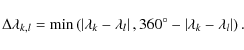
|
(1) |
Let us take a particular longitude
For the particular set sizes N and M we can compute the mathematical
expectation of ![]() for completely random distributions of
longitudes in both sets. Let us denote this expectation as
for completely random distributions of
longitudes in both sets. Let us denote this expectation as
![]() .
Our final statistic, which measures the statistical distance
between the two sets of longitudes, is then
.
Our final statistic, which measures the statistical distance
between the two sets of longitudes, is then
| (2) |
If we wish to stress that the distance D is computed for two particular indexed longitude sets, say for index n (N longitudes) and index m (M longitudes) we use the notation
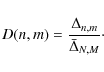
|
(3) |
The mathematical expectations
It is quite obvious that for absolutely random pairs of longitude sets our distance will have a value around 1. For weakly correlated sets values are less than 1, and values higher than 1 can occur when the longitude sets involved are constrained in a certain way due to which they cannot form all the patterns that occur for randomly generated sets. For sunspot groups, for instance, the distributions are constrained by group sizes. Randomly generated points can fall arbitrarily close, which is not true for sunspot longitudes, because for them the group centres are separated by definition.
Now that we have the statistic to measure distances between different
distributions of longitudes we can go further. For a sequence of
longitude sets counted by k we can compute a mean distance between neighbouring
sets
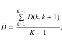
|
(4) |
where K is the number of the sets. We can also investigate how the distance depends on the mutual positions of particular sets
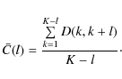
|
(5) |
Obviously
2.2 Rotation and frames
Heliographic longitudes are measured using the so called Carrington frame,
which rotates against fixed stars with the exact period of
![]() days. The mean rotation period if observed from the Earth is
PO=27.2753 days. The Carrington frame is a formal construct and
real features on the Sun need not follow it exactly.
days. The mean rotation period if observed from the Earth is
PO=27.2753 days. The Carrington frame is a formal construct and
real features on the Sun need not follow it exactly.
Let us fix
a certain longitude
![]() of a
particular persistent feature on the Sun rotating with the Carrington
angular velocity. Then its longitude for different Carrington
rotations i will be fixed:
of a
particular persistent feature on the Sun rotating with the Carrington
angular velocity. Then its longitude for different Carrington
rotations i will be fixed:
![]() ,
angular brackets
denoting here and below reduction to the interval
,
angular brackets
denoting here and below reduction to the interval
![]() .
Because the
angular velocity of the Carrington frame is
.
Because the
angular velocity of the Carrington frame is
![]() degrees per day, we can rewrite the cycle-dependent
sequence of longitudes as
degrees per day, we can rewrite the cycle-dependent
sequence of longitudes as
![\begin{displaymath}%
\lambda_i^{(C)} = \left[ {\lambda^{(C)} + i \times \Omega _{\rm C} P_{\rm C} } \right], \quad i = 0,1, \ldots
\end{displaymath}](/articles/aa/full_html/2010/05/aa13193-09/img31.png)
|
(6) |
The actual angular velocity of an arbitrary feature on the Sun need not to be exactly
| (7) |
The corrected frame rotates against the Carrington frame with an angular velocity of
Below we measure the angular velocity in degrees per day, latitude in degrees, and periods in days, and give the values in these units.
2.3 Algorithms
To analyse different frames and the corresponding distributions of modified longitudes we use the statistics described above.
As an input data we take a set of time-tagged longitudes
![]() ,
amounting to L
items of data.
Using the time points tl we divide the records
into subintervals with the length 27.2753 (Carrington rotations). This
procedure is not absolutely exact because the observation timing
depends on the somewhat excentric orbit of the Earth. Fortunately the
errors involved are small and we can ignore them. From the point of
generality and objectivity our choice is quite natural. Historical
observations are all done from Earth and consequently the features can
be observed only half the time. However, during the Carrington rotation
we can record what happens at all longitudes. As far as timing is
considered, due to the rotation some processes can actually start
earlier than observed. This excludes short-lived processes (shorter
than Carrington rotation) from our analysis.
,
amounting to L
items of data.
Using the time points tl we divide the records
into subintervals with the length 27.2753 (Carrington rotations). This
procedure is not absolutely exact because the observation timing
depends on the somewhat excentric orbit of the Earth. Fortunately the
errors involved are small and we can ignore them. From the point of
generality and objectivity our choice is quite natural. Historical
observations are all done from Earth and consequently the features can
be observed only half the time. However, during the Carrington rotation
we can record what happens at all longitudes. As far as timing is
considered, due to the rotation some processes can actually start
earlier than observed. This excludes short-lived processes (shorter
than Carrington rotation) from our analysis.
It is also possible to divide observations into longer subintervals. Then we increase the statistical stability of our estimates (more observations in subsets), but lose resolution in time. We consider a time step with the length of one Carrington rotation to be optimal.
We assume that the features on the surface of the Sun rotate with angular
velocity, which is different from the Carrington velocity
![]() .
For
a certain trial angular velocity
.
For
a certain trial angular velocity ![]() and for each Carrington
cycle i we can compute longitude corrections:
and for each Carrington
cycle i we can compute longitude corrections:
| (8) |
By substracting rotation-number dependent corrections from measured longitudes and properly reducing results to an interval (0,360) we build transformed longitudes:
![\begin{displaymath}%
\lambda^{(T)}_i=\left [ \lambda_i-\Lambda_i \right ], \quad i=0,1,\ldots
\end{displaymath}](/articles/aa/full_html/2010/05/aa13193-09/img40.png)
|
(9) |
They can be analysed with the statistics introduced above. We can also say that we transform longitudes in the Carrington frame into longitudes in the comoving frame. The frame rotation velocity
First we compute how the mean distance between neighbouring rotations
![]() depends on the angular velocity
depends on the angular velocity ![]() .
Then we can use the
best value (producing the highest level of correlation) for the angular
velocity to compute how distances depend on the interval between rotations
(with the statistic
.
Then we can use the
best value (producing the highest level of correlation) for the angular
velocity to compute how distances depend on the interval between rotations
(with the statistic ![]() ).
).
3 Data analysis
Here we describe how we applied the presented statistical method to study the particular case of sunspots.The most comprehensive (in time) compilation of sunspot data was
downloaded from the Science at NASA web
site![]() .
The same minor corrections as in PBKT
were introduced. We used the full data set
covering the years 1874-2008, or in terms of Carrington rotations, the
rotations 275-2074. From all the database records we chose only
sunspot groups, leaving out single spots. In this way all the entries
in the final set have equal statistical weight. For each sunspot group
we selected only the record of its first occurence. This is an important
aspect of our analysis. We do not track sunspots as they rotate, but
are interested in the movement of the underlying spot-generating structures.
The final compiled data sets cover rotations 275-2076 with 16057
records for the Northern hemisphere and 275-2075 rotations with 15859
records for the Southern hemisphere; the compiled data sets are
available on the web
.
The same minor corrections as in PBKT
were introduced. We used the full data set
covering the years 1874-2008, or in terms of Carrington rotations, the
rotations 275-2074. From all the database records we chose only
sunspot groups, leaving out single spots. In this way all the entries
in the final set have equal statistical weight. For each sunspot group
we selected only the record of its first occurence. This is an important
aspect of our analysis. We do not track sunspots as they rotate, but
are interested in the movement of the underlying spot-generating structures.
The final compiled data sets cover rotations 275-2076 with 16057
records for the Northern hemisphere and 275-2075 rotations with 15859
records for the Southern hemisphere; the compiled data sets are
available on the web![]() .
.
|
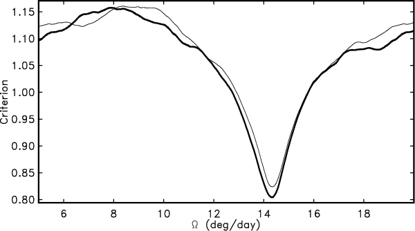
Figure 1:
Statistic
|
| Open with DEXTER | |
3.1 Mean angular velocity
For the first approximation we can assume that the mechanism generating the sunspots rotates as a rigid body. Then we can measure its angular velocity usingTo evaluate the significance of our results, we needed a proper method to calculate the error estimates. It is relatively easy to compute the errors of the polynomial fitting procedure. Depending on the degree of the fitted polynomial and hemisphere at hand, the typical standard errors are in the interval 0.001-0.002. Correspondingly we can state that for the particular data run the estimated mean rotation velocity for the Northern hemisphere is somewhat faster than the velocity for the Southern hemisphere.
To obtain a rough estimate of the sampling errors in our nonparametric context we used an approach which is known as a moving block bootstrap (Künsch 1989; Liu & Singh 1992; see also Lahiri 2003). In this method a large number (in our case 500) bootstrap samples are compiled from random sub-blocks of the original data sets. The block length is a defining parameter of the procedure. It must be long enough to take into account dependencies in the data and short enough to allow a proper reshuffling. The underlying theory of the method is developped for stationary sequences. Due to the cyclical nature of the solar activity we do not have a strictly stationary process and must therefore use general results with caution. This is why we calculated our error bars with three different block lengths: 10, 20 and 140. The first is a typical value, which is derived from the general theory, the second is chosen so that it is longer than the typical decorrelation time (see below), and the third one is essentially the mean length of the activity cycle.
Table 1: Results of the bootstrap claculations.
The results of the bootstrap calculations are presented in Table 1. Higher variance for short block length bootstrap runs can be explained by extra scatter, which results from inter-cycle sampling. For long blocks all phases of the cycle are equally well presented in every block. For shorter blocks the number of, say, sparsely populated blocks can be more fluctuating. This effect is smaller for the minima, which are computed using polynomial fitting.
It is evident from Table 1 that if we consider the data for the two hemispheres as two separate samples, it is not possible to reliably say which one rotates faster.
We also see from the table that the scatter of minima, which are calculated with polynomial fits, is significantly lower than scatter obtained for absolute minima. However, to be consistent with our nonparametric approach we will proceed below using absolute minima.
3.2 Differential rotation
Sunspots and other activity indicators rotate with different angular
velocities at different latitudes.
By tracking particular objects in
time it is possible to build a smooth curve to reveal the overall
pattern of this differential, latitude dependent, rotation. Our
statistic
![]() does not track single sunspots or the
actual movement of sunspot groups, as we include only the first
appearance of the sunspot groups.
This way we can check whether the spot-generating mechanism itself
rotates differentially or not. For that purpose we divided the observed
groups into four subsets along latitudes (per hemisphere) and computed
does not track single sunspots or the
actual movement of sunspot groups, as we include only the first
appearance of the sunspot groups.
This way we can check whether the spot-generating mechanism itself
rotates differentially or not. For that purpose we divided the observed
groups into four subsets along latitudes (per hemisphere) and computed
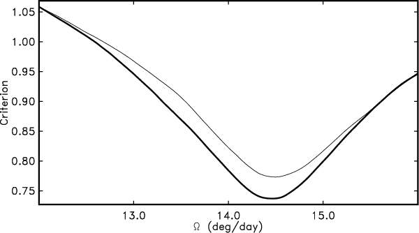
![]() for every group. The latitude limits for the subsets
where chosen to make them as equal in size as possible. The typical
curves are shown in Fig. 2. The exact determination of the
minima for the curves is somewhat complicated. If we locally fit
polynomials into the curves as we did above, we can get estimates with
high formal precision (0.001-0.002).
The differences between the absolute numerical minima and the
fitted minima, however, can be quite considerable (up to 0.045).
Error estimates from bootstrap calculations depend on the chosen block lengths and
are in the range of 0.04-0.12.
for every group. The latitude limits for the subsets
where chosen to make them as equal in size as possible. The typical
curves are shown in Fig. 2. The exact determination of the
minima for the curves is somewhat complicated. If we locally fit
polynomials into the curves as we did above, we can get estimates with
high formal precision (0.001-0.002).
The differences between the absolute numerical minima and the
fitted minima, however, can be quite considerable (up to 0.045).
Error estimates from bootstrap calculations depend on the chosen block lengths and
are in the range of 0.04-0.12.
|
Figure 2:
Statistic
|
| Open with DEXTER | |
Table 2: Differential rotation and break down times.
The full set of the absolute minima for all the eight curves is given in Table 2.
|
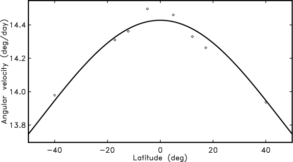
Figure 3: Differential rotation curve. |
| Open with DEXTER | |
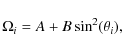
where
The results obtained in this section clearly demonstrate that the simple nonparametric method can be succesfully used to study the differential rotation of the solar activity tracers.
3.3 Break-down times
The results of the previous section clearly show that the longitudinally concentrated spot-generating mechanism is subject to differential rotation (to put this result into historical context see the review part in the paper by Usoskin et al. 2007). Kinematic mean-field dynamo theory predicts (e.g. Krause & Rädler 1980) that in the parameter regime where nonaxisymmetric dynamo modes can be excited, the nonaxisymmetric modes are non-oscillatory and rotate rigidly with angular velocity different from the overall rotation period. The phenomenon of phase-mixing, i.e. the nonaxisymmetric modes becoming affected by differential rotation, is against these predictions; our results, however, are consistent with the phase-mixing effect.Let us now try to quantify the effect of the differential rotation on
the nonaxisymmetric structures by calculating the characteristic time
needed to break down a longitudinally elongated stucture for different
latitude strips.
With the estimated B values from Eq. (10) we can define a break-down time for the strip
of latitudes
![]() in the number of rotations
in the number of rotations
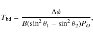
|
(11) |
where
3.4 Decorrelation time
So far we have demonstrated that the sunspot group distributions along
longitudes for sequential Carrington rotations are correlated.
We also computed the best fitting mean angular velocity ![]() for
several latitude strips, and as a result found out a clear
differential rotation pattern.
Next we were interested in estimating the approximate lifetimes of the
correlated features found from the sunspot data.
For that purpose we used the obtained mean angular velocities for
each latitude strip and computed
for
several latitude strips, and as a result found out a clear
differential rotation pattern.
Next we were interested in estimating the approximate lifetimes of the
correlated features found from the sunspot data.
For that purpose we used the obtained mean angular velocities for
each latitude strip and computed ![]() curves to learn how fast
the correlation between appropriately rotated longitude sets fades off.
curves to learn how fast
the correlation between appropriately rotated longitude sets fades off.
|
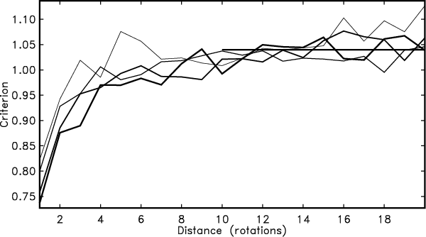
Figure 4:
Statistic |
| Open with DEXTER | |
|
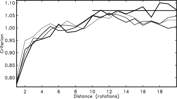
Figure 5:
Statistic |
| Open with DEXTER | |
The results of this analysis are displayed on
Figs. 4 and 5.
In these plots the thick horizontal lines indicate the asymptotic level of the
![]() curves (mean value of the
curves (mean value of the
![]() )
computed for the strips nearest to the equator.
As is evident from the plots, the inherent scatter
of the
)
computed for the strips nearest to the equator.
As is evident from the plots, the inherent scatter
of the ![]() curves is quite large; this is due to the physical
variability of the activity level and the roughness of the
statistic. Therefore it is hard to fix the point where the asymptotic
level is achieved. Some aspects of the curves, however, are quite
indicative.
First - the shortest decorrelation time is obtained for the
highest latitudes.
This is obvious because the width (in degrees) of the high altitude
strips is more extended and covers very differently rotating spot
groups. Secondly - the strips nearest to the equator show the longest
correlations. We can quite safely claim that a certain level of
correlation is visible up to a
time span of 10-15 rotations.
curves is quite large; this is due to the physical
variability of the activity level and the roughness of the
statistic. Therefore it is hard to fix the point where the asymptotic
level is achieved. Some aspects of the curves, however, are quite
indicative.
First - the shortest decorrelation time is obtained for the
highest latitudes.
This is obvious because the width (in degrees) of the high altitude
strips is more extended and covers very differently rotating spot
groups. Secondly - the strips nearest to the equator show the longest
correlations. We can quite safely claim that a certain level of
correlation is visible up to a
time span of 10-15 rotations.
Comparing the estimated decorrelation times for different latitude strips with the break-down times from Table 1 we can see that for lower latitudes the decorrelation times obtained from our analysis are much shorter than the estimated break-down times. For the highest latitude strip the decorrelation time is of the same order of magnitude than the break-down time. Part of this effect could be due to the enhanced diffusion of the field due to the stretching by the shear in angular velocity; the latitude dependence (shorter decorrelation times at high latitudes with the largest relative shear) would support this interpretation. It seems likely, however, that at least at lower latitudes stretching and enhanced turbulent diffusion acting on the magnetic field due to differential rotation are not the only effects at play.
4 Discussion
To put our results in a general context we will compare them with a sample of previous analyses.To a great extent the solar variability research is not based on a full set of sunspot observations, but on some aggregated form of data. Most typically the daily Wolf sunspot numbers are used. For instance Bogart (1982) analysed these numbers using autocorrelation functions and power spectra. The major results were quite similar to ours - the rotation period around 27 days was detected and the persistence of activity zones was claimed to be of the order of 10 solar rotations. In principle correlation functions and power spectra can be considered to be parameter-free statistics. The aggregated nature of the Wolf numbers, however, does not allow the analysis of the latitude dependence of active clusters.
There is a number of analyses that use longitudinal phase binning of the surface features. For instance in a series of papers Bai (1987, 1988) used comoving frames (as in our work) to seek rotation velocities, which enhance the statistical contrast of the longitudinal distribution of solar flares. The transformed longitudes for each trial rotation velocity were binned into 12 bins and the variance of obtained distributions was computed. The possibility of differential rotation was not taken into account. To study the persistence of particular active regions they were visually tracked and displayed as ``family trees''. In describing his results the author proposed a general scheme to characterize hierarchical patterns of solar activity:
- single events (sunpots, flares);
- active regions;
- activity complexes;
- active zones.
Probably the most popular method to study the kinematics of the solar surface features is a standard power spectrum analysis and its variants (just an example - Temmer et al. 2004; Giordano 2008). This kind of analysis can be applied to latitude strips and in this way the differential rotation can be taken into account. At a first glance the Fourier analysis seems to be essentially nonparametric. However, because it uses single harmonics as base functions, it prescribes a certain form of preferred activity distributions. The results of the Fourier method are often given as a list of certain periods, which show up in power spectra or on wavelet plots. The periodicity claim itself is quite a strong statement, as it is often very hard to find physically solid timing mechanisms for periods, which strongly differ from the obvious one - that of the solar rotation.
We wish to stress here that in the proposed statistical method no
assumptions about the particular form of the activity indicator
distributions are made. Even more - the statistics ![]() and
and ![]() are not seeking certain clusters or other kind of patterns, they
are just used to check whether the origins of surface
elements are correlated or not.
This makes the new method somewhat
similar to the method of ``family trees'' (Bai 2003) or
longitude-time diagrams (Brouwer & Zwaan 1990).
are not seeking certain clusters or other kind of patterns, they
are just used to check whether the origins of surface
elements are correlated or not.
This makes the new method somewhat
similar to the method of ``family trees'' (Bai 2003) or
longitude-time diagrams (Brouwer & Zwaan 1990).
The literature about the longitudinal distribution of solar activity indicators is so divers that it is not reasonable to compare our results with all of them. It suffices to state that the general patterns revealed so far are quite similar to those described above. The major shortcomings of the previously used methods include the dependence of the results on some prefixed parameters or on the choice of a particular distribution model.
5 Conclusions
When introducing a new method to analyse solar activity patterns we started from certain methodological principles:- Input data must be homogeneous, comprehensive and cover as long a time-base as possible.
- The analysis method must be free from any prefixed constants.
- The method must not depend on the model of the activity indicator distributions (unimodal, bimodal etc.).
- The computations must be as simple as possible.
- The distribution of sunspots is determined by the underlying large-scale mechanism that is more persistent than sunspots themselves. This shows up as a tendency of new sunspots to occur near the places where the previous sunspots were observed.
- The mean rotation velocity of the large-scale features for the
Northern hemisphere is
 deg/days and for the Southern
hemisphere
deg/days and for the Southern
hemisphere
 deg/days.
- The large-scale patterns of activity take part in differential rotation. The differential rotation curve is somewhat shallower if compared with curves obtained from sunspot tracking (see Zappalà & Zuccarello 1991).
- The strong tendency for the spot groups to cluster on a certain longitude peters out with time. The longest observable correlations can reach 10-15 Carrington rotations.
- The correlations between rotations are more pronounced for lower latitudes.
- The observation of the spot-generating mechanism being affected by differential rotation is suggestive of phase mixing occurring in the solar convection zone; such a phenomenon is not predicted by conventional mean-field dynamo theory.
We would like to thank the referee for useful suggestions. Part of this work was supported by the Estonian Science Foundation grant No. 6813 and Academy of Finland grant No. 112020. The authors thank the hospitality of NORDITA during the programme ``Solar and stellar dynamos and cycles''.
References
- Bai, T. 1987, ApJ, 314, 795 [NASA ADS] [CrossRef] [Google Scholar]
- Bai, T. 1988, ApJ, 328, 860 [NASA ADS] [CrossRef] [Google Scholar]
- Bai, T. 2003, ApJ, 585, 1114 [NASA ADS] [CrossRef] [Google Scholar]
- Beck, J. G. 1999, Sol. Phys., 191, 47 [NASA ADS] [CrossRef] [Google Scholar]
- Becker, U. 1955, Z. Astrophys., 37, 47 [Google Scholar]
- Bogart, R. S. 1982, Sol. Phys., 76, 155 [NASA ADS] [CrossRef] [Google Scholar]
- Brouwer, M. P., & Zwaan, C. 1990, Sol. Phys., 129, 221 [Google Scholar]
- Bumba, V., & Howard, R. 1965, ApJ, 141, 1502 [NASA ADS] [CrossRef] [Google Scholar]
- Castenmiller, M. J. M., Zwaan, C., & van der Zalm, E. B. J. 1986, Sol. Phys., 105, 237 [NASA ADS] [CrossRef] [Google Scholar]
- Gaizauskas, V., Harvey, K. L., Harvey, J. W., & Zwaan, C. 1983, ApJ. 265, 1056 [NASA ADS] [CrossRef] [Google Scholar]
- Giordano, S., & Mancuso, S. 2008, ApJ, 688, 656 [NASA ADS] [CrossRef] [Google Scholar]
- Juckett, D. 2003, A&A, 399, 731 [NASA ADS] [CrossRef] [EDP Sciences] [Google Scholar]
- Krause, F., & Rädler, K.-H. 1980, Mean-field magnetohydrodynamics and dynamo theory (Berlin: Akademie-Verlag) [Google Scholar]
- Künsch, H. R. 1989, The Annals of Statistics, 17, 1217 [Google Scholar]
- Lahiri, S. N. 2003, Resampling Methods for Dependent Data (New-York, Inc.: Springer-Verlag) [Google Scholar]
- Liu, R. Y., & Singh, K. 1992, in Exploring the Limits of the Bootstrap, ed. R. Lepage, & L. Billard (New York: Wiley), 225 [Google Scholar]
- Losh, N. M. 1938, Publ. Observ. Michigan, 7, 127 [Google Scholar]
- Mardia, K. V., & Jupp, P. 2000, Directional Statistics, 2nd edn. (John Wiley and Sons Ltd.) [Google Scholar]
- Pelt, J., Brooke, J., Korpi, M., & Tuominen, I. 2006, A&A, 460, 875 (PBKT) [NASA ADS] [CrossRef] [EDP Sciences] [Google Scholar]
- Pulkkinen, P., & Tuominen, I. 1998, A&A, 332, 748 [NASA ADS] [Google Scholar]
- Temmer, M., Veronig, A., Rybák, J., Brajsa, R., & Hanslmeier, A. 2004, Sol. Phys., 221, 325 [NASA ADS] [CrossRef] [Google Scholar]
- Trotter, D. E., & Billings, D. E. 1962, ApJ, 136, 1140 [NASA ADS] [CrossRef] [Google Scholar]
- Tuominen, I., & Virtanen, H. 1988, Adv. Space Res., 8, 141 [NASA ADS] [CrossRef] [PubMed] [Google Scholar]
- Usoskin, I. G., Berdyugina, S. V., & Poutanen, J. 2005, A&A, 441, 347 [NASA ADS] [CrossRef] [EDP Sciences] [Google Scholar]
- Usoskin, I. H., Berdyugina, S. V., Moss, D., & Sokoloff, D. D. 2007, Adv. Space Res., 40, 951 [NASA ADS] [CrossRef] [Google Scholar]
- Vitinskij, Ju. I. 1969, Sol. Phys., 7, 210 [NASA ADS] [CrossRef] [Google Scholar]
- Warwick, C. S. 1965, ApJ, 141, 500 [NASA ADS] [CrossRef] [Google Scholar]
- Zappalà, R. A., & Zuccarello, F. 1991, A&A, 242, 480 [NASA ADS] [Google Scholar]
Footnotes
All Tables
Table 1: Results of the bootstrap claculations.
Table 2: Differential rotation and break down times.
All Figures
|
|
Figure 1:
Statistic
|
| Open with DEXTER | |
| In the text | |
|
|
Figure 2:
Statistic
|
| Open with DEXTER | |
| In the text | |
|
|
Figure 3: Differential rotation curve. |
| Open with DEXTER | |
| In the text | |
|
|
Figure 4:
Statistic |
| Open with DEXTER | |
| In the text | |
|
|
Figure 5:
Statistic |
| Open with DEXTER | |
| In the text | |
Copyright ESO 2010
Current usage metrics show cumulative count of Article Views (full-text article views including HTML views, PDF and ePub downloads, according to the available data) and Abstracts Views on Vision4Press platform.
Data correspond to usage on the plateform after 2015. The current usage metrics is available 48-96 hours after online publication and is updated daily on week days.
Initial download of the metrics may take a while.