| Issue |
A&A
Volume 512, March-April 2010
|
|
|---|---|---|
| Article Number | A63 | |
| Number of page(s) | 15 | |
| Section | Extragalactic astronomy | |
| DOI | https://doi.org/10.1051/0004-6361/200913564 | |
| Published online | 02 April 2010 | |
Metal production in M 33: space and time
variations![[*]](/icons/foot_motif.png)
L. Magrini1 - L. Stanghellini2 - E. Corbelli1 - D. Galli1 - E. Villaver3
1 - INAF - Osservatorio Astrofisico di Arcetri, Largo E. Fermi 5, 50125
Firenze, Italy
2 - National Optical Astronomy Observatories, Tucson, AZ 85719, USA
3 - Universidad Autónoma de Madrid, Departamento de Física Teórica
C-XI, 28049 Madrid, Spain
Received 28 October 2009 / Accepted 18 December 2009
Abstract
Context. Nearby galaxies are ideal places to study
metallicity gradients in detail and their time evolution.
Aims. We analyse the spatial distribution of metals
in M 33 using a new sample and the literature data on
H II regions, and
constrain a model of galactic chemical evolution with H II region
and planetary nebula (PN) abundances.
Methods. We consider chemical abundances of a new
sample of H II regions
complemented with previous data sets. We compared H II region
and PN abundances obtained with a common set of observations
taken at MMT. With an updated theoretical model, we followed
the time evolution of the baryonic components and chemical abundances
in the disk of M 33, assuming that the galaxy is accreting gas
from an external reservoir.
Results. From the sample of H II regions,
we find that i) the 2D metallicity distribution has
an off-centre peak located in the southern arm; ii) the oxygen
abundance gradients in the northern and southern sectors,
as well as in the nearest and farthest sides,
are identical within the uncertainties, with slopes around
-0.03-4 dex kpc-1;
iii) bright giant H II regions
have a steeper abundance gradient than the other H II regions;
iv) H II regions
and PNe have O/H gradients very close within the errors;
v) our updated evolutionary model is able to reproduce the new
observational constraints, as well as the metallicity gradient
and its evolution.
Conclusions. Supported by a uniform sample of
nebular spectroscopic observations, we conclude that i) the
metallicity distribution in M 33 is very complex, showing a
central depression in metallicity probably due to observational bias;
ii) the metallicity gradient in the disk of M 33 has
a slope of -0.037 ![]() 0.009 dex kpc-1 in the whole
radial range up to
0.009 dex kpc-1 in the whole
radial range up to ![]() 8 kpc,
and -0.044
8 kpc,
and -0.044 ![]() 0.009 dex kpc-1 excluding the
central kpc; iii) there is little evolution in the
slope with time from the epoch of PN progenitor formation to
the present.
0.009 dex kpc-1 excluding the
central kpc; iii) there is little evolution in the
slope with time from the epoch of PN progenitor formation to
the present.
Key words: galaxies: abundances - galaxies: evolution - galaxies: individual: M 33
1 Introduction
Understanding the chemical evolution of nearby galaxies has become more
and more interesting in the recent past, given the wealth of new,
detailed data available for their stellar and gaseous components.
M 33 (NGC 598) is an ideal laboratory for testing
chemical evolution models. As a nearby blue star-forming
galaxy, with a large angular size (optical size 53![]()
![]() 83
83![]() ,
Holmberg 1958),
and an intermediate inclination (i = 53
,
Holmberg 1958),
and an intermediate inclination (i = 53![]() ),
it is one of the galaxies observed with the greatest
resolution and sensitivity. Distance estimates range from
730 kpc (Brunthaler et al. 2005) to
964 kpc (Bonanos et al. 2006).
In this paper we adopt an average value of 840 kpc
(Freedman et al. 1991).
Many spectroscopic studies are available, aiming at determining the
physical and chemical properties of its H II regions
(cf., e.g., Smith 1975;
Kwitter & Aller 1981;
Vílchez et al. 1988;
Willner & Nelson-Patel 2002;
Crockett et al. 2006;
Magrini et al. 2007a;
Rosolowsky & Simon 2008;
Rubin et al. 2008).
These H II regions trace
the present interstellar medium (ISM) and their metallicity is a
measure of the star formation rate (SFR) integrated over the whole
galaxy lifetime.
As a result, the metallicity of H II regions
gives interesting constraints to galactic chemical evolution models.
),
it is one of the galaxies observed with the greatest
resolution and sensitivity. Distance estimates range from
730 kpc (Brunthaler et al. 2005) to
964 kpc (Bonanos et al. 2006).
In this paper we adopt an average value of 840 kpc
(Freedman et al. 1991).
Many spectroscopic studies are available, aiming at determining the
physical and chemical properties of its H II regions
(cf., e.g., Smith 1975;
Kwitter & Aller 1981;
Vílchez et al. 1988;
Willner & Nelson-Patel 2002;
Crockett et al. 2006;
Magrini et al. 2007a;
Rosolowsky & Simon 2008;
Rubin et al. 2008).
These H II regions trace
the present interstellar medium (ISM) and their metallicity is a
measure of the star formation rate (SFR) integrated over the whole
galaxy lifetime.
As a result, the metallicity of H II regions
gives interesting constraints to galactic chemical evolution models.
In the past, studies of the metallicity gradient of
H II regions in
M 33 have shown a very steep profile. First quantitative
spectroscopic studies were carried out by Smith (1975), Kwitter
& Aller (1981)
and Vílchez et al. (1988).
Their observations, limited to the brightest and largest H II regions,
led to a radial oxygen gradient
about -0.1 dex kpc-1.
Considering the observations by the above researchers, Garnett
et al. (1997)
obtained an overall O/H gradient of -0.11 ![]() 0.02 dex kpc-1.
0.02 dex kpc-1.
With increasing sample sizes, flatter gradients have been
determined, in particular by i) Willner &
Nelson-Patel (2002)
who derive neon abundances of 25 H II regions
from infrared lines, obtaining a Ne/H gradient of
-0.034 ![]() 0.015 dex kpc-1;
ii) Crockett et al. (2006) who derive
even shallower gradients (-0.016
0.015 dex kpc-1;
ii) Crockett et al. (2006) who derive
even shallower gradients (-0.016 ![]() 0.017 dex kpc-1 for Ne/H and
-0.012
0.017 dex kpc-1 for Ne/H and
-0.012 ![]() 0.011 dex kpc-1
for O/H) from optical spectra of 6 H II regions;
iii) Magrini et al. (2007a) who
obtain an O/H gradient of 14 H II regions,
located in the radial range from
0.011 dex kpc-1
for O/H) from optical spectra of 6 H II regions;
iii) Magrini et al. (2007a) who
obtain an O/H gradient of 14 H II regions,
located in the radial range from ![]() 2 to
2 to ![]() 7.2 kpc with a slope
of -0.054
7.2 kpc with a slope
of -0.054 ![]() 0.011 dex kpc-1;
iv) Rosolowsky & Simon (2008) who observe the
largest sample of H II regions, 61,
finding a slope of -0.027
0.011 dex kpc-1;
iv) Rosolowsky & Simon (2008) who observe the
largest sample of H II regions, 61,
finding a slope of -0.027 ![]() 0.012 dex kpc-1 from
0.012 dex kpc-1 from ![]() 0.2 to
0.2 to
![]() 6 kpc;
v) Rubin et al. (2008)
who obtain Ne/H and S/H gradients from Spitzer infrared
spectra of -0.058
6 kpc;
v) Rubin et al. (2008)
who obtain Ne/H and S/H gradients from Spitzer infrared
spectra of -0.058 ![]() 0.014 dex kpc-1 and
-0.052
0.014 dex kpc-1 and
-0.052 ![]() 0.021 dex kpc-1, respectively.
0.021 dex kpc-1, respectively.
Rosolowsky & Simon (2008) attribute the large discrepancies in different authors' determinations to an intrinsic scatter of about 0.1 dex around the average gradient, but the scatter is unexplained by the abundance uncertainties. This kind of scatter is also seen in the Milky Way gradient from H II regions (e.g. Afflerbach et al. 1997), and it may be caused by metallicity fluctuations in the ISM and by the spiral arms. Thus a limited number of observations, coupled with a significant metallicity scatter at a given radius, may produce widely varying results. In the case of a shallow gradient this effect is even stronger; for example, for an abundance gradient of -0.02-0.03 dex kpc-1 in a galaxy with a radius of 10 kpc and a scatter of 0.1 dex, one would need more than 30 H II regions to obtain a good estimate of the slope of the gradient (Bresolin et al. 2009). Thus, only a large number of measurements can overcome the uncertainties engendered by the intrinsic variance and relatively shallow gradient of M 33.
Our sample is composed of 48 H II
regions. We derived the physical and chemical properties for
19 H II regions
which have not been observed previously, and for other
14 H II regions
whose chemical abundances have already been published. For the
remaining H II regions,
the faintness of their spectra did not allow any reliable
abundance determination, since their electron temperature (![]() )
could not be derived. We complemented these observations by a sample of
102 planetary nebulae (PNe), already presented by
Magrini et al. (2009a,
hereafter M09), observed during the same run. The main advantage of
observing a combined sample of H II regions
and PNe is being able to use not only the same observational set-up,
but also the same data reduction and analysis techniques, and to use
identical abundance determination methods.
)
could not be derived. We complemented these observations by a sample of
102 planetary nebulae (PNe), already presented by
Magrini et al. (2009a,
hereafter M09), observed during the same run. The main advantage of
observing a combined sample of H II regions
and PNe is being able to use not only the same observational set-up,
but also the same data reduction and analysis techniques, and to use
identical abundance determination methods.
Although our sample of H II regions does not add much to the literature, the presence of several objects in common with previous studies allows us to check the consistency of different sets of chemical abundance results. By including at the same time two stellar populations of different ages but with similar spectroscopic characteristics, our observations allowed us to study for the first time the global metallicity, its 2-dimensional (2D) distribution and its radial gradient, at two different epochs in the galaxy's lifetime avoiding biases introduced by different metallicity analysis. The aim of the present study is to settle the questions of the value of the metallicity gradient in M 33 and its time evolution. In this framework, the new observations of H II regions and PNe in M 33 complemented with the previous data represent the largest metallicity database available for an external galaxy.
In addition to metallicity data, recent results, such as the detection of inside-out growth in the disk of M 33 (Williams et al. 2009), the detailed analysis of the star formation both in the whole disk (Verley et al. 2009) and in several giant H II regions (Relano & Kennicutt 2009), stimulated us to revise the already existing chemical evolution model (M07b) and the star formation process in M 33. Particular attention was put on the observational constraints that our previous model failed to reproduce, such as the radial profile of the molecular gas and the relationship between the SFR and the molecular gas.
The paper is organized as follows. In Sect. 2 we describe our sample of H II regions observed with MMT. These data, together with a large literature dataset, allowed us to compute the metallicity gradient of H II regions again. In Sect. 3 we present the 2D distribution of the metallicity and the radial gradient of different types of H II regions. In Sect. 4 we discuss the off-centre metallicity peak and its origin. In Sect. 5 the data are compared with the prediction of chemical evolution model of M 33. Finally, our conclusions and a summary are given in Sect. 6.
2 The H II region dataset
Hot O-B stars ionize their surrounding medium, producing the
characteristic emission-line spectra of H II regions.
The H II regions of
M 33 studied in the literature span a wide range of
luminosities. Their intrinsic brightness led giant H II regions
to be preferred in the earlier studies (e.g. Kwitter &
Aller 1981;
Vilchez et al. 1988)
when only
relatively small telescopes were available. Smaller and fainter
H II regions have
instead been
the subject of later spectroscopic investigations (e.g., Magrini
et al. 2007a;
Rosolowsky & Simon 2008).
The latest abundance determinations have been restricted to the
H II regions with
available electron temperature measurements. Several emission-line
diagnostics of nebular ![]() are indeed present in the optical spectrum of an H II region,
namely: [O III] 4363 Å,
[N II] 5755 Å,
[S III] 6312 Å,
[O II] 7320-7330 Å.
Determining
are indeed present in the optical spectrum of an H II region,
namely: [O III] 4363 Å,
[N II] 5755 Å,
[S III] 6312 Å,
[O II] 7320-7330 Å.
Determining ![]() is the only way to derive the ionic and total chemical abundances
safely and accurately. An assumed
is the only way to derive the ionic and total chemical abundances
safely and accurately. An assumed ![]() could produce error of a factor of 2 or more in the final
chemical abundances (cf., e.g., Osterbrock & Ferland
1989). This is
why in the following analysis we include only those H II regions
whose
could produce error of a factor of 2 or more in the final
chemical abundances (cf., e.g., Osterbrock & Ferland
1989). This is
why in the following analysis we include only those H II regions
whose ![]() is directly measured.
is directly measured.
2.1 The MMT observations: data reduction and analysis
In November 2007, we obtained spectra of 48 H II regions
(and 102 PNe) in M 33 using the
MMT Hectospec fiber-fed spectrograph (Fabricant
et al. 2005).
The spectrograph was equipped with an atmospheric dispersion corrector
and it was used with a single setup: 270 mm-1
grating at a dispersion of 1.2 Å pixel-1.
The resulting total spectral coverage
ranged from approximately 3600 Å to 9100 Å, thus
including the basic emission-lines necessary
for determining their physical and chemical properties. The instrument
deploys 300 fibers
over a 1-degree diameter field of view, and the fiber diameter
is ![]() 1.5
1.5
![]() (6 pc adopting a distance
of 840 kpc to M 33).
(6 pc adopting a distance
of 840 kpc to M 33).
Some of the H II regions in our sample already have published spectra in the literature so we use them as control sample, while several are new. In Table 1 we list the H II regions from the total observed sample for which we can derive the physical and chemical properties. The identification names are from: BCLMP - Boulesteix et al. (1974); CPSDP - Courtes et al. (1987); GDK99 - Gordon et al. (1996); EPR2003 - Engargiola et al. (2003); MJ98 - Massey & Johnson (1998). The H II regions not identified in previous works are labled with LGC-HII-n as in Magrini et al. (2007a), standing for H II regions discovered by the Local Group Census project (cf. Corradi & Magrini 2006). The coordinates J2000.0 of the position of the fibers projected on the sky are shown in the third and forth columns. They do not correspond exactly to the centre of the emission line objects, but generally to the maximum [O III] emissivity.
Table 1: MMT observations of H II regions with chemical abundance determination.
The spectra were reduced using the Hectospec package. The
relative flux calibration was done observing the standard
star Hiltm600 (Massey et al. 1988) during the
nights of October 15 and November 27. The
emission-line fluxes were measured with the package SPLOT of IRAF![]() . Errors in the fluxes were
calculated taking the statistical error in the measurement of the
fluxes into account, as well as systematic errors of the flux
calibrations, background determination, and sky subtraction. The
observed line fluxes were corrected for the effect of the interstellar
extinction using the extinction law of Mathis (1990) with RV = 3.1.
We derived c(H
. Errors in the fluxes were
calculated taking the statistical error in the measurement of the
fluxes into account, as well as systematic errors of the flux
calibrations, background determination, and sky subtraction. The
observed line fluxes were corrected for the effect of the interstellar
extinction using the extinction law of Mathis (1990) with RV = 3.1.
We derived c(H![]() ), the logarithmic nebular
extinction, by using the weighted average of the
observed-to-theoretical Balmer ratios of H
), the logarithmic nebular
extinction, by using the weighted average of the
observed-to-theoretical Balmer ratios of H![]() ,
H
,
H![]() ,
and H
,
and H![]() to H
to H![]() (Osterbrock & Ferland 1989).
The detailed description of the data reduction and the plasma and
chemical analysis can be found in Magrini et al. (2009a,
hereafter M09). Spectra of two H II regions,
one close to the galactic centre and one in the outer part of the disk
are shown in Fig. 1.
(Osterbrock & Ferland 1989).
The detailed description of the data reduction and the plasma and
chemical analysis can be found in Magrini et al. (2009a,
hereafter M09). Spectra of two H II regions,
one close to the galactic centre and one in the outer part of the disk
are shown in Fig. 1.
![\begin{figure}
\par\vspace*{-1.5mm}\includegraphics[width=8.8cm,clip]{13564fg1.ps}
\vspace*{-1.5mm}\end{figure}](/articles/aa/full_html/2010/04/aa13564-09/img12.png)
|
Figure 1:
Two example spectra of H II
regions located at different galactocentric distance:
BCLMP 694 at |
| Open with DEXTER | |
Table 2
gives the results of our emission-line measurements and extinction
corrections for 33 H II regions
whose spectra were suitable for determining physical and chemical
properties.
The columns of Table 2
indicate: (1) H II region
name; (2) nebular extinction coefficient c(H![]() )
with its error; (3) emitting ion; (4) rest-frame
wavelength in Å; (5) measured line fluxes;
(6) absolute errors on the measured line fluxes;
(7) extinction corrected line fluxes. Both
)
with its error; (3) emitting ion; (4) rest-frame
wavelength in Å; (5) measured line fluxes;
(6) absolute errors on the measured line fluxes;
(7) extinction corrected line fluxes. Both
![]() (5) and
(5) and ![]() (7)
are expressed on a scale where H
(7)
are expressed on a scale where H![]() = 100.
Table 2
is published in its entirety at the CDS. A portion is shown
here for guidance regarding its form and content. The analysed
H II regions represent
about 2/3 of our sample. The remaining
1/3 H II regions
have noisy spectra and are distributed at all galactocentric radii. We
used the extinction-corrected intensities to obtain the electron
densities and temperatures. Electronic density was derived from the
intensities of the sulphur-line doublet [S II] 6716,
6731 Å.
We used the intensities of several emission-line ratios, when
available, to derive low and medium-excitation temperatures
(see also Osterbrock & Ferland 1989,
Sect. 5.2): [N II]
= 100.
Table 2
is published in its entirety at the CDS. A portion is shown
here for guidance regarding its form and content. The analysed
H II regions represent
about 2/3 of our sample. The remaining
1/3 H II regions
have noisy spectra and are distributed at all galactocentric radii. We
used the extinction-corrected intensities to obtain the electron
densities and temperatures. Electronic density was derived from the
intensities of the sulphur-line doublet [S II] 6716,
6731 Å.
We used the intensities of several emission-line ratios, when
available, to derive low and medium-excitation temperatures
(see also Osterbrock & Ferland 1989,
Sect. 5.2): [N II]![]() 5755/(
5755/(![]() 6548 +
6548 +
![]() 6584) and
[O II]
6584) and
[O II]![]() 3727/(
3727/(![]() 7320 +
7320 + ![]() 7330) for
low-excitation
7330) for
low-excitation ![]() ,
while [O III]
,
while [O III]![]() 4363/(
4363/(![]() 5007 +
5007 +
![]() 4959) and
[S III]
4959) and
[S III]![]() 6312/(
6312/(![]() 9069 +
9069 + ![]() 9532) for
medium-excitation
9532) for
medium-excitation ![]() .
We performed plasma diagnostics and ionic abundance calculation by
using the 5-level atom model included in the nebular
analysis package in IRAF/STSDAS (Shaw & Dufour 1994). The elemental
abundances are then determined by applying the ionization correction
factors (ICFs) following the prescriptions by Kingsburgh &
Barlow (1994) for
the case where only optical lines are
available. In the abundance analysis we adopted
.
We performed plasma diagnostics and ionic abundance calculation by
using the 5-level atom model included in the nebular
analysis package in IRAF/STSDAS (Shaw & Dufour 1994). The elemental
abundances are then determined by applying the ionization correction
factors (ICFs) following the prescriptions by Kingsburgh &
Barlow (1994) for
the case where only optical lines are
available. In the abundance analysis we adopted ![]() [N II]
and/or
[N II]
and/or ![]() [O II]
for computing the N+, O+,
S+ abundances, while
[O II]
for computing the N+, O+,
S+ abundances, while ![]() [O III]
and/or
[O III]
and/or ![]() [S III]
for O2+, S2+, Ar2+,
He+, and He2+. We
calculated the abundances of He I
and He II using the
equations of Benjamin et al. (1999) in two
density regimes, i.e.
[S III]
for O2+, S2+, Ar2+,
He+, and He2+. We
calculated the abundances of He I
and He II using the
equations of Benjamin et al. (1999) in two
density regimes, i.e. ![]() >
1000 cm-3 and
>
1000 cm-3 and ![]() 1000 cm-3. The
Clegg's collisional populations were taken into account (Clegg 1987). In
Table 3
we present the electron densities and temperatures, and the ionic and
total chemical abundances of our H II region
sample, which only includes H II regions
with at least one measured value of
1000 cm-3. The
Clegg's collisional populations were taken into account (Clegg 1987). In
Table 3
we present the electron densities and temperatures, and the ionic and
total chemical abundances of our H II region
sample, which only includes H II regions
with at least one measured value of ![]() .
The columns of Table 3
present: (1) identification name; (2) label of each
plasma diagnostic and abundances available; (3) relative
values obtained from our analysis. Table 3 is published in
its entirety at the CDS.
.
The columns of Table 3
present: (1) identification name; (2) label of each
plasma diagnostic and abundances available; (3) relative
values obtained from our analysis. Table 3 is published in
its entirety at the CDS.
Table 2: Observed and de-reddened fluxes (full table available at the CDS).
Table 3: Plasma diagnostics and abundances (full table available at the CDS).
We derived the temperature and density uncertainties using the
error propagation of the absolute
errors on the line fluxes. The errors on the ionic and total abundances
were computed taking
the uncertainties in the observed fluxes, in the electron temperatures
and densities, and in c(H![]() )
into account. In Table 4 a summary of
the total abundances He/H, O/H, N/H, Ne/H, S/H
and Ar/H and their errors are presented. The
He abundance is shown by number with its absolute error, while
the metal abundances are expressed in the form of
)
into account. In Table 4 a summary of
the total abundances He/H, O/H, N/H, Ne/H, S/H
and Ar/H and their errors are presented. The
He abundance is shown by number with its absolute error, while
the metal abundances are expressed in the form of ![]() with errors expressed in dex. The last row indicates the
average abundances computed by number.
with errors expressed in dex. The last row indicates the
average abundances computed by number.
2.2 The PN data-set
The PN population of M 33 was studied by Magrini
et al. (2009a)
using multi-fiber
spectroscopy with Hectospec at the MMT with the same spectroscopic
setup and during the same nights
as the H II region
observations presented here. Spectra of 102 PNe were analysed
and plasma diagnostics and chemical abundances obtained for
93 PNe where the necessary diagnostic lines were measured. The
data reduction and the plasma diagnostics followed exactly the same
procedure as described in the present paper, thus ensuring that no
biases are introduced for the different analysis of the spectra.
About 20![]() of the studied PNe have young progenitors, the so-called
type I PNe. The rest of the PNe in the sample are the
progenies of an old disk stellar population, with main sequence masses M <
3
of the studied PNe have young progenitors, the so-called
type I PNe. The rest of the PNe in the sample are the
progenies of an old disk stellar population, with main sequence masses M <
3 ![]() and ages t > 0.3 Gyr.
A tight relation between the O/H and Ne/H abundances
was found, excluding that both elements have been altered by
PN progenitors and supporting the validity of oxygen as a good
tracer of the ISM composition at the epoch of the
progenitors' birth.
and ages t > 0.3 Gyr.
A tight relation between the O/H and Ne/H abundances
was found, excluding that both elements have been altered by
PN progenitors and supporting the validity of oxygen as a good
tracer of the ISM composition at the epoch of the
progenitors' birth.
Table 4: The chemical abundances of our MMT sample.
3 The metallicity distribution in M 33
The large amount of chemical abundance data from H II regions
in M 33 allow us to analyse the spatially-resolved
distribution of metals in the ISM. In this section, we present
the radial distribution and the map of O/H, using the new data
presented in this paper and all previous oxygen determinations for
which ![]() has been measured.
has been measured.
3.1 The metallicity gradient of H II regions
Our cumulative sample includes: i) H II regions
by Magrini et al. (2007a),
which includes abundances from their own sample and previous abundance
determinations (all with ![]() and with abundances recomputed uniformly); ii) the sample by
Rosolowsky & Simon (2008);
iii) the present sample (see Table 3).
In Fig. 2,
we show the oxygen abundance as a function of galactocentric distance
for the cumulative sample of H II regions.
In this figure each point corresponds to a single region;
i.e., we do not plot multiple measurements for the same region
but only the value with the lowest error. Note the large dispersion in
the radial region between 1 and 2 kpc from the centre
caused by several high- and low-metallicity regions, located in the
southern arm (see Sect. 3.3), which might be related
to the presence of a bar (e.g., Corbelli & Walterbos 2007). We
applied the routine fitexy in Numerical Recipes
(Press et al. 1992)
to fit the relation between the oxygen abundances and the
galactocentric distances, taking their errors into account and
minimizing
and with abundances recomputed uniformly); ii) the sample by
Rosolowsky & Simon (2008);
iii) the present sample (see Table 3).
In Fig. 2,
we show the oxygen abundance as a function of galactocentric distance
for the cumulative sample of H II regions.
In this figure each point corresponds to a single region;
i.e., we do not plot multiple measurements for the same region
but only the value with the lowest error. Note the large dispersion in
the radial region between 1 and 2 kpc from the centre
caused by several high- and low-metallicity regions, located in the
southern arm (see Sect. 3.3), which might be related
to the presence of a bar (e.g., Corbelli & Walterbos 2007). We
applied the routine fitexy in Numerical Recipes
(Press et al. 1992)
to fit the relation between the oxygen abundances and the
galactocentric distances, taking their errors into account and
minimizing ![]() .
Typical errors on the de-projected galactocentric distances associated
with the uncertainty on the inclination were less than 0.1 kpc
(Magrini et al. 2007a).
The fit to the complete sample gives a gradient of
.
Typical errors on the de-projected galactocentric distances associated
with the uncertainty on the inclination were less than 0.1 kpc
(Magrini et al. 2007a).
The fit to the complete sample gives a gradient of
where
which is consistent within the errors with the gradient from the larger sample. In the rest of the paper, we use the larger and more complete sample when discussing the metallicity gradient and its possible time variation, but excluding the first kpc region where only a few low metallicity regions were analysed. We discuss the possible reasons for the lower value of the central metallicity later in this section and in Sect. 4. The O/H gradient of the whole sample of H II regions sample, excluding the central 1 kpc, is
We also checked the metallicity gradient by tracing it in different areas of the galaxy, namely in the northwest and in the southeast halves, separately, and in the nearest and in the farthest sides. The results are shown in Fig. 3. The northern and southern gradients, as well as those relative to the nearest and farthest sides, are identical within the uncertainties, with slopes around -0.03-4 dex kpc-1. The only difference found between the metallicity gradients obtained for sections of the galaxy is the presence of a high metallicity peak in the southern arm. In conclusion, the present H II region sample (literature + present-work, 103 objects), including only nebulae with measured
Stellar abundances were obtained by Herrero et al. (1994) for
AB-supergiants, McCarthy et al. (1995) and Venn
et al. (1998)
for A-type supergiant stars, and Monteverde et al. (1997, 2000) and
Urbaneja et al. (2005)
for B-type supergiant stars. The largest sample of Urbaneja
et al. (2005)
gave a O/H gradient of -0.06 ![]() 0.02 dex kpc-1. Recently, U
et al. (2009)
has presented spectroscopic observations of a set of A and
B supergiants. They determined stellar metallicities and
derived the metallicity gradient in the disk of M 33, finding
solar metallicity at the centre and 0.3 solar in the outskirts
at a distance of 8 kpc. Their average metallicity gradient is
-0.07
0.02 dex kpc-1. Recently, U
et al. (2009)
has presented spectroscopic observations of a set of A and
B supergiants. They determined stellar metallicities and
derived the metallicity gradient in the disk of M 33, finding
solar metallicity at the centre and 0.3 solar in the outskirts
at a distance of 8 kpc. Their average metallicity gradient is
-0.07 ![]() 0.01 dex kpc-1. At a
given radius, H II regions
have abundances slightly below the stellar results, and this is
probably due to the depletion of oxygen in H II regions
on dust grains (e.g., Bresolin et al. 2009). The
slopes of the two gradients agree if the comparison is done between
about 1 ant 8 kpc. The cause of the difference
between the supergiant and H II region
gradient is the metallicity value in the central regions.
In fact, the H II regions
located within 1 kpc from centre have metallicity below solar, whereas
the supergiants are metal rich, ranging from solar values to above
solar. The origin of this discrepancy is not the temperature gradients
within the nebulae (Stasinska 2005)
because they become important at higher metal abundances.
0.01 dex kpc-1. At a
given radius, H II regions
have abundances slightly below the stellar results, and this is
probably due to the depletion of oxygen in H II regions
on dust grains (e.g., Bresolin et al. 2009). The
slopes of the two gradients agree if the comparison is done between
about 1 ant 8 kpc. The cause of the difference
between the supergiant and H II region
gradient is the metallicity value in the central regions.
In fact, the H II regions
located within 1 kpc from centre have metallicity below solar, whereas
the supergiants are metal rich, ranging from solar values to above
solar. The origin of this discrepancy is not the temperature gradients
within the nebulae (Stasinska 2005)
because they become important at higher metal abundances.
![\begin{figure}
\par\includegraphics[angle=-90,width=8cm,clip]{13564fg2.ps}
\end{figure}](/articles/aa/full_html/2010/04/aa13564-09/img27.png)
|
Figure 2: The O/H radial gradient for the cumulative H II region sample: filled circles are the MMT observations (new and control samples), empty circles are the literature abundances. The continuous line is the weighted linear least-square fit of Eq. (3), i.e., with a radial range from 1 to 8 kpc from the M 33 centre. The dashed vertical line indicates the regions located at its left-side and excluded from the fit. |
| Open with DEXTER | |
Recent observations of 25 H II
regions by Rubin et al. (2008)
with Spitzer have allowed a measurement of the Ne/H
and S/H gradient across the disk of M 33 showing no
decrease in chemical abundances in the central regions.
Infrared Ne and S emission lines do not have a strong
dependence on ![]() ,
and consequently their abundances can be determined even without a
temperature measurement.
,
and consequently their abundances can be determined even without a
temperature measurement.
One way to explain the low metallicity in the central
1.0 ![]() 1.0 kpc2 area is related to
the criterion used for H II regions.
Usually, chemical abundances derived from optical spectroscopy rely on
direct measurement of the electron temperature, given by the
[O III] 4363 Å
emission line. This emission line is inversely proportional to the
oxygen abundance and barely detectable for
O/H > 8.6 from an average luminosity nebula
(e.g., Nagao et al. 2006). The request
for [O III] 4363 Å
detection might determine a bias towards lower metallicity, with the
exclusion of the highest metallicity nebulae. This could explain the
differences between the optical spectroscopy results and both the
stellar abundance determinations, and the H II region
infrared spectroscopy.
1.0 kpc2 area is related to
the criterion used for H II regions.
Usually, chemical abundances derived from optical spectroscopy rely on
direct measurement of the electron temperature, given by the
[O III] 4363 Å
emission line. This emission line is inversely proportional to the
oxygen abundance and barely detectable for
O/H > 8.6 from an average luminosity nebula
(e.g., Nagao et al. 2006). The request
for [O III] 4363 Å
detection might determine a bias towards lower metallicity, with the
exclusion of the highest metallicity nebulae. This could explain the
differences between the optical spectroscopy results and both the
stellar abundance determinations, and the H II region
infrared spectroscopy.
![\begin{figure}
\par\includegraphics[angle=-90,width=8cm,clip]{13564fg3.ps}\vspace*{5mm}
\includegraphics[angle=-90,width=8cm,clip]{13564fg4.ps}
\end{figure}](/articles/aa/full_html/2010/04/aa13564-09/img28.png)
|
Figure 3: The O/H radial gradient obtained in different regions of M 33. Top: nearest side (filled squares) and farthest side (empty squares) gradient. Bottom: North (filled squares) and South (empty squares) gradient. In each panel the weighted linear least-square fits of the two regions are shown with two lines (continuous and dotted). |
| Open with DEXTER | |
3.2 The abundance gradients of the other chemical elements
Our analysis allowed us to measure other chemical elements in addition to oxygen, as He/H, N/H, Ne/H, S/H and Ar/H. The more reliable measurement is that of oxygen for the reasons illustrated in the Appendix, and we use it to follow the chemical evolution of M 33. Nevertheless the other chemical elements are measured in enough H II regions to compute their radial gradients.
In Table 5
we show the slopes and central abundance values of the radial gradients
of N/H, Ne/H, S/H and Ar/H of our sample of H II regions.
We did not calculate the radial gradient of He/H because we measured
only the ionized fraction of He in H II regions,
which is only a small part of the total helium abundance. All gradients
have a negative slope, consistent, within the errors, with the slope
found for O/H, while N/H is a bit steeper, as already noticed, e.g., by
Magrini et al. (2007a).
Its different behaviour with respect to the ![]() -elements,
as oxygen, neon, sulphur, and argon, comes from the different
places of production.
-elements,
as oxygen, neon, sulphur, and argon, comes from the different
places of production. ![]() -elements
are indeed produced by SNe II, which are the final phase of
the evolution of massive stars, while nitrogen is one of the final
products of the evolution of long-lived low- and intermediate-mass
stars. This is discussed in detail in Sect. 5. Finally,
there is a very good agreement of the S/H and Ne/H gradients
with those derived from the infrared spectra of H II regions
by Rubin et al. (2008),
for which they found a gradient of -0.058
-elements
are indeed produced by SNe II, which are the final phase of
the evolution of massive stars, while nitrogen is one of the final
products of the evolution of long-lived low- and intermediate-mass
stars. This is discussed in detail in Sect. 5. Finally,
there is a very good agreement of the S/H and Ne/H gradients
with those derived from the infrared spectra of H II regions
by Rubin et al. (2008),
for which they found a gradient of -0.058 ![]() 0.014 dex kpc-1
for Ne/H and -0.052
0.014 dex kpc-1
for Ne/H and -0.052 ![]() 0.021 dex kpc-1
for S/H.
0.021 dex kpc-1
for S/H.
Table 5: The radial gradients of N/H, Ne/H, S/H and Ar/H.
3.3 The population-dependent metallicity gradient: giant vs. faint and compact H II regions
We now examine whether any selection effect can be responsible for the
difference between the steep gradient found in the early studies and
the shallower gradient of this work. To this goal, we
subdivided the sample of H II regions
according to their projected size and surface brightness in the H![]() emission-line.
Then, we computed the intrinsic luminosity and the radius in an
H
emission-line.
Then, we computed the intrinsic luminosity and the radius in an
H![]() emission-line
calibrated map (courtesy of Walterbos) for each nebula of the whole
sample.
Defining the surface brightness (SB) as the ratio between the total
flux and the area expressed in arcsec2,
we subdivided the sample according to their size and SB.
Considering their size, we defined them as small if
their radius R < 15
emission-line
calibrated map (courtesy of Walterbos) for each nebula of the whole
sample.
Defining the surface brightness (SB) as the ratio between the total
flux and the area expressed in arcsec2,
we subdivided the sample according to their size and SB.
Considering their size, we defined them as small if
their radius R < 15
![]() (60 pc at the distance 840 kpc) and as large
if R
(60 pc at the distance 840 kpc) and as large
if R ![]() 15
15
![]() .
Considering their surface brightness, we define them as bright
if their surface brightness SB > 5.5
.
Considering their surface brightness, we define them as bright
if their surface brightness SB > 5.5 ![]() 10-19 erg cm-2 s-1 arcsec-1,
and as faint if SB is lower than this limit. The
four combinations are allowed, i.e. H II regions
can be small and either bright
or faint, or large and
again bright or faint. In
Table 6
we show the galactocentric distance,
10-19 erg cm-2 s-1 arcsec-1,
and as faint if SB is lower than this limit. The
four combinations are allowed, i.e. H II regions
can be small and either bright
or faint, or large and
again bright or faint. In
Table 6
we show the galactocentric distance,
![]() ,
the H
,
the H![]() observed
total flux,
observed
total flux,
![]() ,
the radius, R, and the SB, of the
so-called giant regions, i.e. those with
SB > 5.5
,
the radius, R, and the SB, of the
so-called giant regions, i.e. those with
SB > 5.5 ![]() 10-19 erg cm-2 s-1 arcsec-1
and R
10-19 erg cm-2 s-1 arcsec-1
and R ![]() 15
15
![]() .
.
To compare the total population with the giant
H II regions, we show in
Fig. 4
the oxygen abundances of the cumulative sample, averaged in bins of
1 kpc each, together with the abundances of each single giant
H II region. The
O/H gradient of the H II regions
in Table 6,
computed with a weighted linear least-square fit, is
The gradient of the remaining sample is the same of given in Eq. (1). The giant regions show a significantly steeper gradient, consistent with the gradients by Smith (1975), Kwitter & Aller (1981), Vílchez et al. (1988), and Garnett et al. (1997). The question is whether this gradient is really significantly different from the whole sample, and if this is the case, what is the reason of such different behaviour.
Owing to the small number of giant
H II regions
(9 in total), the uncertainty on the slope
of their gradient is high. Thus it could still be in partial agreement,
within the errors, with the larger sample, and their difference might
stem from metallicity fluctuations in the ISM. On the other hand, the
characteristics of the giant regions might be truly
different from the average sample. For example large self-bound units
are not destroyed by massive stars and thus retain their original
structure and get continuously enriched by SF. However, while
this might be the case for the metallicity peak near the centre, it
does predict that giant regions should have higher metallicity at all
galactocentric radii, which is clearly not the case. Moreover,
in a recent paper, Relaño & Kennicutt (2009) studied the
star formation in luminous H II regions
in M 33, which correspond mostly to our giant
H II regions. They found
that the observed UV and H![]() luminosities
are consistent with a young stellar population (3-4 Myr), born
in an instantaneous burst. Thus the steeper gradient might result form
a combination of a small statistics and of a metal self-enrichment
effect in the giant region sample.
luminosities
are consistent with a young stellar population (3-4 Myr), born
in an instantaneous burst. Thus the steeper gradient might result form
a combination of a small statistics and of a metal self-enrichment
effect in the giant region sample.
Table 6: Giant H II regions with derived chemical abundances.
![\begin{figure}
\par\includegraphics[angle=-90,width=8cm]{13564fg5.ps}
\end{figure}](/articles/aa/full_html/2010/04/aa13564-09/img32.png)
|
Figure 4: The O/H radial gradient: the giant H II regions (empty triangles) and the complete sample averaged in bins, each 1 kpc wide (filled squares). The continuous line is the weighted mean least square fit of the giant H II region sample, while the dotted line refers to the complete sample. |
| Open with DEXTER | |
3.4 The 2-dimensional distribution of metals
The usual way to study the metallicity distribution in disk galaxies is
to average it azimuthally, assuming that i) the centre of the
galaxy coincides with the peak of the metallicity distribution and
ii) the metallicity distribution is axially symmetric. The
large number of metallicity measurements in M 33, both from
H II regions and from
PNe, allowed us to reconstruct not only
their radial gradient, but also their spatial distribution projected
onto the disk. In Fig. 5, we show the
two-dimensional metallicity distributions for M 33 from
H II regions and from
PNe superimposed to a contour map of the stellar mass distribution
derived from the JHK image, a composition of the image of
Regan & Vogel (1994)
and the 2MASS image. The O/H abundances were averaged
in bins of 0.8 ![]() 0.8 kpc2. The white pixels indicate
areas where metallicity measurements are lacking: for H II regions
they generally correspond to the interarm regions, while for PNe to
spiral arms.
0.8 kpc2. The white pixels indicate
areas where metallicity measurements are lacking: for H II regions
they generally correspond to the interarm regions, while for PNe to
spiral arms.
![\begin{figure}
\par\includegraphics[angle=90,width=8cm,clip]{13564fg6.ps}\vspace*{5mm}
\includegraphics[angle=90,width=8cm,clip]{13564fg7.ps}
\end{figure}](/articles/aa/full_html/2010/04/aa13564-09/img33.png)
|
Figure 5:
The oxygen abundance maps of M 33 (60 |
| Open with DEXTER | |
The H II regions with the highest metallicity are not located in the optical centre of the galaxy (0, 0 in the map), but rather lie at radius 1-2 kpc in the southeast direction. Also in the case of PNe, most of the metal rich PNe are located in the southern part of M 33, from 2 to 4 kpc from the centre. However the lack of known PNe in the northern spiral arm at the same distance of the southern metal-rich PNe (because of the extended H II regions not allowing the identification of stellar emission-line sources) does not allow a complete 2D picture of their metal distribution around the central regions.
To estimate the location of the off-centre metallicity peak
for the H II region map,
we divided its squared 10![]()
![]() 10
10![]() region,
centered at RA 1:33:50.9 dec 30:39:36
(M 33 centre from the 2MASS survey,
Skrutskie et al. 2006),
with a 10
region,
centered at RA 1:33:50.9 dec 30:39:36
(M 33 centre from the 2MASS survey,
Skrutskie et al. 2006),
with a 10 ![]() 10 grid. We computed the radial O/H gradients varying
the central position in the grid and then finding the one that
minimizes the scatter of the gradient. We found an off-centre position
at RA 1:33:59 dec 30:33:35 (J2000.0), which
corresponds to the location of the high-metallicity H II regions
in the southern arm. The oxygen gradient measured from this central
position of the whole H II region
population, including also the central objects, is
10 grid. We computed the radial O/H gradients varying
the central position in the grid and then finding the one that
minimizes the scatter of the gradient. We found an off-centre position
at RA 1:33:59 dec 30:33:35 (J2000.0), which
corresponds to the location of the high-metallicity H II regions
in the southern arm. The oxygen gradient measured from this central
position of the whole H II region
population, including also the central objects, is
and it is shown in Fig. 6. The gradient of Eq. (5) is flatter and with a somewhat lower absolute dispersion than the one in Eq. (1). The reduction of the dispersion in the O/H gradient due to the displacement of the galaxy centre is not enough strong to confirm that the metallicity maximum corresponds to the real centre of the metallicity distribution.
![\begin{figure}
\par\includegraphics[angle=-90,width=8cm,clip]{13564fg8.ps}
\end{figure}](/articles/aa/full_html/2010/04/aa13564-09/img35.png)
|
Figure 6: The O/H radial gradient computed with the centre located at RA 1:33:59 dec 30:33:35 (J2000.0) to minimize the dispersion in the slope of the radial gradient. |
| Open with DEXTER | |
4 Why is the metallicity peak off-centre?
In the following, we examine several possibilities to explain the presence of the off-centre metallicity maximum and the low metallicity measured in the central region: i) a local effect of ISM metallicity fluctuations; ii) the lack of dominant gravitational centre in the galaxy; iii) the selection criterion of H II regions for metallicity determination.
4.1 Local metallicity fluctuations
Simon & Rosolowsky (2008) have already noticed the non-axisymmetric distribution of H II region abundances and suggest that the material enriched by the most recent generation of star formation in the arm might not have been azimuthally mixed through the galaxy. A strong OB association located in the southern arm might be responsible for the enhancement enrichment at the location of the metallicity peak. Velocity shear is present in M 33 even at small radii because of the slow rise in the rotation curve (Corbelli 2003). At the peak location, differential rotation will shear up the bubble of metals produced in the surrounding ISM in about 108 yrs. The timescale seems long enough to allow vigorous star formation at a particular location to enrich the ISM of metals well above the average value. However, the large dispersion in the metallicity around the peak location seems to rule out an inefficient azimuthal mixing or redistribution of the metals.
4.2 The lack of a gravitational centre
The non-axysymmetric metallicity distribution might be related to a
general non-axisymmetric character of central regions of M 33,
noticed in the past by several authors. Colin & Athanassoula (1981) found that
the young population displacement is located towards the southern side
of M 33 and amounts to approximately 2-3![]() ,
i.e. 480-720 kpc. Using evidence of other asymmetries
in the inner regions of M 33, such as those present in the
distribution of H I atomic
gas, of H II regions,
and in the kinematics, they proposed a bulge centre presently located
in the northern part of the galaxy, which is rotating retrogradely
around the barycenter of the galaxy.
The analysis of infrared images (Minniti et al. 1993), however,
seems to point out to a small bulge with a much smaller displacement
the one advocated by Colin & Athanassoula (1981).
A detailed analysis of the kinematics of the innermost regions
of M 33 by Corbelli & Walterbos (2007) confirms
asymmetries in the stellar and gas velocities, which however seem more
related to the presence of a weak bar. The exact galaxy centre is
uncertain on scales of a few arcsec. Thus, even if
M 33 lacks of a dominant gravitational centre of M 33
and the bright central cluster might migrate around it,
it seems unlikely that the centre of the galaxy is off by
several hundreds pc from where the bright cluster lie. The
marginal gain in the dispersion in re-computing the metallicity
gradient from an off-centre position (see previous section)
confirms that this hypothesis seems unlikely.
,
i.e. 480-720 kpc. Using evidence of other asymmetries
in the inner regions of M 33, such as those present in the
distribution of H I atomic
gas, of H II regions,
and in the kinematics, they proposed a bulge centre presently located
in the northern part of the galaxy, which is rotating retrogradely
around the barycenter of the galaxy.
The analysis of infrared images (Minniti et al. 1993), however,
seems to point out to a small bulge with a much smaller displacement
the one advocated by Colin & Athanassoula (1981).
A detailed analysis of the kinematics of the innermost regions
of M 33 by Corbelli & Walterbos (2007) confirms
asymmetries in the stellar and gas velocities, which however seem more
related to the presence of a weak bar. The exact galaxy centre is
uncertain on scales of a few arcsec. Thus, even if
M 33 lacks of a dominant gravitational centre of M 33
and the bright central cluster might migrate around it,
it seems unlikely that the centre of the galaxy is off by
several hundreds pc from where the bright cluster lie. The
marginal gain in the dispersion in re-computing the metallicity
gradient from an off-centre position (see previous section)
confirms that this hypothesis seems unlikely.
4.3 Selection criterion
That the average metallicity at the centre seems lower than at 1.5 kpc is hard to explain in the framework of an inside-out disk formation scenario. We now discuss the possibility than in the central regions the metallicity might be higher than reported in this paper because of a bias in the H II region selection. As explained in Sect. 3.1 the inclusion of H II regions in our sample requires determining of the electron temperature through the detection of the faint oxygen auroral line. As the metallicity increases the line becomes so faint as to be detectable only in bright complexes. The centre of M 33 lacks of vigorous star-forming sites, so the most cooler, metal rich H II regions have the oxygen auroral line below the detection threshold. To prove that this might be the case we searched the literature for the existing H II region spectra inside 1.5 kpc radius, which were not included in our database because of the undetectable [O III] 4363 line. We found 4 H II regions in the database of Magrini et al. (2007a) for which optical spectroscopy is available but no detection of temperature diagnostic lines. Their names, coordinates, galactocentric distances, assumed electron temperatures, and oxygen abundances from M07a fluxes are shown in Table 7.
Table 7:
H II regions in the central
regions without direct ![]() measurement.
measurement.
In Fig. 7
we plot the relationship between the electron temperature and the
galactocentric distance for the complete H II region
sample. The weighted mean least square fit gives a relationship between
the two quantities
where
![\begin{figure}
\par\includegraphics[angle=-90,width=8cm,clip]{13564fg9.ps}
\end{figure}](/articles/aa/full_html/2010/04/aa13564-09/img37.png)
|
Figure 7:
The radial gradient of |
| Open with DEXTER | |
![\begin{figure}
\par\includegraphics[angle=-90,width=8cm,clip]{13564fg10.ps}
\end{figure}](/articles/aa/full_html/2010/04/aa13564-09/img38.png)
|
Figure 8:
The O/H radial gradient: the symbols for the H II regions
with a positive detection of |
| Open with DEXTER | |
Using the intensities by M07a, complemented with upper limit measurements of the [O II] 7320-7330 Å when not available in the original paper, we roughly estimated the oxygen abundance of the four H II regions located within 1.5 kpc. Their location in the radial gradient is shown in Fig. 8. The sources clearly lie above the average metallicity determined in the centre of our database. It is therefore likely that the adopted criterion for source selection, based on the positive detection of lines for determining the electron temperature, might be responsible for the low metallicity derived in the centre.
In the 1.5 kpc central region, there are
8 H II regions
with measured electron temperature having oxygen abundances from ![]() 8 to
8 to ![]() 8.5
(see Fig. 1),
namely B0043b (O/H 8.214), B0029 (8.211),
B0038b (8.391), B0016 (7.98),
B0079c (8.386), B0027b (8.37),
B0033b (8.399), B0090 (8.506). Their metal abundance
and dispersion are consistent with the hypothesis that we are missing
several high-metallicity regions within 1.5 kpc of the centre
since they only seem to trace the low metallicity side of the
distribution present at each given radius. Similarly, this bias
partially explains the different gradient of the giant
H II regions: we only
include metal-rich H II regions
(with metallicity above a critical value) in the sample if
they are very luminous because only these show detectable temperature
diagnostic lines.
8.5
(see Fig. 1),
namely B0043b (O/H 8.214), B0029 (8.211),
B0038b (8.391), B0016 (7.98),
B0079c (8.386), B0027b (8.37),
B0033b (8.399), B0090 (8.506). Their metal abundance
and dispersion are consistent with the hypothesis that we are missing
several high-metallicity regions within 1.5 kpc of the centre
since they only seem to trace the low metallicity side of the
distribution present at each given radius. Similarly, this bias
partially explains the different gradient of the giant
H II regions: we only
include metal-rich H II regions
(with metallicity above a critical value) in the sample if
they are very luminous because only these show detectable temperature
diagnostic lines.
5 The chemical evolution of M 33
The metallicity gradient derived in Sect. 3.1 from our sample of H II regions characterizes the ISM composition in M 33 at the present time. Together with the metallicity gradient from the PN population (M09), these data allow setting new constraints on current models of galactic chemical evolution.
The model of M07b, specifically designed for M 33, is able to predict the radial distribution of molecular gas, atomic gas, stars, SFR, and the time evolution of the metallicity gradient. In the following, we discuss the modifications needed to reproduce the metallicity gradient of H II regions and PNe derived in this work and in M09.
5.1 A revised model of chemical evolution
The multiphase model adopted by M07b follows the formation and
destruction of diffuse gas, clouds, and stars, by means of the simple
parameterizations of physical processes (e.g. Ferrini
et al.
1992).
In particular, the SFR is the result of two processes:
cloud-cloud interactions (the dominant process) and star
formation induced by the interaction of massive stars on molecular
clouds. At variance with other models, the relationship
between the SFR surface density,
![]() ,
and the molecular gas surface density,
,
and the molecular gas surface density,
![]() (the so-called Schmidt law) is thus a by-product of
the model and is not assumed. In general, the relation between
the surface density of total gas and SFR has a slope of 1.4
(the so-called Schmidt law) is thus a by-product of
the model and is not assumed. In general, the relation between
the surface density of total gas and SFR has a slope of 1.4 ![]() 0.1,
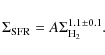
but the slope can vary from galaxy to galaxy (Kennicutt 1998a).
In the particular case of M 33, a tight
correlation exists between the SFR, measured from the
FUV emission, and the surface density of molecular gas has a
well-defined slope (Verley et al. 2009),
0.1,
but the slope can vary from galaxy to galaxy (Kennicutt 1998a).
In the particular case of M 33, a tight
correlation exists between the SFR, measured from the
FUV emission, and the surface density of molecular gas has a
well-defined slope (Verley et al. 2009),
According to M07b, the best model for M 33 (the so-called accretion model, with almost constant infall) suggests a long lasting phase of disk formation resulting from a continuous accretion of intergalactic medium during the galaxy lifetime. We refer to M07b for the general description of the model and of the adopted parameters for M 33. Here we concisely describe the model and only the updated processes and equations in detail.
The galaxy is divided into N coaxial
cylindrical annuli with inner and outer galactocentric radii Ri
(i=1,N) and Ri+1,
respectively, mean radius
![]() and height
h(Ri+1/2).
Each annulus is divided into two zones, the halo
and the disk, each made of diffuse gas g,
clouds c, stars s,
and stellar remnants r. The halo
component includes the primordial baryonic halo but also the material
accreted from the
intergalactic medium.
and height
h(Ri+1/2).
Each annulus is divided into two zones, the halo
and the disk, each made of diffuse gas g,
clouds c, stars s,
and stellar remnants r. The halo
component includes the primordial baryonic halo but also the material
accreted from the
intergalactic medium.
At time t=0, all the baryonic mass of the
galaxy is in the form of diffuse gas in the halo. At later
times, the mass fraction in the various components is modified by
several conversion processes: diffuse gas of the halo falls into the
disk, diffuse gas is converted into clouds, clouds collapse to form
stars and are disrupted by massive stars, and stars evolve into
remnants and return a fraction of their mass to the diffuse gas.
In this framework, each annulus evolves independently
(i.e. without radial mass flows) keeping its total mass
(halo + disk) fixed from t=0
to
![]() Gyr.
Gyr.
The disk of mass ![]() is formed by continuous infall from the halo of mass
is formed by continuous infall from the halo of mass
![]() at a rate
at a rate

where f is a coefficient proportional to the inverse of the infall timescale. Clouds condense out of diffuse gas at a rate
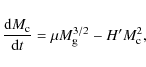
where
Stars form by cloud-cloud interactions at a rate H
and by the interactions of massive stars with clouds at a rate a,
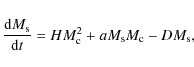
where
5.2 The choice of the stellar yields and the IMF
The model results are sensitive to the assumed stellar yields. For low-
and intermediate-mass stars
(M<8 ![]() ), we used the yields by
Gavilán et al. (2005).
The yields of Marigo (2001)
give comparable results without any appreciable difference in the
computed gradients of chemical elements produced by intermediate mass
stars, such as N with respect to
the gradients computed with the yields by Gavilán et al. (2005).
For stars in the mass range
), we used the yields by
Gavilán et al. (2005).
The yields of Marigo (2001)
give comparable results without any appreciable difference in the
computed gradients of chemical elements produced by intermediate mass
stars, such as N with respect to
the gradients computed with the yields by Gavilán et al. (2005).
For stars in the mass range ![]() we adopt the yields by Chieffi & Limongi (2004). The yields
of more massive stars are affected by the considerable uncertainties
associated with different assumptions about the modelling of processes
like convection, semi-convection, overshooting, and mass loss. Other
difficulties arise from the simulation of the supernova explosion and
the possible fallback after the explosion, that strongly influences the
production of iron-peak elements. It is not surprising then
that the results of different authors (e.g. Arnett 1995; Woosley
& Weaver 1995;
Thielemann et al. 1996;
Aubert
et al. 1996)
disagree in some cases by orders of magnitude. In our models,
we estimate the yields of stars in the mass range
we adopt the yields by Chieffi & Limongi (2004). The yields
of more massive stars are affected by the considerable uncertainties
associated with different assumptions about the modelling of processes
like convection, semi-convection, overshooting, and mass loss. Other
difficulties arise from the simulation of the supernova explosion and
the possible fallback after the explosion, that strongly influences the
production of iron-peak elements. It is not surprising then
that the results of different authors (e.g. Arnett 1995; Woosley
& Weaver 1995;
Thielemann et al. 1996;
Aubert
et al. 1996)
disagree in some cases by orders of magnitude. In our models,
we estimate the yields of stars in the mass range ![]() by linear extrapolation of the
yields in the mass range
by linear extrapolation of the
yields in the mass range ![]() .
.
Another important ingredient in the chemical evolution model is the initial mass function (IMF). Several works support the idea that the IMF is universal in space and constant in time (Wyse 1997; Scalo 1998; Kroupa 2002), apart from local fluctuations. There are several parameterizations of the IMF (see e.g. Romano et al. 2005, for a complete review), starting from, e.g., Salpeter (1955), Tinsley (1980), Scalo (1986), Kroupa et al. (1993), Ferrini et al. (1990), Scalo (1998), Chabrier (2003). In the following, we test the possibility that the observed flat gradients can be explained in terms of a non-standard IMF. In fact, the magnitude and the slope of chemical abundance gradients are related to the number of stars in each mass range, and so to the IMF. The goal is to reproduce, if possible, the flat gradient supported by recent observations by only varying the IMF.
In Fig. 9 we compare the oxygen and nitrogen gradients of H II regions with present-day abundance profiles from the M07b model. The choice of the IMF does not affect the slope of O/H and N/H gradients, but simply shifts the abundance profiles to higher (or lower) values according to the amount of stars that produce oxygen (massive stars) or nitrogen (low- and intermediate-mass stars). With the adopted stellar yields, the best fits of the metallicity distribution of M 33 are obtained with the IMF by Ferrini et al. (1990) and Scalo (1986). For the revised model we thus adopt the parameterization of Ferrini et al. (1990). The different slopes of the O/H and N/H gradients are reproduced fairly well by the chemical evolution model as a natural consequence of the different mass ranges of stellar production, hence timescales, of these two chemical elements (see Sect. 3.2 for a comparison with the measured gradients).
![\begin{figure}
\par\includegraphics[angle=270,width=8cm,clip]{13564fg11.ps}\vspace*{5mm}
\includegraphics[angle=270,width=8cm,clip]{13564fg12.ps}
\end{figure}](/articles/aa/full_html/2010/04/aa13564-09/img56.png)
|
Figure 9: The oxygen ( top panel) and nitrogen ( bottom panel) radial gradients of M07b with several parameterization of the IMF: Salpeter (1955) (continuous green line), Tinsley (1980) (dotted red line), Scalo (1986) (dashed magenta line), Scalo 1998) (long dashed yellow line), Ferrini et al. (1990) (long dash-dotted blue line), Chabrier (2003) (dash-dotted black line). |
| Open with DEXTER | |
5.3 Comparison with the observations
The observational constraints to the model are those described in M07b, complemented with the O/H and N/H radial gradients of H II regions and PNe from this work and M09, respectively, and the radial profile of the SFR determined by Verley et al. (2009) from far ultraviolet (FUV) observations corrected for extinction. For H II regions we used the gradient derived from the whole population (see Eq. (4)), without any distinction in terms of size and brightness, but excluding the central 1 kpc. Giant H II regions might not be representative of the current ISM abundance owing their possible chemical self-enrichment.
In Figs. 10
and 11
we show the radial surface density of molecular gas (from
the single dish observations of Corbelli 2003, averaged
over 1 kpc bins) and the SFR as a function of the
surface density of molecular gas (Verley et al. 2009),
respectively. Both figures show the predictions of the model of M07b at
![]() .
Clearly, the model of M07b in its original formulation is unable to
reproduce these constraints. We have therefore
considered other parameterizations of the star formation process by
varying the radial dependence of the SFE, represented by the
coefficient H.
.
Clearly, the model of M07b in its original formulation is unable to
reproduce these constraints. We have therefore
considered other parameterizations of the star formation process by
varying the radial dependence of the SFE, represented by the
coefficient H.
Our experiments show that, to reproduce the observed behaviour
of the radial gas distribution and the observed Schmidt law,
is necessary to increase the efficiency of star formation at
large
radii. This can be accomplished in many ways. In the previous version
of the model (M07b) H decreased
with
![]() to consider a geometrical correction resulting from how large
galactocentric distances correspond to larger volumes
(see Ferrini et al. 1994).
In the present work we assume that H
is constant with radius, thus implying that the star formation
efficiency increases linearly with galactocentric radius.
In Sect. 5.4
we describe the observational evidence in support this assumption
in M 33.
to consider a geometrical correction resulting from how large
galactocentric distances correspond to larger volumes
(see Ferrini et al. 1994).
In the present work we assume that H
is constant with radius, thus implying that the star formation
efficiency increases linearly with galactocentric radius.
In Sect. 5.4
we describe the observational evidence in support this assumption
in M 33.
![\begin{figure}
\par\includegraphics[angle=270,width=8cm,clip]{13564fg13.ps}
\end{figure}](/articles/aa/full_html/2010/04/aa13564-09/img58.png)
|
Figure 10: The SFR derived from the UV emission corrected for extinction by Verley et al. (2009) vs. the surface density Schmidt law: filled circles (blue) are the molecular gas averaged in bins 1 kpc each (Corbelli 2003; curves represent the model at 0.5 Gyr from the disk formation ( dotted curve), 2 ( dashed curve), 3 ( long-dashed curve), 5 ( dot-dashed curve), 8 ( long dash-dotted curve), 12 ( long-short dashed curve), and at 13.6 Gyr ( solid red curve); the solid green curve is the model by M07b at 13.6 Gyr. |
| Open with DEXTER | |
![\begin{figure}
\par\includegraphics[angle=270,width=8cm,clip]{13564fg14.ps}
\end{figure}](/articles/aa/full_html/2010/04/aa13564-09/img59.png)
|
Figure 11: The radial surface density of molecular gas: filled circles (blue) are the observed molecular gas averaged in bins 1 kpc wide. Model curves have the same symbols as in Fig. 10. |
| Open with DEXTER | |
Assuming that H is spatially constant, we obtain
the results shown in Figs. 10
and 11
at t=0.5, 2, 3, 5, 8, 12, 13.6 Gyr. The
relationship between molecular gas and SFR predicted by the modified
M07b model is more or less constant with time and in good
agreement with the data. The predicted Schmidt law
(at the present time) has an average exponent ![]() ,
in agreement with the observations, whereas the original
M07b model produces a Schmidt law with a higher
exponent,
,
in agreement with the observations, whereas the original
M07b model produces a Schmidt law with a higher
exponent, ![]() .
The better agreement with the observations obtained with the revised
M07b model suggests that M 33 is more efficient in
forming stars than normal local Universe spiral
galaxies, in particular in its outer regions.
.
The better agreement with the observations obtained with the revised
M07b model suggests that M 33 is more efficient in
forming stars than normal local Universe spiral
galaxies, in particular in its outer regions.
5.4 Flat gradients and SF efficiency
Is there evidence of flat gradients in other galaxies? How can they be
explained? A flat gradient in the outer regions of our Galaxy
has been observed by several authors (e.g., Yong et al. 2005; Carraro
et al. 2007;
Sestito et al. 2007)
using different metallicity tracers (e.g., Cepheids, open clusters).
However, other tracers, such as PNe, do not show this behaviour,
indicating flat gradients across the whole disk
(cf. Stanghellini et al. 2006;
Perinotto & Morbidelli 2006).
The outer Galactic plateau might be a phenomenon similar to the flat
gradient of M 33. Since M 33 is less massive than
the MW, its halo collapse phase, responsible for the
steep gradient in the inner regions (
![]() <
11-12 kpc) of our Galaxy (cf. Magrini et al.
2009b),
is less marked. Thus in M 33 the difference between
the inner and outer gradients
is less evident than in the MW. The flat metallicity
distribution of the MW at large radii has been explained with several
chemical evolution models, among them those by Andrievsky
et al. (2004),
Chiappini et al. (2001)
model C, and Magrini et al. (2009b). Andrievsky
et al. (2004)
explain the flat metallicity distribution beyond 11-12 kpc
when assuming that the SFR is a combination of two components: one
proportional to the gas surface density, and the other depending on the
relative velocity of the interstellar gas and spiral arms. With these
assumptions they explain why the breaking point in the slope of the
gradient and the consequent outer flattening, occur around the
co-rotational radius. Chiappini et al. (2001) assume
two main accretion episodes in the lifetime of the Galaxy, the first
one forming the halo and bulge and the second one forming the thin
disk. Their model C is the one able to reproduce a flat
gradient in the external regions, assuming that there is no threshold
in the gas density during the halo/thick-disk phase, and thus allowing
the formation of the outer plateau from infalling gas enriched in the
halo.
Finally, Magrini et al. (2009b)
reproduce the Galactic gradient thanks to the radial dependence of the
infall rate (exponentially decreasing with radius) and with the radial
dependence of the star and cloud formation processes.
To reproduce a completely flat gradient in the outer regions
would, however, require additional accretion of gas uniformly falling
onto the disk, which would result in inconsistent behaviour of the
current SFR.
<
11-12 kpc) of our Galaxy (cf. Magrini et al.
2009b),
is less marked. Thus in M 33 the difference between
the inner and outer gradients
is less evident than in the MW. The flat metallicity
distribution of the MW at large radii has been explained with several
chemical evolution models, among them those by Andrievsky
et al. (2004),
Chiappini et al. (2001)
model C, and Magrini et al. (2009b). Andrievsky
et al. (2004)
explain the flat metallicity distribution beyond 11-12 kpc
when assuming that the SFR is a combination of two components: one
proportional to the gas surface density, and the other depending on the
relative velocity of the interstellar gas and spiral arms. With these
assumptions they explain why the breaking point in the slope of the
gradient and the consequent outer flattening, occur around the
co-rotational radius. Chiappini et al. (2001) assume
two main accretion episodes in the lifetime of the Galaxy, the first
one forming the halo and bulge and the second one forming the thin
disk. Their model C is the one able to reproduce a flat
gradient in the external regions, assuming that there is no threshold
in the gas density during the halo/thick-disk phase, and thus allowing
the formation of the outer plateau from infalling gas enriched in the
halo.
Finally, Magrini et al. (2009b)
reproduce the Galactic gradient thanks to the radial dependence of the
infall rate (exponentially decreasing with radius) and with the radial
dependence of the star and cloud formation processes.
To reproduce a completely flat gradient in the outer regions
would, however, require additional accretion of gas uniformly falling
onto the disk, which would result in inconsistent behaviour of the
current SFR.
Why do we use a radially increasing SFE to reproduce
the flat metallicity gradient of M 33?
M 33 in general is quite different from large spiral galaxies
in terms of SF. A comparison of the SFR to the H2 mass
shows that M 33, like the intermediate redshift galaxies, has
a significantly higher SFE than large local Universe
spirals. There is also observational evidence that the SFE varies with
radius in M 33. Kennicutt (1998b),
Wong & Blitz (2002),
and Murgia et al. (2002)
find a molecular gas depletion timescale (inversely proportional to the
SFE) that varies radially, decreasing by a factor ![]() 2-3. Also
Gardan et al. (2007)
from the CO to SFR ratio also find a dependence of the
depletion timescale on radius, decreasing of a factor
2-3. Also
Gardan et al. (2007)
from the CO to SFR ratio also find a dependence of the
depletion timescale on radius, decreasing of a factor ![]() 2 over
4 kpc. These observations prompted us to model the chemical
evolution of M 33 taking SF processes depending on
radius into account. The general assumption of our model is
that the SF is driven by cloud collisions. Increasing the efficiency of
this process with radius does not imply that cloud-cloud collisions are
more efficient in the outer regions, but that additional processes may
contribute to the SF in the peripheral regions.
2 over
4 kpc. These observations prompted us to model the chemical
evolution of M 33 taking SF processes depending on
radius into account. The general assumption of our model is
that the SF is driven by cloud collisions. Increasing the efficiency of
this process with radius does not imply that cloud-cloud collisions are
more efficient in the outer regions, but that additional processes may
contribute to the SF in the peripheral regions.
5.5 Implications for the metallicity gradient and its evolution
The introduction of more realistic SF process in M 33 has significant consequences on its metallicity gradient and evolution. As described by M09, oxygen modification (destruction or creation) does not occur in the PN population of M 33. Thus oxygen, the best-determined element in nebular optical spectroscopy, can be safely used as a tracer of the ISM composition at the epoch of the formation of PN progenitors. Most PNe in M 33 are older than 0.3 Gyr, and probably much older, up to an age of 10 Gyr.
The metallicity gradient of PNe, including only those with
progenitor stars older than 0.3 Gyr and excluding PNe located
in the first kpc from the centre, is
| (11) |
As discussed above, the whole sample of H II regions is representative of the current ISM composition. The H II region and PN gradients in the same radial region, 1 kpc
In Fig. 12 we show the observed metallicity gradient of M 33 together with the results of the present model (top panel) and of the original model of M07b (bottom panel). For a better comparison, the oxygen abundances of the samples of H II regions and disk PNe have been averaged over bins of 1 kpc each. This allows us to highlight the translation towards the lower metallicity of the PNe. The curves correspond to the present and to 5 Gyr ago (8.6 Gyr from the disk formation, assuming an age of 13.6 Gyr for M 33), i.e., approximately the average period of formation of the PN progenitors. The present model predicts a higher SF in the outer regions, reproducing the observed flatness of the oxygen gradient at large radii better than the M07b model. In addition, the evolution of the metallicity gradient predicted by the new model is consistent with the observations: a negligible change in the slope and a small translation to higher metallicities. Finally, we see that the assumed dependence of the SFE with galactocentric radius, required to reproduce the metallicity evolution of M 33, takes place always as in M07b with a slow building up of the disk of M 33 by accretion from an intergalactic medium or halo gas.
For completeness we also show the N/H radial gradient of the sample of H II regions. For this element the temporal evolution cannot be inferred using PN abundances, since PNe modify their nitrogen composition during their lifetime. The nitrogen abundances have been averaged over bins of 1 kpc each. The observed N/H gradient is significantly steeper than the oxygen gradient, as predicted by the model.
![\begin{figure}
\par\includegraphics[width=8.8cm,clip]{13564fg15.ps}
\end{figure}](/articles/aa/full_html/2010/04/aa13564-09/img64.png)
|
Figure 12: The O/H radial gradient evolution. Top panel: filled circles (blue) are the H II region oxygen abundances from the dataset described in Sect. 2, averaged over radial bins, each 1 kpc wide; filled squares (magenta) are averaged non-type I PN oxygen abundances by M09. The gradient 5 Gyr ago ( dashed curve) and now (continuous curve) as predicted by the present model. Bottom panel: the same as in the top panel but for the accretion model by M07b. |
| Open with DEXTER | |
The time evolution of the metallicity gradient is strictly correlated
to the inside-out growth of the disk. In a recent work,
Williams et al. (2009)
presented the resolved photometry of four fields located at different
galactocentric distances, from 0.9 to 6.1 kpc. Their
photometry provides a detailed census of stellar populations and their
ages at different radii. They find that the percentage of the stellar
mass formed prior to z = 1 (![]() 8 Gyr ago)
changes from
8 Gyr ago)
changes from ![]() 71%
in the innermost field at 0.9 kpc from the centre to
71%
in the innermost field at 0.9 kpc from the centre to ![]() 16% in the
outermost SF region at 6.1 kpc. We thus compare these
results with the cumulative SF predicted by our model at different
ages. The agreement is good in the central field, where model and
observations both have about 70% of the stellar mass already
formed 8 Gyr ago. Also at 2.5 kpc,
corresponding to their second field, the observed stellar mass formed
prior to z = 1 is
about 50% and the model results give 47%. In the
outermost fields, at 4.3 and 6.1 kpc, the agreement
is not as good, since the observations show that 20%
and 16% of stars formed before 8 Gyr ago, while the
model predicts
16% in the
outermost SF region at 6.1 kpc. We thus compare these
results with the cumulative SF predicted by our model at different
ages. The agreement is good in the central field, where model and
observations both have about 70% of the stellar mass already
formed 8 Gyr ago. Also at 2.5 kpc,
corresponding to their second field, the observed stellar mass formed
prior to z = 1 is
about 50% and the model results give 47%. In the
outermost fields, at 4.3 and 6.1 kpc, the agreement
is not as good, since the observations show that 20%
and 16% of stars formed before 8 Gyr ago, while the
model predicts ![]() 44%
for both fields. With the model by M07b, the situation is almost
unvaried in the inner regions, while in the outer regions there is a
slightly lower percentage of stars formed before
8 Gyr ago,
44%
for both fields. With the model by M07b, the situation is almost
unvaried in the inner regions, while in the outer regions there is a
slightly lower percentage of stars formed before
8 Gyr ago, ![]() 33%. The recent evolution of
the outermost SF regions of M 33 can be explained by
an accretion of material in the peripheral regions at recent epochs. In
our model, the scalelength of the disk is constant, and the accretion
in the outer regions is a continuous process. Thus, we are able to
reproduce the integrated SF at any radius and its by-product, the
metallicity, but not to reproduce its temporal behaviour if it is
dominated by stochastic events, such as, e.g., sporadic
massive accretion of gas and tidal interactions. Finally, outside the
SF area of the disk, the age of populations of the outer
disk/halo show an age increase with radius (Barker et al. 2007a,b). This
agrees well with our model results: there is a
slightly larger number of old stars beyond 8 kpc than in the
peripheral part of the SF disk.
33%. The recent evolution of
the outermost SF regions of M 33 can be explained by
an accretion of material in the peripheral regions at recent epochs. In
our model, the scalelength of the disk is constant, and the accretion
in the outer regions is a continuous process. Thus, we are able to
reproduce the integrated SF at any radius and its by-product, the
metallicity, but not to reproduce its temporal behaviour if it is
dominated by stochastic events, such as, e.g., sporadic
massive accretion of gas and tidal interactions. Finally, outside the
SF area of the disk, the age of populations of the outer
disk/halo show an age increase with radius (Barker et al. 2007a,b). This
agrees well with our model results: there is a
slightly larger number of old stars beyond 8 kpc than in the
peripheral part of the SF disk.
![\begin{figure}
\par\includegraphics[width=8.8cm,clip]{13564fg16.ps}
\end{figure}](/articles/aa/full_html/2010/04/aa13564-09/img65.png)
|
Figure 13: The N/H radial gradient. Top panel: filled circles (blue) are the H II region nitrogen abundances from the dataset described in Sect. 2, averaged over radial bins, each 1 kpc wide. The gradient at the present time as predicted by the present model is the continuous curve. Bottom panel: the same as in the top panel but for the accretion model by M07b. |
| Open with DEXTER | |
6 Summary and conclusions
We have studied the chemical evolution of M 33 by means of new
spectroscopic observations of H II regions,
together with literature data of H II regions
and PNe. We derived the radial oxygen gradient in the range
from 1 to ![]() 8 kpc.
Its slope is -0.044
8 kpc.
Its slope is -0.044 ![]() 0.009 dex kpc-1. We excluded
the central 1 kpc region from the gradient because of its low
metallicity. In fact, the 2D metallicity map is
off-centre, with a peak in the southern arm at 1-2 kpc from
the centre. We measured the highest metallicity gradient in bright
regions which are not located in the centre of M 33.
We explained this effect with a bias in the measurement of nebular
abundances towards low metallicity in the central regions and/or with
SF bursts which had not had time to mix azimuthally.
At a galactocentric distance of about 1.5 kpc, the
spread of metal abundances is much greater than the dispersion along
the average gradient, and it is possibly related to the presence
of a bar.
0.009 dex kpc-1. We excluded
the central 1 kpc region from the gradient because of its low
metallicity. In fact, the 2D metallicity map is
off-centre, with a peak in the southern arm at 1-2 kpc from
the centre. We measured the highest metallicity gradient in bright
regions which are not located in the centre of M 33.
We explained this effect with a bias in the measurement of nebular
abundances towards low metallicity in the central regions and/or with
SF bursts which had not had time to mix azimuthally.
At a galactocentric distance of about 1.5 kpc, the
spread of metal abundances is much greater than the dispersion along
the average gradient, and it is possibly related to the presence
of a bar.
We analysed and discussed the metallicity gradient of giant H II regions, i.e. the largest regions with high surface brightness. We find it steeper than the average of the sample gradient, in agreement with the early spectroscopic studies of H II regions in M 33, based mainly on the brightest objects.
We compared the metallicity gradients of H II regions and of PNe, obtained with the same set of observations and analysis techniques. We find a substantially unchanged slope of the gradient, and an overall increase in metallicity with time. We can explain the slow evolution of the metallicity gradient from the present to the birth of the PN progenitors with a chemical evolution accretion model, as in M07b, if the SFE is higher at larger radii.
Appendix A: Comparison with the literature
To assess the quality of the MMT observations we compared the oxygen
abundance in the control sample with those available in the literature.
Oxygen is in fact the most widely used element in emission-line optical
spectroscopy because it gives accurate results for determining the
metallicity. This is because i) many ionization stages are
present in the optical range ([O I],
[O II], [O III]),
and the corrections for unseen ionization stages are often not needed;
ii) a direct measurement of its electron
temperatures, ![]() [O III]
and
[O III]
and ![]() [O II],
is possible. For each source in the control sample, we show in
Table A.1
the oxygen abundance determined by different authors (Rosolowsky
& Simon 2008;
Magrini et al. 2007a;
Crockett et al. 2006;
Vilchez et al. 1988;
Kwitter & Aller 1981)
and in this paper. In Cols. 2 to 6 we report
the literature O/H and our measurements
in Col. 7. For H II regions
with multiple determinations we computed the weighted average of all
measurements. The agreement is reasonably good for all sources, since
our values are consistent, within the errors, with those available in
the literature. The average O/H abundance of the
14 H II regions
agrees. The average dispersion between our values and previous
determinations is only 0.09 dex.
[O II],
is possible. For each source in the control sample, we show in
Table A.1
the oxygen abundance determined by different authors (Rosolowsky
& Simon 2008;
Magrini et al. 2007a;
Crockett et al. 2006;
Vilchez et al. 1988;
Kwitter & Aller 1981)
and in this paper. In Cols. 2 to 6 we report
the literature O/H and our measurements
in Col. 7. For H II regions
with multiple determinations we computed the weighted average of all
measurements. The agreement is reasonably good for all sources, since
our values are consistent, within the errors, with those available in
the literature. The average O/H abundance of the
14 H II regions
agrees. The average dispersion between our values and previous
determinations is only 0.09 dex.
Table A.1: Comparison of oxygen measurements of our control sample with literature O/H.
AcknowledgementsWe warmly thank J. Vilchez for interesting discussion on the argument. We thank R. Walterbos for allowing us to use his Hcalibrated map of M 33. We thank D. Fabricant for making Hectospec available to the community, and the Hectospec instrument team and MMT staff for their expert help in preparing and carrying out the Hectospec observing runs. We thank N. Caldwell, D. Ming, and their team for the help during the data reduction. L.S. acknowledges the hospitality of the Observatoire de Paris where a part of this work was developed.
References
- Afflerbach, A., Churchwell, E., & Werner, M. W. 1997, ApJ, 478, 190 [NASA ADS] [CrossRef] [Google Scholar]
- Andrievsky, S. M., Luck, R. E., Martin, P., & Lèpine, J. R. D. 2004, A&A, 413, 159 [NASA ADS] [CrossRef] [EDP Sciences] [Google Scholar]
- Arnett, D. 1995 ARA&A, 33, 115 [Google Scholar]
- Asplund, M., Grevesse, N., & Sauval, A. J. 2005, ASPC, 336, 25 [Google Scholar]
- Aubert, O., Prantzos, N., & Baraffe, I. 1996, A&A, 312, 845 [NASA ADS] [Google Scholar]
- Barker, M. K., Sarajedini, A., Geisler, D., Harding, P., & Schommer, R. 2007a, AJ, 133, 1125 [NASA ADS] [CrossRef] [Google Scholar]
- Barker, M. K., Sarajedini, A., Geisler, D., Harding, P., & Schommer, R. 2007b, AJ, 133, 1138 [NASA ADS] [CrossRef] [Google Scholar]
- Benjamin, R. A., Skillman, E. D., & Smits, D. P. 1999, ApJ, 514, 307 [NASA ADS] [CrossRef] [Google Scholar]
- Bonanos, A. Z., Stanek, K. Z., Kudritzki, R. P., et al. 2006, ApJ, 652, 313 [NASA ADS] [CrossRef] [Google Scholar]
- Boulesteix, J., Courtes, G., Laval, A., Monnet, G., & Petit, H. 1974, A&A, 37, 33 [NASA ADS] [Google Scholar]
- Bresolin, F. 2007, ApJ, 656, 186 [NASA ADS] [CrossRef] [Google Scholar]
- Bresolin, F., Gieren, W., Kudritzki, R.-P., et al. 2009, ApJ, 700, 309 [NASA ADS] [CrossRef] [Google Scholar]
- Brunthaler, A., Reid, M. J., Falcke, H., Greenhill, L. J., & Henkel, C. 2005, Science, 307, 1440 [NASA ADS] [CrossRef] [PubMed] [Google Scholar]
- Chabrier, G. 2003, PASP, 115, 763 [NASA ADS] [CrossRef] [Google Scholar]
- Chiappini, C., Matteucci, F., & Romano, D. 2001, ApJ, 554, 1044 [NASA ADS] [CrossRef] [Google Scholar]
- Chieffi, A., & Limongi, M. 2004, ApJ, 608, 405 [NASA ADS] [CrossRef] [Google Scholar]
- Carraro, G., Geisler, D., Villanova, S., Frinchaboy, P. M., & Majewski, S. R. 2007, A&A, 476, 217 [NASA ADS] [CrossRef] [EDP Sciences] [Google Scholar]
- Clegg, R. E. S. 1987, MNRAS, 229, 31 [NASA ADS] [CrossRef] [Google Scholar]
- Colin, J., & Athanassoula, E. 1981, A&A, 97, 63 [NASA ADS] [Google Scholar]
- Corbelli, E. 2003, MNRAS, 342, 199 [NASA ADS] [CrossRef] [Google Scholar]
- Corbelli, E., & Walterbos, R. A. M. 2007, ApJ, 669, 315 [NASA ADS] [CrossRef] [Google Scholar]
- Corradi, R. L. M., & Magrini, L. 2006, in Planetary Nebulae Beyond the Milky Way, ESO Astrophys. Symp., 36 [Google Scholar]
- Courtes, G., Petit, H., Petit, M., Sivan, J.-P., & Dodonov, S. 1987, A&A, 174, 28 [NASA ADS] [Google Scholar]
- Crockett, N. R., Garnett, D. R., Massey, P., & Jacoby, G. 2006, ApJ, 637, 741 [NASA ADS] [CrossRef] [Google Scholar]
- Devereux, N., Duric, N., & Scowen, P. A. 1997, AJ, 113, 236 [NASA ADS] [CrossRef] [Google Scholar]
- Dopita, M. A. 1991, IAUS, 148, 393 [NASA ADS] [Google Scholar]
- Engargiola, G., Plambeck, R. L., Rosolowsky, E., & Blitz, L. 2003, ApJS, 149, 343 [NASA ADS] [CrossRef] [Google Scholar]
- Fabricant, D., Fata, R., Roll, J., et al. 2005, PASP, 117, 1411 [NASA ADS] [CrossRef] [Google Scholar]
- Ferrini, F., Penco, U., & Palla, F. 1990, A&A, 231, 391 [NASA ADS] [Google Scholar]
- Ferrini, F., Matteucci, F., Pardi, C., & Penco, U. 1992, ApJ, 387, 138 [NASA ADS] [CrossRef] [Google Scholar]
- Ferrini, F., Mollá, M., Pardi, M. C., & Diaz, A. I. 1994, ApJ, 427, 745 [NASA ADS] [CrossRef] [Google Scholar]
- Freedman, W. L., Wilson, C. D., & Madore, B. F. 1991, ApJ, 372, 455 [NASA ADS] [CrossRef] [Google Scholar]
- Gardan, E., Braine, J., Schuster, K. F., Brouillet, N., & Sievers, A. 2007, A&A, 473, 91 [NASA ADS] [CrossRef] [EDP Sciences] [Google Scholar]
- Garnett, D. R., Shields, G. A., Skillman, E. D., Sagan, S. P., & Dufour, R. J. 1997, ApJ, 489, 63 [NASA ADS] [CrossRef] [Google Scholar]
- Gavilán, M., Buell, J. F., & Mollá, M. 2005, A&A, 432, 861 [NASA ADS] [CrossRef] [EDP Sciences] [Google Scholar]
- Gordon, S. M., Duric, N., Kirchner, R. P., Goss, W. M., & Viallefond, F. 1999, ApJS, 120, 247 [NASA ADS] [CrossRef] [Google Scholar]
- Herrero, A., Lennon, D. J., Vílchez, J. M., Kudritzki, R. P., & Humphreys, R. H. 1994, A&A, 287, 885 [NASA ADS] [Google Scholar]
- Holmberg, E. 1958, Lund Medd. Astron. Obs. Ser. II, 136, 1 [NASA ADS] [Google Scholar]
- Kennicutt, R. C. 1998, ApJ, 498, 541 [NASA ADS] [CrossRef] [Google Scholar]
- Kennicutt, R. C., Jr. 1998, ARA&A, 36, 189 [Google Scholar]
- Kingsburgh, R. L., & Barlow, M. J. 1994, MNRAS, 271, 257 [NASA ADS] [CrossRef] [Google Scholar]
- Kroupa, P. 2002, Science, 295, 82 [NASA ADS] [CrossRef] [PubMed] [Google Scholar]
- Kroupa, P., Tout, C. A., & Gilmore, G. 1993, MNRAS, 262, 545 [NASA ADS] [CrossRef] [Google Scholar]
- Kwitter, K. B., & Aller, L. H. 1981, MNRAS, 195, 939 [NASA ADS] [Google Scholar]
- Magrini, L., Vilchez, J. M., Mampaso, A., Corradi, R. L. M., & Leisy, P. 2007a, A&A, 470, 865 (M07a) [NASA ADS] [CrossRef] [EDP Sciences] [Google Scholar]
- Magrini, L., Corbelli, E., & Galli, D. 2007b, A&A, 470, 843 (M07b) [NASA ADS] [CrossRef] [EDP Sciences] [Google Scholar]
- Magrini, L., Stanghellini, L., & Villaver, E. 2009a, ApJ, 696, 729 (M09) [NASA ADS] [CrossRef] [Google Scholar]
- Magrini, L., Sestito, P., Randich, S., & Galli, D. 2009b, A&A, 494, 95 [NASA ADS] [CrossRef] [EDP Sciences] [Google Scholar]
- Marigo, P. 2001, A&A, 370, 194 [NASA ADS] [CrossRef] [EDP Sciences] [Google Scholar]
- Maraston, C. 2005, MNRAS, 362, 799 [NASA ADS] [CrossRef] [Google Scholar]
- Massey, P., & Johnson, O. 1998, ApJ, 505, 793 [NASA ADS] [CrossRef] [Google Scholar]
- Massey, P., Strobel, K., Barnes, J. V., & Anderson, E. 1988, ApJ, 328, 315 [NASA ADS] [CrossRef] [Google Scholar]
- Mathis, J. S. 1990, ARA&A, 28, 37 [NASA ADS] [CrossRef] [Google Scholar]
- McCarthy, J. K., Lennon, D. J., Venn, K. A., & Kudritzki, R.-P. 1995, ApJ, 455, 135 [NASA ADS] [CrossRef] [Google Scholar]
- Minniti, D., Olszewski, E. W., & Rieke, M. 1993, ApJ, 410, L79 [NASA ADS] [CrossRef] [Google Scholar]
- Monteverde, M. I., Herrero, A., Lennon, D. J., & Kudritzki, R.-P. 1997, ApJ, 474, 107 [NASA ADS] [CrossRef] [Google Scholar]
- Monteverde, M. I., Herrero, A., & Lennon, D. J. 2000, ApJ, 545, 813 [NASA ADS] [CrossRef] [Google Scholar]
- Murgia, M., Crapsi, A., Moscadelli, L., & Gregorini, L. 2002, A&A, 385, 412 [NASA ADS] [CrossRef] [EDP Sciences] [Google Scholar]
- Nagao, T., Maiolino, R., & Marconi, A. 2006, A&A, 459, 85 [NASA ADS] [CrossRef] [EDP Sciences] [Google Scholar]
- Osterbrock, D. E., & Ferland, G. J. 2006, Astrophysics of Gaseous Nebulae and Active Galactic Nuclei, 2nd. edn., ed. D. E. Osterbrock, & G. J. Ferland (Sausalito, CA: University Science Books), Sky and Telescope, 78 [Google Scholar]
- Perinotto, M., & Morbidelli, L. 2006, MNRAS, 372, 45 [NASA ADS] [CrossRef] [Google Scholar]
- Press, W. H., Teukolsky, S. A., Vetterling, W. T., & Flannery, B. F. 1992, Numerical Recipes in FORTRAN: The art of scientific computing, 2nd edn. [Google Scholar]
- Regan, M. W., & Vogel, S. N. 1994, ApJ, 434, 536 [NASA ADS] [CrossRef] [Google Scholar]
- Relaño, M., & Kennicutt, R. C. 2009, ApJ, 699, 1125 [NASA ADS] [CrossRef] [Google Scholar]
- Romano, D., Chiappini, C., Matteucci, F., & Tosi, M. 2005, A&A, 430, 491 [NASA ADS] [CrossRef] [EDP Sciences] [Google Scholar]
- Rosolowsky, E., & Simon, J. D. 2008, ApJ, 675, 1213 [NASA ADS] [CrossRef] [Google Scholar]
- Rubin, R. H., Simpson, J. P., Colgan, S. W. J., et al. 2008, MNRAS, 387, 45 [NASA ADS] [CrossRef] [Google Scholar]
- Salpeter, E. E. 1955, ApJ, 121, 161 [Google Scholar]
- Sarajedini, A., Barker, M. K., Geisler, D., Harding, P. & Schommer, R. 2006, AJ, 132, 1361 [NASA ADS] [CrossRef] [Google Scholar]
- Scalo, J. 1986, Fundamentals of Cosmic Physics, 11, 1 [Google Scholar]
- Scalo, J. 1998, ASPC, 142, 201 [Google Scholar]
- Schmidt, M. 1959, ApJ, 129, 243 [NASA ADS] [CrossRef] [Google Scholar]
- Searle, L. 1971, ApJ, 168, 327 [NASA ADS] [CrossRef] [Google Scholar]
- Sestito, P., Randich, S., & Bragaglia, A. 2007, A&A, 465, 185 [NASA ADS] [CrossRef] [EDP Sciences] [Google Scholar]
- Skrutskie, M. F., Cutri, R. M., Stiening, R., et al. 2006, AJ, 131, 1163 [NASA ADS] [CrossRef] [Google Scholar]
- Simon, J. D., & Rosolowsky, E. 2008, ASPC, 396, 23 [NASA ADS] [Google Scholar]
- Shaw, R. A., & Dufour, R. J. 1994, ASPC, 61, 327 [Google Scholar]
- Smith, H. E. 1975, ApJ, 199, 591 [NASA ADS] [CrossRef] [Google Scholar]
- Stasinska, G. 2005, A&A, 434, 507 [NASA ADS] [CrossRef] [EDP Sciences] [Google Scholar]
- Stanghellini, L., Guerrero, M. A., Cunha, K., Manchado, A., & Villaver, E. 2006, ApJ, 651, 898 [NASA ADS] [CrossRef] [Google Scholar]
- Stephens, A. W., & Frogel, J. A. 2002, AJ, 124, 2023 [NASA ADS] [CrossRef] [Google Scholar]
- Thielemann, F.-K., Nomoto, K., & Hashimoto, M.-A. 1996, ApJ, 460, 408 [NASA ADS] [CrossRef] [Google Scholar]
- Tinsley, B. M. 1981, Fundamentals of Cosmic Physics, 5, 287 [Google Scholar]
- Thilker, D. A., Hoopes, C. G., Bianchi, L., et al. 2005, ApJ, 619, L67 [NASA ADS] [CrossRef] [Google Scholar]
- Urbaneja, M. A., Herrero, A., Kudritzki, R.-P., et al. 2005, ApJ, 635, 311 [NASA ADS] [CrossRef] [Google Scholar]
- Vivian, U., Urbaneja, M. A., Kudritzki, R.-P., et al. 2009, ApJ, 704, 1120 [NASA ADS] [CrossRef] [Google Scholar]
- Venn, K. A., McCarthy, J. K., Lennon, D. J., & Kudritzki, R. P. 1998, ASPC, 147, 54 [NASA ADS] [Google Scholar]
- Verley, S., Corbelli, E., Giovanardi, C., & Hunt, L. K. 2009, A&A, 493, 453 [NASA ADS] [CrossRef] [EDP Sciences] [Google Scholar]
- Vílchez, J. M., Pagel, B. E. J., Diaz, A. I., Terlevich, E., & Edmunds, M. G. 1988, MNRAS, 235, 633 [NASA ADS] [CrossRef] [Google Scholar]
- Williams, B. F., Dalcanton, J. J., Dolphin, A. E., Holtzman, J., & Sarajedini, A. 2009, ApJ, 695, L15 [NASA ADS] [CrossRef] [Google Scholar]
- Willner, S. P., & Nelson-Patel, K. 2002, ApJ, 598, 679 [NASA ADS] [CrossRef] [Google Scholar]
- Wilson, C. D., & Scoville, N. 1989, ApJ, 347, 743 [NASA ADS] [CrossRef] [Google Scholar]
- Wong, T., & Blitz, L. 2002, ApJ, 569, 157 [NASA ADS] [CrossRef] [Google Scholar]
- Woosley, S. E., & Weaver, T. A. 1995, ApJS, 101, 181 [NASA ADS] [CrossRef] [Google Scholar]
- Wyse, R. F. G. 1997, ApJ, 490, 69 [NASA ADS] [CrossRef] [Google Scholar]
- Yong, D., Carney, B. W., & de Almeida, L. 2005, AJ, 130, 597 [NASA ADS] [CrossRef] [Google Scholar]
Footnotes
- ... variations
- Full Tables 2 and 3 are only available in electronic form at the CDS via anonymous ftp to cdsarc.u-strasbg.fr (130.79.128.5) or via http://cdsweb.u-strasbg.fr/cgi-bin/qcat?J/A+A/512/A63
- ... IRAF
- IRAF is distributed by the National Optical Astronomy Observatory, which is operated by the Association of Universities for Research in Astronomy (AURA) under cooperative agreement with the National Science Foundation.
All Tables
Table 1: MMT observations of H II regions with chemical abundance determination.
Table 2: Observed and de-reddened fluxes (full table available at the CDS).
Table 3: Plasma diagnostics and abundances (full table available at the CDS).
Table 4: The chemical abundances of our MMT sample.
Table 5: The radial gradients of N/H, Ne/H, S/H and Ar/H.
Table 6: Giant H II regions with derived chemical abundances.
Table 7:
H II regions in the central
regions without direct ![]() measurement.
measurement.
Table A.1: Comparison of oxygen measurements of our control sample with literature O/H.
All Figures
|
|
Figure 1:
Two example spectra of H II
regions located at different galactocentric distance:
BCLMP 694 at |
| Open with DEXTER | |
| In the text | |
|
|
Figure 2: The O/H radial gradient for the cumulative H II region sample: filled circles are the MMT observations (new and control samples), empty circles are the literature abundances. The continuous line is the weighted linear least-square fit of Eq. (3), i.e., with a radial range from 1 to 8 kpc from the M 33 centre. The dashed vertical line indicates the regions located at its left-side and excluded from the fit. |
| Open with DEXTER | |
| In the text | |
|
|
Figure 3: The O/H radial gradient obtained in different regions of M 33. Top: nearest side (filled squares) and farthest side (empty squares) gradient. Bottom: North (filled squares) and South (empty squares) gradient. In each panel the weighted linear least-square fits of the two regions are shown with two lines (continuous and dotted). |
| Open with DEXTER | |
| In the text | |
|
|
Figure 4: The O/H radial gradient: the giant H II regions (empty triangles) and the complete sample averaged in bins, each 1 kpc wide (filled squares). The continuous line is the weighted mean least square fit of the giant H II region sample, while the dotted line refers to the complete sample. |
| Open with DEXTER | |
| In the text | |
|
|
Figure 5:
The oxygen abundance maps of M 33 (60 |
| Open with DEXTER | |
| In the text | |
|
|
Figure 6: The O/H radial gradient computed with the centre located at RA 1:33:59 dec 30:33:35 (J2000.0) to minimize the dispersion in the slope of the radial gradient. |
| Open with DEXTER | |
| In the text | |
|
|
Figure 7:
The radial gradient of |
| Open with DEXTER | |
| In the text | |
|
|
Figure 8:
The O/H radial gradient: the symbols for the H II regions
with a positive detection of |
| Open with DEXTER | |
| In the text | |
|
|
Figure 9: The oxygen ( top panel) and nitrogen ( bottom panel) radial gradients of M07b with several parameterization of the IMF: Salpeter (1955) (continuous green line), Tinsley (1980) (dotted red line), Scalo (1986) (dashed magenta line), Scalo 1998) (long dashed yellow line), Ferrini et al. (1990) (long dash-dotted blue line), Chabrier (2003) (dash-dotted black line). |
| Open with DEXTER | |
| In the text | |
|
|
Figure 10: The SFR derived from the UV emission corrected for extinction by Verley et al. (2009) vs. the surface density Schmidt law: filled circles (blue) are the molecular gas averaged in bins 1 kpc each (Corbelli 2003; curves represent the model at 0.5 Gyr from the disk formation ( dotted curve), 2 ( dashed curve), 3 ( long-dashed curve), 5 ( dot-dashed curve), 8 ( long dash-dotted curve), 12 ( long-short dashed curve), and at 13.6 Gyr ( solid red curve); the solid green curve is the model by M07b at 13.6 Gyr. |
| Open with DEXTER | |
| In the text | |
|
|
Figure 11: The radial surface density of molecular gas: filled circles (blue) are the observed molecular gas averaged in bins 1 kpc wide. Model curves have the same symbols as in Fig. 10. |
| Open with DEXTER | |
| In the text | |
|
|
Figure 12: The O/H radial gradient evolution. Top panel: filled circles (blue) are the H II region oxygen abundances from the dataset described in Sect. 2, averaged over radial bins, each 1 kpc wide; filled squares (magenta) are averaged non-type I PN oxygen abundances by M09. The gradient 5 Gyr ago ( dashed curve) and now (continuous curve) as predicted by the present model. Bottom panel: the same as in the top panel but for the accretion model by M07b. |
| Open with DEXTER | |
| In the text | |
|
|
Figure 13: The N/H radial gradient. Top panel: filled circles (blue) are the H II region nitrogen abundances from the dataset described in Sect. 2, averaged over radial bins, each 1 kpc wide. The gradient at the present time as predicted by the present model is the continuous curve. Bottom panel: the same as in the top panel but for the accretion model by M07b. |
| Open with DEXTER | |
| In the text | |
Copyright ESO 2010
Current usage metrics show cumulative count of Article Views (full-text article views including HTML views, PDF and ePub downloads, according to the available data) and Abstracts Views on Vision4Press platform.
Data correspond to usage on the plateform after 2015. The current usage metrics is available 48-96 hours after online publication and is updated daily on week days.
Initial download of the metrics may take a while.