| Issue |
A&A
Volume 512, March-April 2010
|
|
|---|---|---|
| Article Number | A28 | |
| Number of page(s) | 5 | |
| Section | The Sun | |
| DOI | https://doi.org/10.1051/0004-6361/200913478 | |
| Published online | 25 March 2010 | |
Time damping of non-adiabatic magnetohydrodynamic waves in a partially ionized prominence plasma: effect of helium
R. Soler - R. Oliver - J. L. Ballester
Departament de Física, Universitat de les Illes Balears, 07122 Palma de Mallorca, Spain
Received 15 October 2009 / Accepted 14 December 2009
Abstract
Context. Prominences are partially ionized, magnetized
plasmas embedded in the solar corona. Damped oscillations and
propagating waves are commonly observed. These oscillations have been
interpreted in terms of magnetohydrodynamic (MHD) waves. Ion-neutral
collisions and non-adiabatic effects (radiation losses and thermal
conduction) have been proposed as damping mechanisms.
Aims. We study the effect of the presence of helium on the time
damping of non-adiabatic MHD waves in a plasma composed by electrons,
protons, neutral hydrogen, neutral helium (He I), and singly ionized helium (He II) in the single-fluid approximation.
Methods. The dispersion relation of linear non-adiabatic MHD
waves in a homogeneous, unbounded, and partially ionized prominence
medium is derived. We compute the period and the damping time of
Alfvén, slow, fast, and thermal waves. A parametric study of the ratio
of the damping time to the period with respect to the helium abundance
is performed.
Results. The efficiency of ion-neutral collisions, as well as
thermal conduction, is increased by the presence of helium. However, if
realistic abundances of helium in prominences (![]() 10%) are considered, this has a minor influence on the wave damping.
10%) are considered, this has a minor influence on the wave damping.
Conclusions. The presence of helium can be safely neglected in studies of MHD waves in partially ionized prominence plasmas.
Key words: Sun: oscillations - magnetic fields - Sun: corona - Sun filaments, prominences
1 Introduction
Small-amplitude oscillations and propagating waves are commonly observed in both quiescent and active region prominences/filaments. They have been interpreted in terms of magnetohydrodynamic (MHD) eigenmodes of the magnetic structure and/or propagating MHD waves. The reader is referred to some recent reviews for more information about the observational and theoretical backgrounds (Engvold 2008,2004; Banerjee et al. 2007; Ballester 2006; Oliver & Ballester 2002).
Prominence oscillations are known to be quickly damped, with damping times corresponding to a few oscillatory periods (reviewed by Mackay et al. 2010; Oliver 2009). Several damping mechanisms of MHD waves have been proposed, with non-adiabatic effects and ion-neutral collisions the more extensively investigated. To understand these effects in detail, they have been studied in simple configurations such as unbounded and homogeneous media. Carbonell et al. (2004) investigated the time damping in a homogeneous prominence medium taking non-adiabatic effects (optically thin radiation losses and thermal conduction) into account. Later on, the spatial damping was studied by Carbonell et al. (2006) and the effect of a background mass flow was analyzed by Carbonell et al. (2009). Subsequently, some works have extended these previous results by considering the presence of the coronal medium (Soler et al. 2009a,2007,2008). The common conclusion of these investigations is that only slow and thermal waves are efficiently damped by non-adiabatic effects, while fast waves are very slightly damped and Alfvén waves are completely unaffected.
On the other hand, the influence of partial ionization on the propagation and time damping of MHD waves has been also investigated in an unbounded medium. Forteza et al. (2007) follow the treatment by Braginskii (1965) to derive the full set of MHD equations along with the dispersion relation of linear waves in a partially ionized, single-fluid plasma (see also Pinto et al. 2008). The electrons, protons, and neutral hydrogen atoms were taken into account, whereas helium and other species were not considered. In a subsequent work (Forteza et al. 2008), they extended their previous analysis by considering radiative losses and thermal conduction by electrons and neutrals. Their main results with respect to the fully ionized case (Carbonell et al. 2004) were, first of all, that ion-neutral collisions (by means of the so-called Cowling's diffusion) can damp both Alfvén and fast waves but non-adiabatic effects remain only important for the damping of slow and thermal waves, and second, that critical values of the wavenumber exist in which the real part of the frequency vanishes, so wave propagation is impossible for larger wavenumbers. Again, applications to a more complex cylindrical geometry have also been performed (Soler et al. 2009c,b).
On the basis of these previous results, it seems clear that partial ionization plays a relevant role on wave propagation in prominences. Prominences are roughly composed of 90% hydrogen and 10% helium but, to date, all the investigations considered a pure hydrogen plasma. Therefore, the effect of the helium on the propagation and damping of MHD waves is still unknown and is the motivation for the present work. Here, we consider an unbounded and homogeneous prominence medium permeated by a homogeneous magnetic field. The plasma is assumed to be partially ionized, because electrons, protons, neutral hydrogen, neutral helium (He I), and singly ionized helium (He II) are the species taken into account. Recent studies by Gouttebroze & Labrosse (2009) indicate that, for central prominence temperatures, the ratio of the number densities of He II to He I is around 10%, whereas the presence of He III is negligible. This result allows us to neglect He III in this work. Extending the works by Forteza et al. (2008,2007), the derivation of the basic MHD equations for a non-adiabatic, partially ionized, single-fluid plasma has been generalized by now considering five different species, allowing us to study how the presence of neutral and singly ionized helium affects their previous results.
This paper is organized as follows. The description of the equilibrium and the basic equations are given in Sect. 2. The results are discussed in Sect. 3. Finally, Sect. 4 contains the conclusion of this work.
2 Equilibrium and basic equations
Our equilibrium configuration is a homogeneous and unbounded partially ionized plasma composed by electrons, protons, neutral hydrogen, neutral helium, and singly ionized helium. Hereafter, subscripts e, p, H, He I, and He II explicitly denote these species, respectively. The magnetic field is also homogeneous and orientated along the x-direction,
|
(1) |
with
| (2) |
|
(3) |
Since

|
(4) |
where R is the ideal gas constant and
|
(5) |
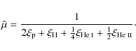
We can express
![\begin{displaymath}\tilde{\mu}= \frac{\tilde{\mu}_{\rm H}}{1- \left[\left( 1 + \...
...ilde{\mu}_{\rm H}\right] \xi_{\mbox{\scriptsize He {\sc i}}}},
\end{displaymath}](/articles/aa/full_html/2010/04/aa13478-09/img32.png)
here we have defined

|
(7) |
The quantity
![\begin{figure}
\par\includegraphics[width=7.5cm]{13478f1.eps}
\end{figure}](/articles/aa/full_html/2010/04/aa13478-09/img45.png)
|
Figure 1:
Mean atomic weight,
|
| Open with DEXTER | |
The details of the derivation of the basic governing equations for a
non-adiabatic, partially ionized, one-fluid plasma can be followed in,
e.g., Braginskii (1965), Forteza et al. (2008,2007), Pinto et al. (2008). Here, we follow the same procedure but generalize the analysis of Forteza et al. (2007)
by including additional species. In brief, the separate governing
equations for the five species are added and a generalized Ohm's law is
obtained. A key step in the present derivation is to compute the
density current, ![]() ,
as
,
as

|
(8) |
along with the condition

![\begin{displaymath}\frac{{\rm D} p}{{\rm D} t} - \frac{\gamma p}{\rho} \frac{{\r...
...dot \left( \mathbf{\kappa} \cdot \nabla T \right) \right] = 0,
\end{displaymath}](/articles/aa/full_html/2010/04/aa13478-09/img54.png)
| (13) |

where

Thus, Ohm's and Cowling's conductivities, as well as the diamagnetic current coefficient,
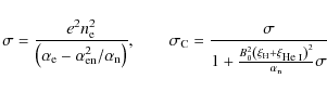

|
(17) |
In addition,
| (18) |
| (19) |
| (20) |
Each particular friction coefficient,
| (21) |
with
|
(22) |
with

|
(23) |
with
|
(24) |
with
| Figure 2:
Ratio of the damping time to the period,
|
|
| Open with DEXTER | |
| Figure 3:
Ratio of the damping time to the period,
|
|
| Open with DEXTER | |
On the other hand, the thermal conductivity due to neutrals (Eq. (16) of Forteza et al. 2008) now has to include the helium contribution. According to Parker (1953), a corrected expression for the conductivity of neutrals in MKS units is
Finally, we assume an optically thin radiation (Hildner 1974) to represent the hydrogen radiative losses. According to Cox & Tucker (1969, see their Fig. 3), the radiative losses by helium are several orders of magnitude less than those of hydrogen for typical prominence temperatures (
Hereafter, our analysis follows that of Forteza et al. (2008). We linearize the basic equations and assume small perturbations proportional to
![]() .
Then the resulting equations (Eq. (18)-(27) of Forteza et al. 2008)
are combined and finally two different, uncoupled dispersion relations,
one for Alfvén waves (their Eq. (28)) and another for
magnetoacoustic and thermal waves (their Eq. (30)), are obtained.
Although our definitions of
.
Then the resulting equations (Eq. (18)-(27) of Forteza et al. 2008)
are combined and finally two different, uncoupled dispersion relations,
one for Alfvén waves (their Eq. (28)) and another for
magnetoacoustic and thermal waves (their Eq. (30)), are obtained.
Although our definitions of ![]() ,
,
![]() ,
,
![]() ,
and
,
and
![]() contain the effect of helium, the resulting dispersion relations are formally identical to those of Forteza et al. (2008).
For the sake of simplicity, we do not write these expressions here
again and refer the reader to that paper. The dispersion relations are
numerically solved for real values of the wavenumber modulus,
contain the effect of helium, the resulting dispersion relations are formally identical to those of Forteza et al. (2008).
For the sake of simplicity, we do not write these expressions here
again and refer the reader to that paper. The dispersion relations are
numerically solved for real values of the wavenumber modulus,
![]() ,
and the angle
,
and the angle ![]() between
between ![]() and
and ![]() .
A complex frequency,
.
A complex frequency,
![]() ,
is obtained. The period, P, and damping time,
,
is obtained. The period, P, and damping time,
![]() ,
are related to the real and imaginary parts of the frequency as
,
are related to the real and imaginary parts of the frequency as
|
(26) |
3 Results
In the following computations, unless otherwise stated, we consider typical quiescent prominence conditions,
![]() kg m-3, T=8000 K, and B0 = 5 G. Quantities
kg m-3, T=8000 K, and B0 = 5 G. Quantities
![]() ,
,
![]() ,
and
,
and
![]() are considered free parameters. We focus our attention on the effect of the relative neutral helium density,
are considered free parameters. We focus our attention on the effect of the relative neutral helium density,
![]() ,
on the ratio
,
on the ratio
![]() .
.
3.1 Free propagation in an unbounded medium
First, we assume
![]() .
Figure 2 displays
.
Figure 2 displays
![]() as a function of k
for the Alfvén, fast, and slow waves. The results corresponding to
several helium abundances are compared for hydrogen and helium
ionization degrees of
as a function of k
for the Alfvén, fast, and slow waves. The results corresponding to
several helium abundances are compared for hydrogen and helium
ionization degrees of
![]() and
and
![]() ,
respectively. We see that even in the case of the largest quantity of helium considered (
,
respectively. We see that even in the case of the largest quantity of helium considered (
![]() ), the presence of helium has a minor effect on the results. In the case of Alfvén and fast waves (Fig. 2a,b), their critical wavenumber (i.e., the value of k which causes the real part of the frequency to vanish) is shifted toward slightly lower values, so the larger
), the presence of helium has a minor effect on the results. In the case of Alfvén and fast waves (Fig. 2a,b), their critical wavenumber (i.e., the value of k which causes the real part of the frequency to vanish) is shifted toward slightly lower values, so the larger
![]() ,
the smaller
,
the smaller
![]() .
This result can be understood by considering that the Alfvén wave critical wavenumber,
.
This result can be understood by considering that the Alfvén wave critical wavenumber,
![]() ,
given by Eq. (38) of Forteza et al. (2008) is
,
given by Eq. (38) of Forteza et al. (2008) is

with
Now, Fig. 3 shows the dependence of
![]() on the magnetic field strength, B0. The value of Cowling's diffusion,
on the magnetic field strength, B0. The value of Cowling's diffusion,
![]() ,
is proportional to B02 (see Eqs. (15) and (16)). For this reason, the Alfvén mode is more attenuated as B0 grows, since Cowling's diffusion is more efficient. The fast wave shows a similar behavior for large k, whereas for small k,
including the region on typical wavelengths, the behavior is the
opposite because the damping is dominated by thermal mechanisms instead
of ion-neutral collisions. As expected, the slow mode shows no
dependence on the value of the magnetic field strength.
,
is proportional to B02 (see Eqs. (15) and (16)). For this reason, the Alfvén mode is more attenuated as B0 grows, since Cowling's diffusion is more efficient. The fast wave shows a similar behavior for large k, whereas for small k,
including the region on typical wavelengths, the behavior is the
opposite because the damping is dominated by thermal mechanisms instead
of ion-neutral collisions. As expected, the slow mode shows no
dependence on the value of the magnetic field strength.
![\begin{figure}
\par\includegraphics[width=7.5cm]{13478f4.eps} %
\end{figure}](/articles/aa/full_html/2010/04/aa13478-09/img114.png)
|
Figure 4:
Damping time,
|
| Open with DEXTER | |
Next, we study the thermal mode. Since it is a purely damped, non-propagating disturbance (
![]() ), we only plot the damping time,
), we only plot the damping time,
![]() ,
as a function of k for
,
as a function of k for
![]() and
and
![]() (Fig. 4). We can see that the effect of helium is different in two ranges of k. For
(Fig. 4). We can see that the effect of helium is different in two ranges of k. For
![]() m-1, thermal conduction is the dominant damping mechanism, so the larger the amount of helium, the smaller
m-1, thermal conduction is the dominant damping mechanism, so the larger the amount of helium, the smaller
![]() because of the enhanced thermal conduction by neutral helium atoms. On the other hand, radiative losses are more relevant for
because of the enhanced thermal conduction by neutral helium atoms. On the other hand, radiative losses are more relevant for
![]() m-1.
In this region, the thermal mode damping time grows as the helium
abundance increases. Since these variations in the damping time are
very small, we again have to conclude that the damping time obtained in
the absence of helium does not significantly change when helium is
taken into account. Computations with other values of
m-1.
In this region, the thermal mode damping time grows as the helium
abundance increases. Since these variations in the damping time are
very small, we again have to conclude that the damping time obtained in
the absence of helium does not significantly change when helium is
taken into account. Computations with other values of
![]() and
and
![]() do not modify this statement. We also checked that, as for the slow
mode, the value of the magnetic field strength does not affect the
thermal mode damping.
do not modify this statement. We also checked that, as for the slow
mode, the value of the magnetic field strength does not affect the
thermal mode damping.
3.2 Constrained propagation by a waveguide
| Figure 5:
Ratio of the damping time to the period,
|
|
| Open with DEXTER | |
We can estimate the effect of a magnetic structure, say a slab or a
cylinder, which would act as a waveguide. To do so, we set the
wavenumber component in the perpendicular direction to magnetic field
lines to a fixed value,
![]() ,
with L a typical length-scale in the perpendicular direction. Since high-resolution observations of filaments (see, e.g., Lin et al. 2009,2007) show fine structures (threads) with a typical width of
,
with L a typical length-scale in the perpendicular direction. Since high-resolution observations of filaments (see, e.g., Lin et al. 2009,2007) show fine structures (threads) with a typical width of ![]() 100 km, we select
L = 105 m as our perpendicular length-scale. Therefore, the propagation angle
100 km, we select
L = 105 m as our perpendicular length-scale. Therefore, the propagation angle ![]() now depends on kx,
now depends on kx,

|
(28) |
Figure 5 displays the results for the Alfvén, fast, and slow waves. We see that the behavior of the three solutions is substantially different from that of the free propagation case. The Alfvén mode now possesses an additional critical wavenumber for low values of kx, namely
On the other hand, the fast wave is now more attenuated in the relevant range of wavenumbers than in the free propagation case, whereas the slow wave also has a new critical wavenumber, namely
where
Finally, we also computed the results in the case of the guided thermal disturbance. We find that the thermal mode behavior is the same in the waveguide case and in the free propagation case. As a result, this mode is not affected by the variation of the propagation angle, and no further comments are needed.
4 Conclusion
In this work, we have studied the effect of helium (He I and He II) on the time damping of thermal and MHD waves in a partially ionized prominence plasma. This is an extension of previous investigations by Forteza et al. (2008,2007) in which helium was not taken into account. We conclude that, although the neutral helium increases the efficiency of both ion-neutral collisions andthermal conduction, its effect is not important for realistic helium abundances in prominences. In addition, thanks to the very small He II abundance for central prominence temperatures, its presence is irrelevant to the wave behavior. This conclusion applies both to the free propagation case and the constrained propagation by a waveguide case. Although the role of He II (or even He III) could be greater for typical prominence-corona transition region temperatures, the present result allows future studies of MHD waves and oscillations in prominences to neglect the presence of helium. AcknowledgementsWe thank N. Labrosse for giving helpful information about the helium ionization degree in prominences, I. Arregui for some useful comments, and the anonymous referee for constructive suggestions. The authors acknowledge the financial support received from the Spanish MICINN, FEDER funds, and the Conselleria d'Economia, Hisenda i Innovació of the CAIB under Grants No. AYA2006-07637 and PCTIB-2005GC3-03. R.S. thanks the CAIB for a fellowship.
References
- Ballester, J. L. 2006, Phil. Trans. R. Soc. A, 364, 405 [NASA ADS] [CrossRef] [Google Scholar]
- Banerjee, D., Erdélyi, R., Oliver R., & O'Shea, E. 2007, Sol. Phys., 246, 3 [NASA ADS] [CrossRef] [Google Scholar]
- Braginskii, S. I. 1965, Rev. Plasma Phys., 1, 205 [NASA ADS] [Google Scholar]
- Carbonell, M., Oliver, R., & Ballester, J. L. 2004, A&A, 415, 739 [NASA ADS] [CrossRef] [EDP Sciences] [Google Scholar]
- Carbonell, M., Terradas, J., Oliver, R., & Ballester, J. L. 2006, A&A, 460, 573 [NASA ADS] [CrossRef] [EDP Sciences] [Google Scholar]
- Carbonell, M., Oliver, R., & Ballester, J. L. 2009, NewA, 14, 277 [Google Scholar]
- Cox, D. P., & Tucker, W. H. 1969, ApJ, 157, 1157 [NASA ADS] [CrossRef] [Google Scholar]
- De Pontieu, B., Martens, P. C. H., & Hudson, H. S. 2001, ApJ, 558, 859 [NASA ADS] [CrossRef] [Google Scholar]
- Engvold, O. 2004, Proc. IAU Collq. on Multiwavelength investigations of solar activity, ed. A. V. Stepanov, E. E. Benevolenskaya & A. G. Kosovichev, 187 [Google Scholar]
- Engvold, O. 2008, in Waves & Oscillations in the Solar Atmosphere: Heating and Magneto-Seismology, ed. R. Erdélyi, & C. A. Mendoza-Briceño (Cambridge: Cambridge Univ. Press), IAU Symp., 247, 152 [Google Scholar]
- Forteza, P., Oliver, R., Ballester, J. L., & Khodachenko, M. L. 2007, A&A, 461, 731 [NASA ADS] [CrossRef] [EDP Sciences] [Google Scholar]
- Forteza, P., Oliver, R., & Ballester, J. L. 2008, A&A, 492, 223 [NASA ADS] [CrossRef] [EDP Sciences] [Google Scholar]
- Gouttebroze, P., & Labrosse, N. 2009, A&A, 503, 663 [NASA ADS] [CrossRef] [EDP Sciences] [Google Scholar]
- Hildner, E. 1974, Sol. Phys., 35, 123 [NASA ADS] [CrossRef] [Google Scholar]
- Lin, Y., Engvold, O., Rouppe van der Voort, L. H. M., & van Noort, M. 2007, Sol. Phys., 246, 65 [NASA ADS] [CrossRef] [Google Scholar]
- Lin, Y., Soler, R., Engvold, O., et al. 2009, ApJ, 704, 870 [NASA ADS] [CrossRef] [Google Scholar]
- Mackay, D. H., Karpen, J. T., Ballester, J. L., Schmieder, B., & Aulanier, G. 2010, Space Sci. Rev., accepted [arXiv:1001.1635] [Google Scholar]
- Oliver, R. 2009, Space Sci. Rev., in press [Google Scholar]
- Oliver, R., & Ballester, J. L. 2002, Sol. Phys., 206, 45 [NASA ADS] [CrossRef] [Google Scholar]
- Parker, E. N. 1953, ApJ, 117, 431 [NASA ADS] [CrossRef] [Google Scholar]
- Pinto, C., Galli, D., & Bacciotti, F. 2008, A&A, 484, 1 [NASA ADS] [CrossRef] [EDP Sciences] [Google Scholar]
- Soler, R., Oliver, R., & Ballester, J. L. 2007, A&A, 471, 1023 [NASA ADS] [CrossRef] [EDP Sciences] [Google Scholar]
- Soler, R., Oliver, R., & Ballester, J. L. 2008, ApJ, 684, 725 [NASA ADS] [CrossRef] [Google Scholar]
- Soler, R., Oliver, R., & Ballester, J. L. 2009a, NewA, 14, 238 [Google Scholar]
- Soler, R., Oliver, R., & Ballester, J. L. 2009b, ApJ, 699, 1553 [NASA ADS] [CrossRef] [Google Scholar]
- Soler, R., Oliver, R., & Ballester, J. L. 2009c, ApJ, 707, 662 [NASA ADS] [CrossRef] [Google Scholar]
All Figures
|
|
Figure 1:
Mean atomic weight,
|
| Open with DEXTER | |
| In the text | |
| |
Figure 2:
Ratio of the damping time to the period,
|
| Open with DEXTER | |
| In the text | |
| |
Figure 3:
Ratio of the damping time to the period,
|
| Open with DEXTER | |
| In the text | |
|
|
Figure 4:
Damping time,
|
| Open with DEXTER | |
| In the text | |
| |
Figure 5:
Ratio of the damping time to the period,
|
| Open with DEXTER | |
| In the text | |
Copyright ESO 2010
Current usage metrics show cumulative count of Article Views (full-text article views including HTML views, PDF and ePub downloads, according to the available data) and Abstracts Views on Vision4Press platform.
Data correspond to usage on the plateform after 2015. The current usage metrics is available 48-96 hours after online publication and is updated daily on week days.
Initial download of the metrics may take a while.