An effective temperature calibration for solar type stars using equivalent width ratios

S. G. Sousa; A. Alapini; G. Israelian; N. C. Santos

doi:10.1051/0004-6361/200913388

Free Access

Issue		A&A Volume 512, March-April 2010


Article Number		A13
Number of page(s)		8
Section		Stellar atmospheres
DOI		https://doi.org/10.1051/0004-6361/200913388
Published online		23 March 2010

A&A 512, A13 (2010)

A fast and easy spectroscopic temperature estimation

S. G. Sousa^1,2 - A. Alapini^2,3 - G. Israelian^2,4 - N. C. Santos¹

1 - Centro de Astrofísica, Universidade do Porto, Rua das Estrelas, 4150-762 Porto, Portugal
2 - Instituto de Astrofísica de Canarias, 38200 La Laguna, Tenerife, Spain
3 - School of Physics, University of Exeter, Stocker Road, Exeter EX4 4QL, UK
4 - Departamento de Astrofisica, Universidade de La Laguna, 38205 La Laguna, Tenerife, Spain

Received 1 October 2009 / Accepted 8 December 2009

Abstract
Aims. Precise determination of the stellar effective temperature of solar type stars is extremely important for astrophysics. We present an effective temperature calibration for FGK dwarf stars using the line equivalent width ratios of spectral absorption lines.
Methods. We used the automatic code ARES to measure the equivalent width for several spectral lines. These measurements were used for calibration with the precise effective temperature derived from spectroscopy presented in a previous work.
Results. We present the effective temperature calibration for 433 line equivalent width ratios built from 171 spectral lines of different chemical elements. We also make a free code available that uses this calibration and that can be an extension to ARES for fast and automatic estimation of spectroscopic effective temperature of solar type stars.

Key words: methods: data analysis - techniques: spectroscopic - stars: fundamental parameters - planets and satellites: formation - solar neighborhood

1 Introduction

One of the most important parameters in stellar astrophysics is effective temperature; however, this parameter is very difficult to measure with high accuracy, especially for stars that are not closely related to our very own Sun. Also correctly (or incorrectly) determining this parameter will have a major effect on the determination of other associated parameters, such as the surface gravity and the chemical composition of the associated star.

There are several methods to choose from in order to precisely derive the effective temperature of stars. There is photometry, which is usually based on the calibration of several band colors, such as (B-V), (b-y), (V-K), etc. (e.g. Nordström et al. 2004). Spectroscopy is another very powerful technique for determining the effective temperature. In this case (e.g. studying the H $\alpha$ wings or using the iron lines to find excitation and ionization equilibrium), a very careful analysis of the stellar spectra is needed together with a comparison with stellar atmosphere models. Spectroscopy is a very precise method, although it has the disadvantage of being a very time-consuming method when using the standard procedure. Interferometry is an almost direct method of deriving the temperature that relies on accuratly determining the stellar angular diameters. These are ultimately combined with the bolometric flux of the stars. Although models can still be used in this method (e.g. limb-darkening and prior knowledge of the calibration stars), this method can help find the answer for the problem of the temperatures scales for the other methods. However, measuring interferometric radius is only possible for a few stars that are very close and/or very bright.

In this work we present a different approach with spectroscopy, where we can quickly estimate the temperature with high precision through line ratios. However, we use the equivalent widths instead of the line depths that were used before in similar line-ratios work. The equivalent width intrinsically has more information than line depths and can show significant differences in the calibrations. Nevertheless, our work is inspired by the following statement: ``There is no doubt that spectral lines change their strength with temperature, and the use of the ratio of the central depths of two spectral lines near each other in wavelength has proved to be a near optimum thermometer'' (Gray 2004). Therefore the ratio of the equivalent widths of two lines that have different sensitivities to temperature is an excellent diagnostics for measuring the temperature in stars or to check the small temperature variations of a given star. Although the effective temperature scale can still be questioned, as with other methods, this method allows us to reach a precision for the temperature down to a few Kelvin in the most favorable cases (e.g. Strassmeier & Schordan 2000; Gray & Brown 2001; Kovtyukh et al. 2003; Gray & Johanson 1991). Here we use the equivalent width (EW) to measure the line strength. Normally, the line depth is used instead, so we must discuss the reasons for our choice of EWs in this article.

In this work, we calibrate this line-ratio technique using data from our previous work (Sousa et al. 2008), where we determined precise spectroscopic stellar parameters for a large sample of solar-type stars using high-resolution spectra observed with HARPS. The calibration is used in a code that can be used as an extension to ARES to quickly estimate spectroscopic effective temperatures for FGK dwarf stars. In Sect. 2 we describe the data used in this work. In Sect. 3 we describe the procedure for determining the calibration and explain how the lines and the line ratios where chosen and calibrated. In Sect. 4 we present a possible procedure for estimating the effective temperature with the derived calibration. We also present a simple code that uses this calibration and this process to derive the effective temperatures. We then test this code and calibration in Sect. 5. We finalize this section testing the uncertainties of this procedure when taking the errors coming from the measurements of the continuum level of the spectra into account, and assuming different spectral wavelength intervals. In Sect. 6 we summarize and conclude.

2 The data

We have used the same data as was presented in a previous work (Sousa et al. 2008). The sample of stars is composed of 451 solar-type stars with high-resolution spectra ( $R \sim 110~000$ ) observed with HARPS. The S/N from this sample varies from 70 to 2000, with 90% of the spectra having S/N higher than 200. Precise spectroscopic stellar parameters ( $T{_{\rm eff}}$ , log g, [Fe/H]) were obtained for all the stars in the sample. Figure 1 shows the effective temperature distribution of our sample. This is an ideal data set for a line-ratio calibration, especially because these stars were observed and analyzed in a consistent and systematic manner. Moreover it presented a series of comparisons with results coming from other methods for determining the temperature, and the conclusion is that they are consistent. For further details about the sample of stars and respective stellar parameters determination see Sousa et al. (2008).

$\begin{figure} \par\includegraphics[width=8cm,clip]{13388fg1.ps} \end{figure}$	Figure 1: Effective temperature distribution of the calibration sample.
Open with DEXTER

3 $T{_{\rm eff}}$ vs. EW line-ratios - an empirical calibration

In this section we describe how the line ratios were selected and how the calibration was derived. We start with a long list of lines for several chemical elements, then select a subset of line ratios from all the possible combinations with this list, and we finally present the selection of the best line ratios with an empirical effective temperature calibration.

3.1 Line list

To choose the list of the lines to use to analyze the spectra, we started with the long line list of iron lines used in Sousa et al. (2008) for a detailed spectroscopic analysis. Moreover, to include lines of different elements, we added the list of lines presented in Neves et al. (2009), where the chemical abundance of several species was derived for the same 451 stars. Finally, we added 19 lines that were not included in the last list and that are usually used for chemical abundance determination. These additional lines are presented in Table 1. Therefore the preliminary line list used to build our first set of line ratios was composed of a total of 498 spectral lines.

Table 1: Spectral lines added to the lists of lines presented in Sousa et al. (2008) and in Neves et al. (2009).

3.2 First selection of the line ratios

Since we were looking for an empirical relation of each line ratio as a function of temperature, it is only natural to choose the appropriate combination of lines to be more sensitive in the variation of temperature and to be independent of other factors as much as possible. These can be either physical factors, such as those due to the metallicity abundances or the surface gravity differences, or nonphysical ones, such as those coming from the subjective measurements of the equivalent widths.

To avoid possible systematics in the line-ratio calibrations, we present some ground rules for preliminary selection of the line ratios. Some of these rules wave also been presented in other works such as the one from Kovtyukh et al. (2003):

the first condition is to only use line ratios composed of lines that are close together in the wavelength domain. Therefore we restrict our line ratios to be built with lines that are less than 70 Å away from each other. This value is the one used in Kovtyukh et al. (2003). This condition aims at eliminating possible errors coming from the continuum determination in the measurement of the equivalent widths for these lines;
the second condition is to only allow lines that have an excitation potential difference greater than at least 3 eV. In this way we are compiling line ratios that are more sensitive to effective temperature variations. This is true because the equivalent width of the lines with higher excitation potential will change faster with temperature than the ones from lower excitation potential lines (Gray 1994).

Using the two conditions above we ended up with a total of 934 line ratios that should be sensitive to temperature. Any other physical dependence such as the ones we can expect from surface gravity and metallicity differences can be seen in the dispersion of each line-ratio calibration. The line ratios that will present a larger dispersion than the average dispersion from all line ratios, were not used for the final list of calibrated line ratios.

3.3 Automatic measurement of the EWs with ARES

We used the equivalent width (EW) of a line to measure their strength. Measuring the equivalent width is very subjective because the standard process is based in interactive routines where the continuum position is normally fitted by eye for each individual line. Therefore, each measurement has an intrinsic error that is very difficult to estimate and is often ignored. Using an automatic process to obtain these EW measurements will eliminate a large part of these subjective errors, since it will be possible to measure the lines in a consistent and systematic way. ARES (Sousa et al. 2007) is a code developed to automatically perform this task. This automatic code measures EWs in absorption spectra and it has recently been proven in Sousa et al. (2008) to be a very powerful tool when there is a large quantity of data to analyze.

The equivalent widths in this work were computed following the same procedure described in that work. The most important parameter from ARES is the ``rejt'' input parameter that depends strongly on the spectrum S/N. The value in this parameter is used by ARES to select the points for determing the local continuum setting the level of its position (See also Sousa et al. 2007, for more details). We followed Table 2 of the previous article to choose the appropriate value for the ``rejt'' parameter accordingly to the S/N of the spectra.

3.4 Calibration for each line ratio

To find the calibration for each line-ratio we used the effective temperatures presented in Sousa et al. (2008) and plotted them against each line-ratio value for all 451 calibration stars. To fit this empirical relation we chose a 3rd order polynomial function allowing us to model $T{_{\rm eff}}$ vs. EW ratio with a minimal number of free parameters (4).

The first condition for each line-ratio calibration is to only use the EW line-ratio values greater than 0.01 and lower than 100. This is to avoid ratios composed of a very weak line and/or a very strong line. For these cases we will have a higher uncertainty on the EW measurement, because on one hand, the continuum will have a greater influence on the weaker lines and, on the other, ARES Gaussian fit to the spectral line will not be the most appropriate fitting function for the stronger spectral lines (typical not valid for ${\it EW}> 200$ mÅ). The important point is that we should be consistent in order to reduce the errors on the line ratios.

$\begin{figure} \par\includegraphics[width=8cm,clip]{13388fg2.ps} \end{figure}$	Figure 2: Progress in the calibration of the ratio composed of the lines: SiI(6142.49 Å) and TiI(6126.22 Å). The dashed lines represent the 2 sigma from each fit. The open circles represent the points that were removal in the process. The final points and respective calibration are plotted at the bottom.
Open with DEXTER

ARES is a fully automatic code and, in the present version, there was still no chance of knowing if there was some error made during its execution that would lead to an output of an incorrect EW measurement. Since we do not have any prior knowledge of this situation, i.e., we do not know for which lines we have incorrect measurements, we must first remove these outliers. This is performed by assuming that all the points in the calibration will follow a trend that can be fitted by a 3rd order polynomial function. At this point we fit all the points in the relation `` $T{_{\rm eff}}$ vs. Ew line-ratios'' with a preliminary polynomial function that can then be used to remove the points above a specific threshold. In this case we used a value of 2 sigma for the outlier removal. This removed the outlier points that are mainly present because of the incorrect measurement of one or both lines in each of the line ratios for a given calibration star. Without these outliers, we can then make a final polynomial fit that will give us the calibration for the line ratio. In each line ratio, we then took the standard deviation and the number of stars used in the final calibration into account. Figure 2 shows the preliminary fit to all the stars for a specific line ratio composed of the lines SiI(6142.49 Å) and TiI(6126.22 Å).

$\begin{figure} \par\includegraphics[width=17.4cm,clip]{13388fg3.ps} \end{figure}$

Figure 3:

Evaluation of the different fits for 3 different line ratios (r) ( from top to bottom - line ratios 456, 651 and 917). In the left panels we plot `` $T{_{\rm eff}}$ vs. r'', In the middle we plot `` $T{_{\rm eff}}$ vs. 1/r''. In the right panels we plot `` $T{_{\rm eff}}$ vs. $\log(r)$ ''. The dashed line represents the final linear fit, and the filled line represents the 3rd order polynomial fit.

Open with DEXTER

After the removal of the outliers, i.e. once we have defined which are the good line-ratio values, we made both a linear fit and a 3rd order polynomial function to three different plots - $T{_{\rm eff}}$ vs. r, $T{_{\rm eff}}$ vs. 1/r, $T{_{\rm eff}}$ vs. $\log(r)$ - for a given EW line-ratio ( r=EW_i/EW_j) and the temperature of the calibration stars ( $T{_{\rm eff}}$ ). Therefore we have 6 different results for a given line ratio, which are individually derived considering the final fitting results in terms of the final number of stars used in the calibration and the standard deviation. From the six fitting results, we chose the one that present the best combination of low standard deviation, large number of stars, and limits in temperature. In Fig. 3 we show 3 line-ratio examples where we plot the final 6 different fits to the line-ratio number 456 composed of the lines CrII(4592.05 Å) and CrI(4626.18 Å) (top 3 plots), the line-ratio number 651 composed of the lines NiI(6130.14 Å) and VI(6135.36 Å) (middle 3 plots), and the line-ratio number 917 composed of the lines FeI(6705.11 Å) and FeI(6710.32 Å) (bottom 3 plots). These 3 line-ratios represent the best, the average, and the worst cases from our final list of calibrated line ratios. In these cases, different choices for the final calibration were made. In the first case we chose the straight line fit to $T{_{\rm eff}}$ vs. 1/r, in the second case the polynomial fit to the $T{_{\rm eff}}$ vs. 1/r, and in the last case we chose the polynomial fit to $T{_{\rm eff}}$ vs. r. The information on the chosen fit is indicated in Table 2 for each line ratio so the user can know which relation should be used for each calibration.

A sample of the final line-ratio list is present in Table 2. This list was compiled considering the procedure described above and choosing the line-ratios that were calibrated using more than 300 stars and that present a standard deviation less than 120 K. With this criteria we have a final total number of 433 line ratios that were built from 171 different lines.

The final line list and the final list of calibrated line-ratios is available in electronic format at http://www.astro.up.pt/ sousasag/ares and at the CDS.

Table 2: Effective temperature vs. line-ratio calibration table.

3.5 Line-ratio depths vs. Line-ratio EWs

The typical procedure found in the literature to measure the line strength with the goal of finding calibrations for the effective temperature is to use the line depth because is typically easier to measure for well-chosen lines. We did not intend to show that EWs are a better choice than the line depths. Our idea to use EWs was that its value should contain more information than only the depth of the line. This may be the first work on this subject that uses the EWs instead. The problems with spectral line blends and continuum determination have similar effects on the line depths and EWs determination. Assuming that EWs offer more information and since we have a powerful tool for measuring these values automatically, it is clear why we made our choice.

However, ARES also has the output of the line depth. Therefore we made a simple test for the 3 line ratios presented in Fig. 3. The result with the line-depth values shows similar or slighty higher dispersions on these 3 line ratios (from top to bottom the dispersions of the line ratios, in the selected plots, using line-depths are: $\sim$ 120 K, $\sim$ 53 K, and $\sim$ 125 K). This is a very simple test that shows that the EWs are very similar to the line-depth calibrations. To properly answer the question of which is the best, a detailed study on this subject must be done. This is beyond the scope of this work. We think that the most important factor in these procedures is the line list used. A proper selection of the lines should be made for each case. In our case, we used a set of lines that has proven to be stable for the measurements of EWs (Sousa et al. 2008).

4 Using the calibration - an automatic procedure

4.1 Estimating the temperature

To use the line-ratio calibration, one must first measure the EWs from the stellar spectra. ARES can automatically measure the 171 lines in the list using a one-dimensional spectra. Those are then used to compute the respective 433 line ratios. Once we have the line-ratio values, we can use the calibration for each line ratio to compute the respective individual effective temperature. Again, since we are using ARES which still does not have a control over the correct and incorrect measurements, we have to select the good line ratios that will then be used for the final temperature estimation.

The first selection of the line ratios is made by taking out the points that gave temperatures away from the calibration interval. At this point, we only accept the line-ratios that give us temperatures in the interval [4200 K, 6800 K]. This interval is chosen from the interval in effective temperature of the calibration sample, which is $\sim$ [4600 K-6400 K] (see Fig. 1). We just increase this interval by 400 K in each limit to take the expected dispersion into account for the determination of the temperature for the stars within the limits of the interval. As an example, consider a cool star with $T_{\rm eff}=4600$ K. In this case the dispersion of the line-ratio temperatures will have points below 4600 K but will certainly be above 4200 K and therefore these ones are used to get a good estimate of the effective temperature. Four hundred may be considered to much, but in this way we are certain that we keep the important points that would otherwise bias the temperature determination for higher values in this case.

After this first selection, we can make a final outlier removal. In this procedure we choose the points that are within 2 sigma when comparing to the average temperature given by the individual line ratios. The final estimation for the effective temperature is then computed through a weighted average of all line-ratios that are selected using this procedure:

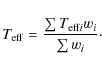
$\begin{displaymath}T_{\rm eff} = \frac{\sum {T_{{\rm eff} i}}{w_{i}} }{ \sum {w_{i}} } \cdot \end{displaymath}$

The weights in each line ratio is given as usually by ( $w_i = 1/\sigma_i^2.$ ), where $\sigma_i$ is the standard deviation computed in each line-ratio calibration (Table 2). This way we are giving more strength to the best calibrated line ratios.

4.2 Temperature uncertainties

The uncertainty on the final effective temperature is obtained after considering the standard deviation ( $\sigma$ ) of the effective temperatures given by each individual line ratio, and considering the number of line-ratios used to compute the weighted average:

$\begin{displaymath}\Delta T_{\rm eff} = \frac{\sigma}{\sqrt{N}} , \end{displaymath}$

where N is the number of independent ratios in the final selection of line ratios used to estimate the temperature.

Usually, the total number of line-ratios is used instead of only the independent ones. For multiple measurements of the same quantity, the uncertainties are derived by dividing the standard deviation by the square root of the number of independent measurements. However, all the line ratios are not independent of each other as some have spectral lines in common. Therefore we choose the number of independent line ratios by the chemical elements used in each ratio. Therefore we use a smaller number N that is the number of line ratios that we consider independent. To make this clear to the reader, let us consider an example where we used 3 different elements (Fe, V, Sc) and where we use 2 lines for each element. In this example we can built a total of 15 different line ratios. For these examples we consider the number of independent line ratios to be 3, which is given by the different combination of the elements (Fe-V, Fe-Sc, V-Sc). This is our point of view for estimating the uncertainties on the temperature; nevertheless the reader can choose a different approach to estimate the errors when using this calibration.

The typical error for the calibration will vary from $\sim$ 10-40 K, depending on the quality of the spectra and the spectral type of the stars. Solar twins will have the lower uncertainties, while the hotter and cooler stars will have the larger uncertainties, especially the cooler ones due to the increased difficulty in obtaining correct equivalent width measurements in the more crowded spectral range. We estimate that the systematic errors using this procedure is below 50 K.

4.3 Free code to estimate $T{_{\rm eff}}$

A free code was developed to use the procedure described above to estimate the effective temperature. The code was written in C++ and can be freely used in any machine as an extension to ARES, where ARES will automatically measure the EWs for the line list. It can be used to estimate the temperature. Depending on the computer speed and the type of stars, the process can derive a precise temperature in less than 1 min. For cooler stars it is slower because of the larger number of lines present in the spectra. This simple code and some quick instructions are available for download on the ARES web page: http://www.astro.up.pt/ sousasag/ares

5 Testing the calibration

5.1 Spectroscopic $T{_{\rm eff}}$ vs. line-ratio $T{_{\rm eff}}$ on the sample of calibration stars

The first test of the calibration was an inversion exercise where we used the sample of calibration stars to obtain the temperatures for the calibration stars. Figure 5 shows the comparison between the spectroscopic and the line-ratio effective temperatures. The figure shows excellent consistency except at the edges of the temperature range of the calibration stellar sample. This is caused by to the small number of stars in these regions when compared with the full sample (see Fig. 1). This occurs because the fitting function for each ratio is more precise for the middle region of the relations, while at the edges it is less precise in general. Nevertheless looking at Fig. 5 we can see that the consistency is excellent for the temperatures in the interval $\sim$ [4700-6100] K.

To fix the trend observed for the hotter stars, we performed a small correction for the stars with temperature higher than 6000 K. The correction was achieved by fitting a straight line to these stars (see Fig. 5), and we used this fit to ``push'' the offset stars closer to the identity line. The following condition equations are used to make this correction for the hotter stars:

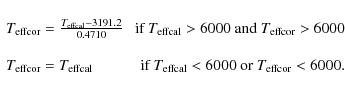
$\begin{displaymath}\begin{array}{lr} T_{\rm effcor}=\frac{T_{\rm effcal}-3191.2}... ... effcal} < 6000 \mbox{ or } T_{\rm effcor} < 6000 . \end{array}\end{displaymath}$

(1)

This correction is included in the code. For the cases where the correction is applied the code outputs both the corrected and the original values of the derived temperature. Figure 6 shows a clear improvement on the results for the calibration with a small correction. We now need to test this calibration on stars outside the calibration sample. This is done in the following sections.

We also show the error of the temperature calibration versus the stellar parameters in Fig. 7. From this figure we can see that the error dependence on the stellar parameters seems to be flat, indicating a clear independence with the stellar parameters. The dispersion of the error values seen in this figure should be a consequence of the error dependence on the S/N of the spectra.

5.2 The Sun via Ganymede

The more important test to our calibration is to use it on the Solar spectrum, estimate its temperature with the code, and compare it with the canonical solar temperature of 5777 K. Figure 4 shows this result. Using the process described previously, we determined an effective temperature for the Sun using an HARPS reflection spectra of the asteroid Ganymede. The result $5782 \pm 10$ K is perfectly consistent with the assumed canonical temperature of the Sun (5777 K).

$\begin{figure} \par\includegraphics[width=8cm,clip]{13388fg4.ps} \end{figure}$	Figure 4: Final result for the estimation of the effective temperature: case of the solar spectrum through the reflection of Ganymede.
Open with DEXTER

$\begin{figure} \par\includegraphics[width=8cm,clip]{13388fg5.ps} \end{figure}$	Figure 5: $T{_{\rm eff}}$ comparision within the sample. The offsets from the identity line at the edges come from the limits in $T{_{\rm eff}}$ of our sample of calibration stars.
Open with DEXTER

$\begin{figure} \par\includegraphics[width=8cm,clip]{13388fg6.ps} \end{figure}$	Figure 6: Same as Fig. 5 but considering the small correction for hotter stars following Eq. (1).
Open with DEXTER

$\begin{figure} \par\includegraphics[width=8cm,clip]{13388fg7.ps} \end{figure}$	Figure 7: Error of the temperature calibration versus stellar parameters.
Open with DEXTER

$\begin{figure} \par\includegraphics[width=8cm,clip]{13388fg8.ps} \end{figure}$	Figure 8: Comparison of the temperature derived from the line-ratio calibration vs. the spectroscopic temperature. This plot shows stars observed with 4 different spectrographs: HARPS, UVES, FEROS, and CORALIE. Note that the Harps stars in this plot do not belong to the calibration sample.
Open with DEXTER

5.3 HARPS, UVES, FEROS, and CORALIE spectra

We used our calibration and code for different stars outside the calibration sample and observed with different spectrographs. We used very high-resolution spectra ( $R \sim 110~000$ ) taken with HARPS and UVES and some mid-high resolution ( $R \sim 55~000$ ) data taken by FEROS and CORALIE. This test can verify that our line-ratio calibration also works on other spectra.

This sample is composed of 15 CORALIE spectra, 7 HARPS spectra, 44 UVES spectra, and 64 FEROS spectra. The spectroscopic effective temperature for these stars were obtained in Santos et al. (2005,2004) and Sousa et al. (2006). The equivalent widths for this spectra were obtained using ARES. For the CORALIE and HARPS spectra, the ``rejt'' parameter was varied according to the S/N of the spectra. For the UVES and FEROS spectra, we took a faster approach and used the same value of ``rejt'', 0.998 for the UVES spectrograph that have typical high S/N, and 0.990 for the FEROS spectra that have a typical lower value of S/N for this specific sample. Figure 8 shows the comparison between the spectroscopic temperature and the estimate using our line-ratio calibration. The result is very consistent (sigma $\sim$ 90 K) and shows that the calibration is valid for different spectrographs configurations and S/N.

Since in this case we fixed the value of ``rejt'' for FEROS and UVES spectra, we also tested the systematics of our calibration when using EWs computed with different values of ``rejt''. This is the same as studying the effects of systematically larger/smaller EWs on the temperatures derived from the line-ratio calibration.

$\begin{figure} \par\includegraphics[width=7.6cm,clip]{13388fg9.ps} \end{figure}$	Figure 9: Effective temperature determination using the calibration presented in this paper with different values of the ARES ``rejt'' parameter. Three different spectral types of stars with different S/N are shown. Top: Sun through Ganymede reflection; middle: HD 8326; bottom: HD 7449. See text for details.
Open with DEXTER

Table 3: Results of the calibration using different wavelength intervals.

5.4 Propagation of the uncertainties from ARES EWs measurements

To test how the calibration will react if we make a mistake in the continuum position for the EW measurements, we used different values for the ARES parameter ``rejt''. This will put the continuum position systematically higher or lower depending on the S/N of the spectra. Figure 9 shows the variation of the effective temperature for different values of ``rejt'', and for 3 different types of stars, the Sun, a cooler, and a hotter star. The variation in temperature is expected because, when we modify the continuum position (changing the ``rejt'' value) we are affecting the EW measurements. Since the weaker lines are affected more than the stronger lines, we will have an offset in the value of the line ratios producing a systematic shift on the derived effective temperature for all line ratios. In Fig. 9 we can see that the variation in effective temperature does not change by more than 40-50 K in the worse cases imaginable. This result is very significant, and it means that, even when using different subjective measurements of the EWs, the final result for the temperature for a given star will not change by more than the 40-50 K, i.e. within the expected errors.

5.5 Smaller wavelength intervals

The final test was to see how the calibration would react to the use of lines in different wavelength intervals. This can be useful if interested in using this calibration on data that have a specific and/or a smaller wavelength coverage. To test this situation on different effective temperatures, we used the same 3 spectra as in Sect. 5.4: the Sun, a cooler star, and a hotter star. For these 3 examples we defined 3 shorter wavelength intervals: [4500 Å-5500 Å], [5000 Å-6000 Å], and [6000 Å-7000 Å] and tested the calibration for the lines in these intervals. The results are presented in Table 3, which shows that the calibration works consistently on different wavelength intervals.

6 Conclusions

We have presented a fast and automatic procedure for deriving precise effective temperatures for solar-type stars. We selected 433 line-ratios that were calibrated using a large sample composed of 451 FGK dwarf stars. These line ratios can be used to derive the effective temperatures with high precision using a totally automatic and fast procedure. For this purpose, we built a simple code available as an extension to ARES. The calibration was tested by considering different spectrographs, and the results are consistent with the temperatures that we find using a detailed spectroscopic analysis. Moreover, we tested how this calibration would react to the subjectivity of ARES EWs measurements and concluded that the variation in the estimated temperature is not greater than $\sim$ 40 K. Finally, we presented the use of this calibration using shorter wavelength intervals and demonstrated that the temperature estimations are consistent.

Acknowledgements

S.G.S would like to acknowledge the support from the Fundação para a Ciência e Tecnologia (Portugal) in the form of grant SFRH/BPD/47611/2008. A.A. would like to acknowledge useful input on this project from Alexandra Ecuvillon and Suzanne Aigrain. NCS would like to acknowledge the support by the European Research Council/European Community under the FP7 through a Starting Grant, as well as the support from the Fundação para a Ciência e a Tecnologia (FCT), Portugal, through program Ciência 2007. We would also like to acknowledge support from the FCT in the form of grants PTDC/CTE-AST/098528/2008, PTDC/CTE-AST/098604/2008, and PTDC/CTE-AST/66181/2006. This research was also supported by the Spanish Ministry of Science and Innovation (MICINN).

References

Gray, D. F. 1994, PASP, 106, 1248 [NASA ADS] [CrossRef] [Google Scholar]
Gray, D. F. 2004, Adv. Space Res., 34, 308 [NASA ADS] [CrossRef] [Google Scholar]
Gray, D. F., & Brown, K. 2001, PASP, 113, 723 [NASA ADS] [CrossRef] [Google Scholar]
Gray, D. F., & Johanson, H. L. 1991, PASP, 103, 439 [NASA ADS] [CrossRef] [Google Scholar]
Kovtyukh, V. V., Soubiran, C., Belik, S. I., & Gorlova, N. I. 2003, A&A, 411, 559 [NASA ADS] [CrossRef] [EDP Sciences] [Google Scholar]
Neves, V., Santos, N. C., Sousa, S. G., Correia, A. C. M., & Israelian, G. 2009, A&A, 497, 563 [NASA ADS] [CrossRef] [EDP Sciences] [Google Scholar]
Nordström, B., Mayor, M., Andersen, J., et al. 2004, A&A, 418, 989 [NASA ADS] [CrossRef] [EDP Sciences] [Google Scholar]
Santos, N. C., Israelian, G., & Mayor, M. 2004, A&A, 415, 1153 [NASA ADS] [CrossRef] [EDP Sciences] [Google Scholar]
Santos, N. C., Israelian, G., Mayor, M., et al. 2005, A&A, 437, 1127 [NASA ADS] [CrossRef] [EDP Sciences] [Google Scholar]
Sousa, S. G., Santos, N. C., Israelian, G., Mayor, M., & Monteiro, M. J. P. F. G. 2006, A&A, 458, 873 [NASA ADS] [CrossRef] [EDP Sciences] [Google Scholar]
Sousa, S. G., Santos, N. C., Israelian, G., Mayor, M., & Monteiro, M. J. P. F. G. 2007, A&A, 469, 783 [NASA ADS] [CrossRef] [EDP Sciences] [Google Scholar]
Sousa, S. G., Santos, N. C., Mayor, M., et al. 2008, A&A, 487, 373 [NASA ADS] [CrossRef] [EDP Sciences] [MathSciNet] [Google Scholar]
Strassmeier, K. G., & Schordan, P. 2000, Astron. Nachr., 321, 277 [NASA ADS] [CrossRef] [Google Scholar]

Footnotes

... ratios: Full Table 2 and line list are only available in electronic form at the CDS via anonymous ftp to cdsarc.u-strasbg.fr (130.79.128.5) or via http://cdsweb.u-strasbg.fr/cgi-bin/qcat?J/A+A/512/A13
... analyze: http://www.astro.up.pt/ sousasag/ares

All Tables

Table 1: Spectral lines added to the lists of lines presented in Sousa et al. (2008) and in Neves et al. (2009).

Table 2: Effective temperature vs. line-ratio calibration table.

Table 3: Results of the calibration using different wavelength intervals.

All Figures

$\begin{figure} \par\includegraphics[width=8cm,clip]{13388fg1.ps} \end{figure}$	Figure 1: Effective temperature distribution of the calibration sample.
Open with DEXTER
In the text

$\begin{figure} \par\includegraphics[width=8cm,clip]{13388fg2.ps} \end{figure}$	Figure 2: Progress in the calibration of the ratio composed of the lines: SiI(6142.49 Å) and TiI(6126.22 Å). The dashed lines represent the 2 sigma from each fit. The open circles represent the points that were removal in the process. The final points and respective calibration are plotted at the bottom.
Open with DEXTER
In the text

$\begin{figure} \par\includegraphics[width=17.4cm,clip]{13388fg3.ps} \end{figure}$	Figure 3: Evaluation of the different fits for 3 different line ratios (r) ( from top to bottom - line ratios 456, 651 and 917). In the left panels we plot `` $T{_{\rm eff}}$ vs. r'', In the middle we plot `` $T{_{\rm eff}}$ vs. 1/r''. In the right panels we plot `` $T{_{\rm eff}}$ vs. $\log(r)$ ''. The dashed line represents the final linear fit, and the filled line represents the 3rd order polynomial fit.
Open with DEXTER
In the text

$\begin{figure} \par\includegraphics[width=8cm,clip]{13388fg4.ps} \end{figure}$	Figure 4: Final result for the estimation of the effective temperature: case of the solar spectrum through the reflection of Ganymede.
Open with DEXTER
In the text

$\begin{figure} \par\includegraphics[width=8cm,clip]{13388fg5.ps} \end{figure}$	Figure 5: $T{_{\rm eff}}$ comparision within the sample. The offsets from the identity line at the edges come from the limits in $T{_{\rm eff}}$ of our sample of calibration stars.
Open with DEXTER
In the text

$\begin{figure} \par\includegraphics[width=8cm,clip]{13388fg6.ps} \end{figure}$	Figure 6: Same as Fig. 5 but considering the small correction for hotter stars following Eq. (1).
Open with DEXTER
In the text

$\begin{figure} \par\includegraphics[width=8cm,clip]{13388fg7.ps} \end{figure}$	Figure 7: Error of the temperature calibration versus stellar parameters.
Open with DEXTER
In the text

$\begin{figure} \par\includegraphics[width=8cm,clip]{13388fg8.ps} \end{figure}$	Figure 8: Comparison of the temperature derived from the line-ratio calibration vs. the spectroscopic temperature. This plot shows stars observed with 4 different spectrographs: HARPS, UVES, FEROS, and CORALIE. Note that the Harps stars in this plot do not belong to the calibration sample.
Open with DEXTER
In the text

$\begin{figure} \par\includegraphics[width=7.6cm,clip]{13388fg9.ps} \end{figure}$	Figure 9: Effective temperature determination using the calibration presented in this paper with different values of the ARES ``rejt'' parameter. Three different spectral types of stars with different S/N are shown. Top: Sun through Ganymede reflection; middle: HD 8326; bottom: HD 7449. See text for details.
Open with DEXTER
In the text

Current usage metrics show cumulative count of Article Views (full-text article views including HTML views, PDF and ePub downloads, according to the available data) and Abstracts Views on Vision4Press platform.

Data correspond to usage on the plateform after 2015. The current usage metrics is available 48-96 hours after online publication and is updated daily on week days.

Initial download of the metrics may take a while.