A&A 512, A67 (2010)

2MASS wide field extinction maps

III. The Taurus, Perseus, and California cloud complexes

M. Lombardi^1,2 - C. J. Lada³ - J. Alves⁴

1 - European Southern Observatory, Karl-Schwarzschild-Straße 2, 85748 Garching bei München, Germany
2 - University of Milan, Department of Physics, via Celoria 16, 20133 Milan, Italy (on leave)
3 - Harvard-Smithsonian Center for Astrophysics, Mail Stop 72, 60 Garden Street, Cambridge, MA 02138, UK
4 - Calar Alto Observatory - Centro Astronómico Hispano Alemán, C/Jesús Durbán Remón 2-2, 04004 Almeria, Spain

Received 9 June 2009 / Accepted 20 October 2009

Abstract
We present a near-infrared extinction map of a large region in the sky (3500 deg²) in the general directions of Taurus, Perseus, and Aries. The map has been obtained using robust and optimal methods to map dust column density at near-infrared wavelengths (N ICER, described in Lombardi & Alves 2001, A&A, 377, 1023 and N ICEST, described in Lombardi 2009, A&A, 493, 735) toward 23 million stars from the Two Micron All Sky Survey (2MASS) point source catalog. We measure extinction as low as with a 1- significance, and a resolution of in our map. A section of our map encompasses the Taurus, Perseus, and California molecular cloud complexes. We determine the distances of the clouds by comparing the observed density of foreground stars with the prediction of galactic models, and we obtain results that are in excellent agreement with recent VLBI parallax measurements. We characterize the large-scale structure of the map and find a region close to the galactic plane ( , ) with small extinction ( ); we name this region the Perseus-Andromeda hole. We find that over the region that encompasses the Taurus, Perseus, and California clouds the column density measurements below are perfectly described by a log-normal distribution, and that a significant deviation is observed at larger extinction values. If turbulence models are invoked to justify the log-normal distribution, the observed departure could be interpreted as the result of the effect of gravity that acts on the cores of the clouds. Finally, we investigate the cloud structure function, and show that significant deviations from the results predicted by turbulent models are observed in at least one cloud.

Key words: ISM: clouds - dust, extinction - ISM: individual objects: Taurus molecular complex - ISM: structure - methods: statistical

1 Introduction

This paper is the third of a series where we apply an optimized multi-band technique dubbed Near-Infrared Color Excess Revisited (N ICER Lombardi & Alves 2001, hereafter Paper 0) to study the structure of nearby molecular dark clouds using the Two Micron All Sky Survey (2MASS; Kleinmann et al. 1994). Previously, we considered the Pipe nebula (see Lombardi et al. 2006, hereafter Paper I) and the Ophiuchus and Lupus complexes (Lombardi et al. 2008, hereafter Paper II). In this paper we present a wide field extinction map, constructed from 23 million JHK 2MASS photometric measurements, of a large region covering , and including the Taurus, Perseus, and California complexes, as well as the high-galactic latitude clouds MBM 8, MBM 12, and MBM 16 and the M 31 and M 33 galaxies.

The main aim of our coordinated study of nearby molecular clouds is to investigate in detail the large-scale structure of these clouds, down to the lowest column densities measurable with this technique, which are below the column density threshold required for the detection of the CO molecule (e.g. Lombardi et al. 2006; Alves et al. 1999). In addition, the use of an uniform dataset and of a consistent and well tested pipeline allows us to characterize many properties of molecular clouds and to identify cloud-to-cloud variations in such properties.

The advantages of using near-infrared dust extinction as a column density tracer have been discussed elsewhere (Alves et al. 2001; Lombardi et al. 2006; Lada et al. 1994; Alves et al. 1999). Indeed, Goodman et al. (2008) used data from the COMPLETE survey (Ridge et al. 2006) to assess and compare three methods for measuring column density in molecular clouds, namely, near-infrared extinction (N ICER), thermal emission in the far-IR (IRAS), and CO line emission. They found that observations of dust are a better column density tracer than observations of molecular gas (CO), and that observations of dust extinction in particular provide more robust measurements of column density than observations of dust emission, mainly because of the dependence of the latter measurements on uncertain knowledge of dust temperatures and emissivities.

This paper is the first to use, in some key analyses, the improved N ICEST method (Lombardi 2009), which copes well with the sub-pixel inhomogeneities present in the high-column density regions of the maps. The inhomogeneities can either be due to steep gradients in the column density map, to the effect of turbulent fragmentation, or to the increased presence of foreground stars, and they bias the measurements towards lower column densities. All these effects are expected to be most severe in the densest regions of dark complexes, i.e. in very limited parts of the large areas considered in this paper. Nevertheless, because of the relevance of these regions in the process of star formation, it is important to understand this bias and to correct for it.

Taurus is one of the best studied molecular cloud complexes in the Galaxy. It has about 200 young low-mass stars and it is one of the Rosetta stones of star formation research with the identification, about 60 years ago, of irregular, emission-line variable (T-Tauri) stars physically associated with the cloud (Joy 1945) and the subsequent recognition of their extreme youth (Herbig 1962). Taurus is also the prototype low-mass, distributed star forming region where stars appear to form in relative isolation compared to the more common embedded cluster mode of formation that characterizes regions such as Orion and Perseus. The Taurus cloud complex has also been the prototype for molecular-line studies of dense proto-stellar and pre-stellar cores (e.g. Myers et al. 1979). Most recently, a 100 deg² survey of the Taurus molecular cloud region in ¹²CO and ¹³CO J=1-0 and with at a resolution of and respectively was presented in Narayanan et al. (2008) and Goldsmith et al. (2008). There have also been extensive dust extinction studies done of the Taurus dark clouds (Cernicharo & Guelin 1987; Dobashi et al. 2005; Cernicharo et al. 1985; Cernicharo & Bachiller 1984; Meistas & Straizys 1981; Straizys & Meistas 1980; Cambrésy 1999) using either star counts or color-excesses. The current best estimate of the distance to the Taurus complex, using VLBI, is (Loinard et al. 2007). These authors also found that the thickness of the complex is comparable to its extent, or about .

Like Taurus, Perseus is a well known star forming region. It is the prototype intermediate mass star forming region, with young B-stars and two clusters, IC 348 (Muench et al. 2007) and NGC 1333 (Lada et al. 1996). The complex seems to be associated with the Perseus OB2 association (de Zeeuw et al. 1999) at a distance of about 250 pc (Bally 2008).

The California molecular cloud is not as well known as Taurus and Perseus. Only recently, and as a by-product of the analysis presented in this paper, it has been recognized as a major cloud complex and studied in detail by Lada et al. (2009). In that paper we estimated the distance of this massive giant molecular complex to be , and stressed that this cloud is surprisingly similar in mass, distance, and shape to the much better studied Orion molecular cloud; interestingly, however, the California cloud displays much less star formation.

The area considered in this paper also includes the two spiral galaxies M 31 and M 33, and a few high galactic latitude clouds (MBM 8, MBM 12, and MBM 16). However, the limited angular resolution achievable using the 2MASS archive does not allow to study in detail the properties of these clouds, and therefore here we focus our efforts to the three main clouds mentioned above.

This paper is organized as follows. In Sect. 2 we briefly describe the technique used to map the dust and we present the main results obtained. A statistical analysis of our results and a discussion of the bias introduced by foreground stars and unresolved substructures is presented in Sect. 3. Section 4 is devoted to the mass estimate of the cloud complexes. The structure functions and the scaling index ratio of the three clouds are presented and discussed in Sect. 5. Finally, we summarize the results obtained in this paper in Sect. 6.

2 N ICER and N ICEST extinction maps

We carried out the data analysis using the N ICER and N ICEST methods described in Paper 0 and in Lombardi (2009). Near infrared J (1.25 m), H (1.65 m), and band (2.17 m) magnitudes of stars in a large region of the sky which includes the dark clouds were taken from the Two Micron All Sky Survey (2MASS; Kleinmann et al. 1994). In particular, we selected all 2MASS reliable point sources within the boundaries

Our selection criteria excluded sources that are likely to be contaminated by extended objects ( ) and sources associated with minor planets ( ); in addition, for the selected sources we retained only the bands with good photometry ( ). The chosen area is 3500 square degrees and contains approximately 23 million point sources from the 2MASS catalog. Note that since the region spans several degrees in galactic latitude, the local density of background stars changes significantly in the field; as a result, since we used a fixed size for the smoothing of the extinction map (see below), the noise of the map increases as b increases.

We then generated a preliminary extinction map which, as described in Paper 0, was mainly used as a first check of the parameters adopted, to select a control region on the field, and to obtain the photometric parameters to be used in the final map. We identified a large region that is apparently affected by only a negligible extinction (see below), and used the colors of stars in this control field as reference ones.

Using the information provided by the control field, we generated a second map, which is thus ``calibrated'' (i.e., provides already, for each position in our field, a reliable estimate of the column density). In this step we used the Indebetouw et al. (2005) 2MASS reddening law. Similar to Paper I, we then considered the color-color diagram for the stars in the catalog to check for possible signs of anomalous star colors. The result, presented in Fig. 1, shows two trails of stars parallel to the reddening vector for .

As discussed in detail in Paper I, the bifurcation is likely to be due to Asymptotic Giant Branch (AGB) stars. We verified this assumption by considering the spatial distribution of two subsets of stars defined in the color-color diagram as

Figure 2 shows the results obtained and proves that as expected, sample A is associated with the densest regions of the molecular cloud, while sample B is distributed on the whole field with a strong preference for low galactic latitude regions. We also considered in Fig. 3 the two histograms of the K-band magnitude distribution for the two samples. As expected, sample Ashows a broad distribution, which can be essentially described as a simple power-law luminosity function up to ; note that the completeness limit of our sample is significantly brighter than the typical 2MASS completeness in the K band ( at completeness) because of the stricter selection employed here (small photometric errors in all bands) and because most sample A stars come from low galactic latitude regions (where the increased density of stars significantly reduces the completeness of the 2MASS). Sample B stars show a bimodal distribution, with a broad peak at . A possibility is that we are looking at the same population of Asymptotic Giant Branch (AGB) stars identified in Paper II, but spread at different distances because of the higher galactic latitudes considered here.

Following Paper II, we then investigated the extinction-corrected color-color diagram (see Fig. 4), obtained by estimating, for each star, its ``intrinsic'' colors, i.e. the extinction corrected colors from the extinction at the star's location as provided by the N ICER map. In other words, we computed for each star

where is the N ICER estimated extinction in the direction of the star from the angularly close objects, as given by Eq. (7) below. A comparison of Fig. 4 with Fig. 1 shows that the many stars in upper branch, sample A, are moved toward the peak of the density in the lower-left part of the plot, while the lower branch, sample B, is largely unaffected, a result in agreement with Fig. 2. Note that the residual stars appearing in the upper branch are likely to be the effect of an inaccurate extinction correction due to small-scale inhomogeneities not captured by our analysis; similarly, the tail at negative colors is due to ``over-corrected'' stars (for example foreground stars observed in projection to a cloud). In any case, Fig. 2 shows that the number of contaminating AGB stars is negligible, and that no noticeable effects are expected in the 2MASS extinction map. For this reason, we decided not to correct for this contamination and to use the whole 2MASS input catalog for the analysis (in contrast, we proceeded with a correction in Paper II because of the much more pronounced contamination).

Figure 5 shows the final 2MASS/N ICER extinction map of the whole region considered here. We recall that in N ICER the final map can be generated using different smoothing techniques (see Lombardi 2002, for a discussion on the characteristics and merits of various interpolators). As pointed out in Paper 0, generally these techniques produce comparable results, and thus we focused here on the simple moving weight average:

where is the extinction at the angular position , is the extinction of the nth star, and is the weight for the nth star for the pixel at the location :

Hence, the weight for the nth star is composed by two factors: (i) , i.e. a function of the angular distance between the star and the point where the extinction has to be interpolated, and (ii) , the inverse of the inferred variance on the estimate of A_K from the star. The first factor, parametrized by the weight function W, was taken here to be a Gaussian.

The map of Fig. 5 was generated on a grid of approximately  points, with scale per pixel, and with Gaussian smoothing characterized by . Note that in the weighted average of Eq. (7) we also introduced an iterative -clipping at 3- error (see Paper 0). The average, effective density of stars is 2.8 stars per pixel, but as noted above this value changes significantly with galactic latitude; this density guarantees an average (1-) error on A_K of 0.04 mag in the marked box of Fig. 5.

We also constructed a N ICEST extinction map (not shown here, but used in some of the results presented below), obtained by using the modified estimator (Lombardi 2009)

where the modified weight is a combination of the original weight used in N ICER, of the slope of the number counts in the Hband, and of the extinction coefficient in the H band (see Indebetouw et al. 2005). The N ICEST map is visually identical to the N ICER map, but is more appropriate for a study of the high column-density regions.

The largest extinction was measured close to L1495, where  mag for N ICER and  mag for N ICEST. The expected error on the extinction A_K was evaluated from the relation (see Paper 0)

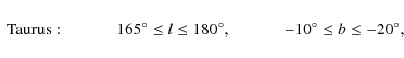
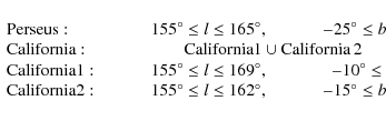
As expected, we observe a significant gradient along the galactic latitude. Other variations in the expected errors can be associated with bright stars, galaxies, and the cloud itself (dark areas). Because of the relatively large variations on the noise of the extinction map, clearly a detailed analysis of Fig. 5 should be carried out using in addition the noise map. Figure 6 shows in greater detail the absorption maps we obtain for the Taurus, Perseus, and California complexes, and allows us to appreciate better the details that we can obtain by applying the N ICER method to the good quality 2MASS data. In this figure we also displayed the boundaries that we use throughout this paper and that we assign to the three clouds considered in this paper. In particular, we define

We show in Fig. 7 a very low resolution extinction map of the whole field. By averaging the extinction with a Gaussian kernel at resolution, we effectively make use of thousands stars per map element, and thus decrease to a negligible level the statistical error associated to the intrinsic scatter of star colors or to the photometric errors. Because of its very-high sensitivity, this map is able to reveal diffuse, low extinctions extending on several degrees in the sky. Note, in particular, the presence of an region (with peaks up to ) at and , and a large area at and with very small values of extinction. This latter region, that we name ``Perseus-Andromeda hole'', extends to very low galactic latitudes, up to , and has a minimum extinction around and . The hole also appears to coincide with the center of a ring of high-galactic latitude clouds the ``hole'' is also visible in CO maps (Magnani et al. 2000; Bhatt 2000). The simple fact that we measure a negative extinction over a relatively large area indicates that our map is affected by a small bias (a constant offset), that can be attributed to the presence of a residual extinction in the control field. An analysis on the overall distribution of column density measurements for the area shown in Fig. 6 (see below Sect. 3.3) confirms that we are under-estimating the extinction by at least in A_K. In reality, it is unlikely that our bias is much larger than this value for several reasons:

• the area studied in this paper is very large, , and extends from the galactic plane to high galactic latitudes. Therefore it is very likely that at least in some region of our map the extinction is negligible;
• the DSS-based Dobashi et al. (2005) maps show low extinction at the location of the ``hole'';
• the IRAS measurements for the region that occupies the Perseus-Andromeda hole have been translated from Schlegel et al. (1998) into a visual extinction , corresponding to ; a similar extinction can be derived from the IRIS map (Miville-Deschênes & Lagache 2005). If these values are taken, our overall bias would be . This is of course possible, but note also that possible systematic uncertainties present in these IRAS estimates, and in particular the uncertainties inherent to the DIRBE calibration and to the zodiacal model, are likely to be of the order of one tenth of a visual magnitude, i.e. comparable to the detection itself.

In summary, we expect that in the Perseus-Andromeda hole the column density is very small, almost certainly . This large low column density region, together with a smaller one at and , could help us to investigate the structure and internal geometry of the Milky Way, and could also be of interest for extragalactic studies. In any case, we stress that the extinction measurements performed using color-excess techniques are not only relative (because, clearly, we have to select a control-field where the fiducial extinction is taken to be zero), but they can probe the extinction only up to the typical distance of the stars in the catalog (which, especially for regions close to the galactic plane, might be closer than the distance of some ``background'' clouds).

Finally, the low statistical uncertainty expected for the map of Fig. 7 can be used to check the presence of systematic errors. In this respect, the only significant anomaly we could detect is a general pattern that extends along lines of equal right ascension, and that is visible as stripes in the lower part of Fig. 7 (see also Fig. 5). This pattern is a known systematic effect of the 2MASS point source catalog, and is directly related to the observing strategy used (which is based on tiles aligned with the equatorial coordinates, further split in  images). This problem is most likely due to errors on the determination of the zero-points for the various observation stripes, or to other effects induced by the different observational conditions (and, in some cases, also to data reduction issues present in high density regions; see Paper I).

3 Statistical analysis

3.1 Reddening law

The use of two different colors, J-H and H-K, allows us to verify that the reddening law used throughout this paper is consistent with the data. For this purpose, we partitioned all stars with complete, reliable measurements in all bands, into different bins corresponding to the individual original measurements (we used a bin size of ). Then, we evaluated the average NIR colors in each group of stars in the same bin and the corresponding statistical uncertainties (estimated from on the photometry errors of the 2MASS catalog). The results obtained are shown in Fig. 8 together with the normal infrared reddening law in the 2MASS photometric system (Indebetouw et al. 2005). This plot shows that there are no significant deviations from the normal reddening law over the whole range of extinctions and directions investigated here.

3.2 Foreground star contamination and cloud distance

Foreground stars observed in projection on a dark cloud do not carry any information on the cloud column density, and thus they dilute the signal and add noise. Both effects are proportional to the fraction f of foreground stars, and it is thus important to verify that fis sufficiently small. For nearby molecular clouds, f is usually very small and negligible on the outskirts of the clouds (typical values are ), but increases significantly on the very dense regions, where the density of observed background stars decreases dramatically. In addition, many dense cores host young stellar objects: these stars, if moderately embedded, show only a fraction of the true, total column density of the cloud. As a result, the extinction in the direction of dense regions can be severely underestimated.

Table 1:   The average value of foreground stars found in the various complexes.

In order to evaluate quantitatively the fraction f of foreground stars we selected high-extinction regions characterized by . We then flagged all stars in these regions that show ``no'' extinction, i.e. stars with column densities less than 3- above the background, compatible with no or negligible extinctions. We performed these tests for the whole area shown in Fig. 6, and calculated the local density of foreground stars by taking into account the area in the sky occupied by regions with . Figure 9 shows the local density of foreground stars, averaged over connected regions of high extinction. For Perseus, we measure an anomalous density of foreground stars around the reflection nebula NGC 1333, which is known to contain several embedded young stellar objects (YSOs). It is evident that the each of the three regions shows a rather uniform density, a strong indication that the clouds are connected structures at about the same distance. A possible exception is the Perseus cloud, which seems to show rather large differences in Fig. 9. Therefore, we performed a detailed analysis by dividing the Perseus region into three areas: one, to the North, that includes B3, B4, and B5; one, to the South, that includes B1, L1455, and L1448; and a third, which includes NGC 1333, and is only considered to isolate the effects of the YSO cluster from the estimate of the density of foreground stars.

A visual inspection of Fig. 9 also shows that California has a significantly higher density of foreground stars, suggesting that this cloud is located at a significantly higher distance than the other two complexes (see Lada et al. 2009). The results of a more quantitative analysis are presented in the Table 1, were we also report the cloud distances evaluated by comparing the observed densities with the values inferred from the Galactic model by Robin et al. (2003) at different distances (see Fig. 10).

As shown by the second and third line from the bottom of this table, the Northern regions of the Perseus cloud has an average density of foreground stars of that appears to be significantly larger than the one found in the Southern regions. In order to better quantify this result, we note that from simple error propagation the difference between the two densities is , which is consistent with zero only at 1.8-. In other words, the data seem to suggest a genuine, although relatively small, difference between the distances of the Northern and Southern regions of the Perseus cloud. We also note the extent covered by this cloud in the sky, approximately , corresponds to approximately , at the cloud distance, a value smaller but comparable to the measured distance difference. In summary, even if the distance difference is real (a claim that we cannot make here), the various regions could still be physically connected if the Perseus complex is extending along the line of sight.

The agreement between the distances estimated for the Perseus and Taurus clouds and the results known from the literature is amazing and shows that the Galactic model used here (Robin et al. 2003) is extremely accurate and reliable. For example, the Perseus distance is in excellent agreement with recent multi-epoch VLBI maser observations of the YSO SVS 13 in NGC 1333 (Hirota et al. 2008), which provide . Similarly, the Taurus distance is in excellent agreement with a VLBI determination, (Loinard et al. 2007).

Finally, we note that the accuracy and reliability of the distances based on the density of foreground stars suggests that we can use this technique for clouds for which no VLBI distance is available (such as the California cloud) or possible (for example because of the lack of maser sources or of the large distance of the clouds). A further advantage of the technique used in this paper is that its accuracy is mainly driven by the number of foreground stars, a quantity that for equally-sized clouds is almost independent of the cloud distance. Indeed, the density of foreground stars increases quadratically (at least up to distances of a few kpc, cf. Fig. 10) with the distance of the cloud, while the area covered by the cloud decreases quadratically, thus leaving their product, the number of foreground stars, unchanged.

3.3 Column density probability distribution

The probability distribution for the volume density in molecular clouds is expected to be log-normal for isothermal, turbulent flows (e.g. Passot & Vázquez-Semadeni 1998; Scalo et al. 1998; Padoan et al. 1997b; Vazquez-Semadeni 1994). Under certain assumptions, verified in relatively ``thin'' molecular clouds, the probability distribution for the column density, i.e. the volume density integrated along the line of sight, is also expected to follow a log-normal distribution (Vázquez-Semadeni & García 2001).

Figure 11 reports the probability distributions of column densities for the Taurus, Perseus, and California region, i.e. the relative probability of column density measurements for each pixel of Fig. 6. This probability is thus calculated for the N ICER map, but we stress that no differences would be observed for a N ICEST map up to (which, as noted above, only differ from the N ICER map in the high column density regions). We fitted the column density histograms with log-normal distributions of the form

convolved with a Gaussian kernel characterized by a standard deviation to take into account the expected statistical error on the column density measurements. We obtained an extremely good fit on the whole region mapped in Fig. 6. The best-fit parameters, and their errors, are shown in Table 2. The error analysis has been carried out using a Markov chain Monte Carlo (MCMC) sampler of the posterior probability distribution for the fitting parameters. The full distribution and covariances observed in the four fitting parameters are shown in Fig. 12; the uncertainties reported in Table 2 are derived from the MCMC sampler.

Two features of Fig. 11 are evident. First, we note that there is a significant number of column density estimates with negative values. These can only partially be attributed to the broadening due to the uncertainties on the column density measurement, which are expected to be of the order of . Rather, this analysis, which we stress is based solely in the area shown in Fig. 6, suggests again that our extinction values are slightly under-estimated. If one believes, from theoretical or observational grounds, that the log-normal distribution is a good fit to the column density measurements, than the amount of this bias is provided by the fit parameter A₀, because this is the quantity directly responsible for a pure shift in the column density in Eq. (11). If we follow this path, then we can estimate the bias in the extinction values reported in our map to be . This value agrees well with our previous results on the Perseus-Andromeda hole: it is smaller than , as it should be (because we actually detect a extinction in the hole) and it actually would predict a extinction in the hole, which is very close to the IRAS measurements (see above Sect. 2).

A second feature visible in Fig. 11 is the excess of flux at the higher column densities, approximately for . We tentatively interpret this as the signature of relatively dense cores, where the original assumptions of a turbulent flow are likely to break down (e.g. Lada et al. 2008; Barranco & Goodman 1998). In particular, the clear break at suggests that gravity might start playing a dominant role for these relatively dense structures, and that for the even higher column densities the effects of turbulence might be almost completely canceled by the large gravitational fields.

Table 2:   The best-fit parameters and their 1- errors for the log-normal distribution used to fit the column density probability shown in Fig. 11 (see Eq. (11) for the meaning of the various quantities).

3.4 Small-scale inhomogeneities

Sub-pixel inhomogeneities play an important role in extinction maps of molecular clouds, especially at the resolution achievable from the 2MASS data. Lada et al. (1994) first recognized that the local dispersion of extinction measurements increases with the column density: in a small patch of the sky, the scatter of the individual star column density estimates is proportional to the average local column density estimate. The observed scatter in the column density is mainly due to the photometric errors, to the intrinsic scatter in the NIR star colors, and to the effect of unresolved structure on scales smaller than the resolution of the smoothed maps. The latter effect could be due to either small-scale random inhomogeneities in the cloud projected density or unresolved but otherwise systematic density gradients. The presence of any random inhomogeneities is important because they might contain signatures of turbulent motions (see, e.g. Padoan et al. 1997a; Miesch & Bally 1994), and because they are bound to bias the extinction measurements in high-column density regions (and, especially, in the very dense cores; see Lombardi 2009).

In order to better quantify the effect of unresolved structure on small scales, consider the quantity (cf. Paper II)

This quantity estimates the observed scatter in column densities which, as mentioned above, also includes the effects of photometric errors and intrinsic scatter of star colors. As shown in Paper II, one can instead use a different estimator, the , defined as

where the definitions of Eqs. (8), (10), and (12) have been used. In Paper II we showed that the is expected to provide information on the small-scale structure of the cloud, and in particular that the following relation holds:

where represents the difference between the true extinction at the position of the nth star, and of the local extinction measurement provided by Eq. (7) (and thus smoothed by the window function W). The interpretation of  as a ``variance'' of small scale structures is thus evident.

We evaluated the map for the whole field and identified regions with large small-scale inhomogeneities. The results, shown in Fig. 13, confirm our expectations: inhomogeneities are mostly present in high column density regions, while at low extinctions (approximately below ) substructures are either on scales large enough to be detected at our resolution ( ), or are negligible.

Figure 14 shows the average as a function of the local extinction A_K for the map in Fig. 5. If we compare the dashed line, representing the average value of in bins of in A_K, with the average variance on the estimate of from a single star, which is approximately , we can see that local inhomogeneities start to be the prevalent source of errors in extinction maps for .

As for the Papers I and II, we note here that a complete characterization of the properties of inhomogeneities cannot be performed using the results shown in Fig. 14 alone. However, this plot can be used very efficiently to validate specific models for inhomogeneities. For example, the contamination from foreground stars shows up in the A_K- diagram as separate trails with parabolic shapes that divert from the main locus of points.

4 Mass estimate

Table 3:   The masses of the Taurus, Perseus, and California dark complexes.

The cloud mass M can be derived from the A_K extinction map using the following simple relation

where d is the cloud distance, is the mean molecular weight corrected for the helium abundance, is the ratio (Savage & Mathis 1979; see also Bohlin et al. 1978; Lilley 1955), and the integral is evaluated over the whole field . Assuming a standard cloud composition (hydrogen, helium, and  dust), we find and the total masses reported in Table 3. These masses are calculated for the indicated distances, and should be rescaled appropriately for different distances.

Figure 15 shows the relationship between the integrated mass distribution and the extinction in A_K, calculated using the N ICEST technique. Note that regions with extinction larger than account for in Taurus, for in Perseus, and for less than  for in California. Hence, we do not expect any significant underestimation in the cloud mass due to unresolved dense cores. Note that the apparent difference between the curve presented in Fig. 15 and in Fig. 4 of Lada et al. (2009) is due to the different resolution of the extinction maps used to produce the cumulative mass fraction plots.

Although Fig. 15 is valuable to understand the distribution of column densities and its impact on the mass estimates of the various clouds, it is not particularly useful to make comparisons on the physical properties of the various clouds. Indeed, the measured cloud cumulative mass distribution depends on the resolution of the map used to compute it (a low resolution map will be unable to trace the high density peaks, and will produce a cumulative mass distribution truncated at large column densities). In addition, other factors such as the density of background stars available for the extinction map and the contamination by foreground stars play a role in the final measured cumulative mass distribution. Hence, in order to be able to make a comparison among the various clouds, we made an effort to produce maps that probe, as much as possible, the various clouds under the same physical conditions. In particular, we imposed the following constraints:

1.

the physical resolution of the various maps is identical, so that we probe the same physical scales. In practice, this forces us to degrade the angular resolutions of the maps of the nearby clouds to match the physical resolution of the most distant complex (California in our case). We perform this step by using, for each cloud, a pixel scale proportional to the inverse of its estimated distance;

2.

all maps have, on average, the same density of stars per pixel, so that the noise properties of the various maps are comparable. In order to reach this goal, we discard a fraction of stars in the clouds that have a large density of background stars per pixel;

3.

the expected number of foreground stars per pixel is identical for all clouds. We ensure this by adding in the star catalogs of the various clouds an appropriate number of artificial foreground stars, with colors randomly chosen from the observed color distribution of sources in the control field. Note that in this process we make use of the estimated density of foreground stars reported in Table 1.

We stress that the fulfilment of the above requirements implies a degradation of the better extinction map: its resolution is made worse, a fraction of background stars are discarded so that its signal-to-noise ratio decreases, and artificial foreground stars are added so that the signal is diluted.

For the clouds considered in this paper, the ``standard'' for all constraints considered above is set by the California cloud, the most distant of the three. Figure 16 shows the cumulative mass fraction for the three clouds observed in these ``calibrated'' extinction maps; clearly, because of the previous considerations, the cumulative plot for California is identical to the one in Fig. 15. A comparison with Fig. 15 shows that as a result of the degradation of our data we drastically change the Taurus and Perseus curves, especially at high extinction values. For example, for both clouds we originally measured peaks in extinction exceeding in A_K (Fig. 15), which eventually reduced to (Fig. 16); however, differences are evident even for moderate values of extinction.

Finally, we stress the importance of using an identical physical scale, density of background, and density of foreground stars per pixels when analyzing quantities such as the cumulative mass fraction plotted in Fig. 16. It is clear from a comparison of Figs. 15 and 16 that a direct comparison of cumulative mass profiles of clouds observed at different physical resolutions does not make sense, because these profiles can change dramatically, especially if the clouds are located at different distances from us. However, our tests have also shown that the other, presumably less important, parameters such as the number of foreground stars per pixel, if not properly taken into account, can bias the results significantly.

5 Cloud structure functions

The structure functions of the extinction map of a molecular cloud are defined as

where the average is carried over all positions and all directions for (note that for p = 2, the structure function is the usual two-point correlation function of the extinction map A_K).

The structure functions of the velocity field have been one of the early focuses of turbulence theory. One of the main assumptions of turbulence theory is that the energy provided by external forces acting on very large scales is transferred to smaller and smaller scales until viscosity (which acts on very small scales) dissipates it. This ``energy cascade'' naturally leads to leads to random, isotropic motions (because the imprint of the large scale flows is likely to be lost during the energy transfer). It is natural then, in such a stochastic process, to use the velocity structure functions (defined similarly to  of Eq. (16)) to characterize the properties of the energy cascade. In his seminal paper, Kolmogorov (1941) considered the first two structure velocity functions S₂ and S₃, and showed that both are simple power laws of the separation , with exponents 2/3 and 1. Since Kolmogorov's theory implicitly assumes that turbulence is statistically self-similar at different scales, one can actually extend this result to any order p, and show that the structure functions of the velocity field must be simple power laws of the angular distance parameter , i.e.

where in the simplest turbulent model considered by Kolmogorov. However, experiments and numerical simulations have shown that, although Eq. (17) applies to a variety of turbulent flows at high Reynolds number, substantially deviates from linearity at higher orders p, a phenomenon often referred to as ``intermittency.'' She & Leveque (1994) have proposed a model for incompressible turbulence based on intermittency, further extended by Boldyrev (2002) and tested with numerical simulations of supersonic turbulence (Boldyrev et al. 2002).

There is no equivalent model for the (projected) density of molecular clouds, but the continuity equation suggests that the density structure functions must be simply related to the velocity structure function. As customary in the literature, we thus assume that the same scaling law  applies to both the velocity and density fields.

We analysed the structure functions and scaling law  for the three clouds discussed in this paper using the N ICEST maps. Figure 17 shows the observed structure functions up to p = 20, together with the best exponential fits, needed for the estimation of the scaling law . We first stress that the structure functions seem to follow an exponential profile only on a limited range of p, and that at large scales significant deviations are observed. Interestingly, the range where the exponential fit approximates the data differs substantially for each cloud. This makes the derivation of the scaling laws  rather tricky, because the results can change appreciably depending on the exact choice of the range of the especially at high indexes p. With these caveats in mind, we plot in Fig. 18 the scaling indexes for all clouds. We immediately note that the Taurus scaling law, and to a lesser degree the Perseus law, are very well approximated by the Boldyrev (2002) prediction. This is in agreement with what was found by Padoan et al. (2003) and Padoan et al. (2002), although the results are not perfectly identical because of the differences in the area selection and in the methodology used to produce the extinction maps.

The results are much less encouraging for the California cloud, which shows very large differences from the predictions for p > 10. From a theoretical point of view this result is rather surprising, since in this analysis we considered the ratio , which according to Benzi et al. (1993) (see also Dubrulle 1994) should show a universal behaviour also at relatively small Reynolds numbers. However, we note that in earlier results (see in particular the Ophiuchus complex in Paper II) we found already a number of clouds that did show completely different behaviours in their scaling indexes.

In order to investigate whether the poor description of the California cloud in terms of turbulent models might be related to the larger distance of this cloud, and thus to the decreased effective physical resolution we reach there, we performed a test similar to the one described in Sect. 4. In particular, we considered extinction maps of the three clouds having the physical resolution, the same number of background, and the same number of foreground stars per pixel. As explained in Sect. 4, this procedure degrades the quality of the Taurus and of the Perseus maps to mach the one of the California. We then evaluated again the structure functions on these maps and their scaling index ratio. The results, reported in Fig. 19, show that this process moves the data for Taurus and Perseus away from both the Boldyrev prediction and the data for the California cloud. This shift now puts the Taurus and Perseus data very close to the She & Leveque (1994) model, i.e. for both clouds increases their scaling index ratios at high p. Hence, this experiment suggests that the results of the scaling index ratio analysis can be very sensitive to the the resolving power of the maps and distance of the clouds, and therefore should be interpreted with great care. However, the experiment also indicates that the discrepancy between the California cloud data and the model predictions is likely not due to a lack of resolving power in the map of that cloud.

In summary, the data collected so far show that, although the Boldyrev (2002) seems to describe the scaling index ratio for some clouds, there is by no means a general scaling relation that can be applied to all clouds. Specifically, we found clouds that are well described by the She & Leveque (1994) model (such as the Lupus cloud) and clouds that cannot be described by any of the models considered here (Ophiuchus and California).

6 Conclusions

The main results of this paper can be summarized as follows:

• We used approximately 23 million stars from the 2MASS point source catalog to construct a 3500 square degree N ICER/N ICEST extinction map of a large region of the sky that includes the Taurus, Perseus, and California dark nebulæ, as well as the high-galactic latitude clouds MBM 8, MBM 12, and MBM 16. The map has a resolution of and an average  detection level of 0.2 visual magnitudes.
• We calculated the distances of the Taurus and Perseus clouds by comparing the density of foreground stars with the prediction of the Robin et al. (2003) Galactic model. The values obtained are in excellent agreement with recent independent VLBI parallax measurements.
• We characterize the large-scale structure of the map and find a region close to the galactic plane ( , ) with extinction smaller than .
• We considered in detail the effect of sub-pixel inhomogeneities, and derived an estimator useful to quantify them. We also showed that inhomogeneities play a significant role only in the densest cores with A_K > 6- .
• We measured the probability distribution for column-density measurements, and showed that it can be fit with exquisite accuracy with a log-normal distribution, as expected from turbulence models. The fit breaks down at , a fact that suggests that gravitational effects (typically ignored in turbulence models) are starting to be important at these level of extinction.
• We evaluated the structure functions and scaling index ratios for the three clouds and compared them with the predictions of three turbulent models. We find the three clouds to have differing structural properties and no one model can explain the underlying structure of all the clouds.

Acknowledgements

It is a pleasure to thank Tom Dame for many useful discussions. This research has made use of the 2MASS archive, provided by NASA/IPAC Infrared Science Archive, which is operated by the Jet Propulsion Laboratory, California Institute of Technology, under contract with the National Aeronautics and Space Administration. C.J.L. acknowledges support from NASA ORIGINS Grant NAG 5-13041.

References

Footnotes

... Survey

See http://www.ipac.caltech.edu/2mass/

... field

Note that the control field has been chosen to correspond approximately to the Perseus-Andromeda hole, but it also includes some areas from the nearby regions.

All Tables

Table 1:   The average value of foreground stars found in the various complexes.

Table 2:   The best-fit parameters and their 1- errors for the log-normal distribution used to fit the column density probability shown in Fig. 11 (see Eq. (11) for the meaning of the various quantities).

Table 3:   The masses of the Taurus, Perseus, and California dark complexes.

All Figures

---

Copyright ESO 2010

References

- Alves, J., Lada, C. J., & Lada, E. A. 1999, ApJ, 515, 265 [NASA ADS] [CrossRef] [Google Scholar]
- Alves, J., Lada, C. J., & Lada, E. A. 2001, Nature, 409, 159 [NASA ADS] [CrossRef] [PubMed] [Google Scholar]
- Bally, J. 2008, in Handbook of Star Forming Regions, ed. B. Reipurth, 1 [Google Scholar]
- Barranco, J. A., & Goodman, A. A. 1998, ApJ, 504, 207 [NASA ADS] [CrossRef] [Google Scholar]
- Benzi, R., Ciliberto, S., Tripiccione, R., et al. 1993, Phys. Rev. E, 48, 29 [Google Scholar]
- Bhatt, H. C. 2000, A&A, 362, 715 [NASA ADS] [Google Scholar]
- Bohlin, R. C., Savage, B. D., & Drake, J. F. 1978, ApJ, 224, 132 [NASA ADS] [CrossRef] [Google Scholar]
- Boldyrev, S. 2002, ApJ, 569, 841 [NASA ADS] [CrossRef] [Google Scholar]
- Boldyrev, S., Nordlund, Å., & Padoan, P. 2002, ApJ, 573, 678 [NASA ADS] [CrossRef] [Google Scholar]
- Cambrésy, L. 1999, A&A, 345, 965 [NASA ADS] [Google Scholar]
- Cernicharo, J., & Bachiller, R. 1984, A&AS, 58, 327 [NASA ADS] [Google Scholar]
- Cernicharo, J., & Guelin, M. 1987, A&A, 176, 299 [NASA ADS] [Google Scholar]
- Cernicharo, J., Bachiller, R., & Duvert, G. 1985, A&A, 149, 273 [NASA ADS] [Google Scholar]
- de Zeeuw, P. T., Hoogerwerf, R., de Bruijne, J. H. J., Brown, A. G. A., & Blaauw, A. 1999, AJ, 117, 354 [NASA ADS] [CrossRef] [Google Scholar]
- Dobashi, K., Uehara, H., Kandori, R., et al. 2005, PASJ, 57, 1 [Google Scholar]
- Dubrulle, B. 1994, Phys. Rev. Lett., 73, 959 [NASA ADS] [CrossRef] [PubMed] [Google Scholar]
- Goldsmith, P. F., Heyer, M., Narayanan, G., et al. 2008, ApJ, 680, 428 [NASA ADS] [CrossRef] [Google Scholar]
- Goodman, A. A., Pineda, J. E., & Schnee, S. L. 2009, A&A, 692, 91 [Google Scholar]
- Herbig, G. H. 1962, Adv. A&A, 1, 47 [Google Scholar]
- Hirota, T., Bushimata, T., Choi, Y. K., et al. 2008, PASJ, 60, 37 [NASA ADS] [CrossRef] [Google Scholar]
- Indebetouw, R., Mathis, J. S., Babler, B. L., et al. 2005, ApJ, 619, 931 [NASA ADS] [CrossRef] [Google Scholar]
- Joy, A. H. 1945, ApJ, 102, 168 [NASA ADS] [CrossRef] [Google Scholar]
- Kleinmann, S. G., Lysaght, M. G., Pughe, W. L., et al. 1994, Exp. Astron., 3, 65 [NASA ADS] [CrossRef] [Google Scholar]
- Kolmogorov, A. N. 1941, Dokl. Akad. Nauk SSSR, 30, 301 [Google Scholar]
- Lada, C. J., Lada, E. A., Clemens, D. P., & Bally, J. 1994, ApJ, 429, 694 [NASA ADS] [CrossRef] [Google Scholar]
- Lada, C. J., Alves, J., & Lada, E. A. 1996, AJ, 111, 1964 [NASA ADS] [CrossRef] [Google Scholar]
- Lada, C. J., Muench, A. A., Rathborne, J., Alves, J. F., & Lombardi, M. 2008, ApJ, 672, 410 [NASA ADS] [CrossRef] [Google Scholar]
- Lada, C. J., Lombardi, M., & Alves, J. F. 2009, ApJ, 703, 52 [NASA ADS] [CrossRef] [Google Scholar]
- Lilley, A. E. 1955, ApJ, 121, 559 [NASA ADS] [CrossRef] [Google Scholar]
- Loinard, L., Torres, R. M., Mioduszewski, A. J., et al. 2007, ApJ, 671, 546 [NASA ADS] [CrossRef] [Google Scholar]
- Lombardi, M. 2002, A&A, 395, 733 [NASA ADS] [CrossRef] [EDP Sciences] [Google Scholar]
- Lombardi, M. 2009, A&A, 493, 735 [NASA ADS] [CrossRef] [EDP Sciences] [Google Scholar]
- Lombardi, M., & Alves, J. 2001, A&A, 377, 1023 [NASA ADS] [CrossRef] [EDP Sciences] [Google Scholar]
- Lombardi, M., Alves, J., & Lada, C. J. 2006, A&A, 454, 781 [NASA ADS] [CrossRef] [EDP Sciences] [Google Scholar]
- Lombardi, M., Lada, C. J., & Alves, J. 2008, A&A, 489, 143 [NASA ADS] [CrossRef] [EDP Sciences] [Google Scholar]
- Magnani, L., Hartmann, D., Holcomb, S. L., Smith, L. E., & Thaddeus, P. 2000, ApJ, 535, 167 [NASA ADS] [CrossRef] [Google Scholar]
- Meistas, E., & Straizys, V. 1981, Acta Astron., 31, 85 [NASA ADS] [Google Scholar]
- Miesch, M. S., & Bally, J. 1994, ApJ, 429, 645 [NASA ADS] [CrossRef] [Google Scholar]
- Miville-Deschênes, M.-A., & Lagache, G. 2005, ApJS, 157, 302 [NASA ADS] [CrossRef] [Google Scholar]
- Muench, A. A., Lada, C. J., Luhman, K. L., Muzerolle, J., & Young, E. 2007, AJ, 134, 411 [NASA ADS] [CrossRef] [Google Scholar]
- Myers, P. C., Benson, P. J., & Ho, P. T. P. 1979, ApJ, 233, L141 [NASA ADS] [CrossRef] [Google Scholar]
- Narayanan, G., Heyer, M. H., Brunt, C., et al. 2008, ApJS, 177, 341 [NASA ADS] [CrossRef] [Google Scholar]
- Padoan, P., Jones, B. J. T., & Nordlund, A. P. 1997a, ApJ, 474, 730 [NASA ADS] [CrossRef] [Google Scholar]
- Padoan, P., Nordlund, A., & Jones, B. J. T. 1997b, MNRAS, 288, 145 [NASA ADS] [CrossRef] [Google Scholar]
- Padoan, P., Cambrésy, L., & Langer, W. 2002, ApJ, 580, L57 [NASA ADS] [CrossRef] [Google Scholar]
- Padoan, P., Boldyrev, S., Langer, W., & Nordlund, Å. 2003, ApJ, 583, 308 [NASA ADS] [CrossRef] [Google Scholar]
- Passot, T., & Vázquez-Semadeni, E. 1998, Phys. Rev. E, 58, 4501 [NASA ADS] [CrossRef] [Google Scholar]
- Ridge, N. A., Di Francesco, J., Kirk, H., et al. 2006, AJ, 131, 2921 [NASA ADS] [CrossRef] [Google Scholar]
- Robin, A. C., Reylé, C., Derrière, S., & Picaud, S. 2003, A&A, 409, 523 [NASA ADS] [CrossRef] [EDP Sciences] [Google Scholar]
- Savage, B. D., & Mathis, J. S. 1979, ARA&A, 17, 73 [NASA ADS] [CrossRef] [Google Scholar]
- Scalo, J., Vazquez-Semadeni, E., Chappell, D., & Passot, T. 1998, ApJ, 504, 835 [NASA ADS] [CrossRef] [Google Scholar]
- Schlegel, D. J., Finkbeiner, D. P., & Davis, M. 1998, ApJ, 500, 525 [NASA ADS] [CrossRef] [Google Scholar]
- She, Z.-S., & Leveque, E. 1994, Phys. Rev. Lett., 72, 336 [Google Scholar]
- Straizys, V., & Meistas, E. 1980, Acta Astron., 30, 541 [NASA ADS] [Google Scholar]
- Vazquez-Semadeni, E. 1994, ApJ, 423, 681 [NASA ADS] [CrossRef] [Google Scholar]
- Vázquez-Semadeni, E., & García, N. 2001, ApJ, 557, 727 [NASA ADS] [CrossRef] [Google Scholar]
Footnotes
- ...
Survey
![[*]](/icons/foot_motif.png)