| Issue |
A&A
Volume 512, March-April 2010
|
|
|---|---|---|
| Article Number | A19 | |
| Number of page(s) | 7 | |
| Section | Stellar structure and evolution | |
| DOI | https://doi.org/10.1051/0004-6361/200912499 | |
| Published online | 23 March 2010 | |
Age distribution of the central stars of galactic disk planetary nebulae
W. J. Maciel - R. D. D. Costa - T. E. P. Idiart
Astronomy Department, IAG/USP, University of São Paulo, Rua do Matão 1226, 05508-900 São Paulo SP, Brazil
Received 14 May 2009 / Accepted 16 December 2009
Abstract
Context. Determination of the ages of central stars of
planetary nebulae (CSPN) is a complex problem, and there is presently
no single method that can be generally applied. We have developed
several methods of estimating the ages of CSPN, based on both the
observed nebular properties and some properties of the stars
themselves.
Aims. Our aim is to estimate the ages and the age distribution
of CSPN and to compare the derived results with mass and age
determinations of CSPN and white dwarfs based on empirical
determinations of these quantities.
Methods. We considered a sample of planetary nebulae in the galactic disk, most of which (![]() 69%)
are located in the solar neighbourhood, within 3 kpc from the Sun. We
discuss several methods of deriving the age distribution of CSPN,
namely; (i) the use of an age-metallicity relation that also depends on
the galactocentric distance; (ii) the use of an age-metallicity
relation obtained for the galactic disk; and (iii) the determination of
ages from the central star masses obtained from the observed nitrogen
abundances.
69%)
are located in the solar neighbourhood, within 3 kpc from the Sun. We
discuss several methods of deriving the age distribution of CSPN,
namely; (i) the use of an age-metallicity relation that also depends on
the galactocentric distance; (ii) the use of an age-metallicity
relation obtained for the galactic disk; and (iii) the determination of
ages from the central star masses obtained from the observed nitrogen
abundances.
Results. We estimated the age distribution of CSPN with average
uncertainties of 1-2 Gyr, and compared our results with the
expected distribution based both on the observed mass distribution of
white dwarfs and on the age distribution derived from available mass
distributions of CSPN. Based on our derived age distributions, we
conclude that most CSPN in the galactic disk have ages under
6 Gyr, and that the age distribution is peaked around
2-4 Gyr.
Key words: planetary nebulae: general - stars: AGB and post-AGB - stars: fundamental parameters
1 Introduction
Planetary nebulae (PN) are the offspring of intermediate mass stars with main sequence masses
between 0.8 and 8 ![]() ,
approximately. As a consequence, their properties reflect different
physical conditions depending on the masses - and therefore ages - of their central stars (CSPN),
which makes these objects extremely important in the study of the chemical evolution of the Galaxy
(see for example Maciel et al. 2006).
As an example, some recent theoretical models predict a time flattening
of the observed radial abundance gradients in the galactic disk, while
other models predict just the opposite behaviour. This can be analysed
on the basis of abundance determinations in PN or in open cluster
stars. In both cases, the results depend critically on the adopted ages
of the objects considered.
,
approximately. As a consequence, their properties reflect different
physical conditions depending on the masses - and therefore ages - of their central stars (CSPN),
which makes these objects extremely important in the study of the chemical evolution of the Galaxy
(see for example Maciel et al. 2006).
As an example, some recent theoretical models predict a time flattening
of the observed radial abundance gradients in the galactic disk, while
other models predict just the opposite behaviour. This can be analysed
on the basis of abundance determinations in PN or in open cluster
stars. In both cases, the results depend critically on the adopted ages
of the objects considered.
The determination of ages of CSPN is a complex problem, and there is presently no single method that can be generally applied. In fact, most accurately determined ages refer to relatively young objects, for which methods such as lithium depletion, activity or cluster membership can be applied (see for example Hillebrand et al. 2009). Our group has pioneered in the treatment of this problem, and we have developed several methods to estimate the ages of the PN progenitor stars, based both on the observed nebular properties and in some properties of the stars themselves (cf. Maciel et al. 2003, 2005a, 2006, 2008). According to Soderblom (2009), most age determination methods can be classified as (i) fundamental; (ii) model dependent; (iii) empirical; and (iv) statistical. The methods discussed in this paper belong to the last class. In principle, the traditional methods of deriving the ages of galactic stars can be applied to CSPN, such as using theoretical isochrones (see for example Idiart et al. 2007), particularly for extragalactic nebulae. On the other hand, the physical properties of these objects are not as well known as in the case of normal stars, so that the derived isochrones are generally uncertain, leading to the need for alternative methods.
In this work, we discuss three methods developed so far by our group: the use of (i) an age-metallicity relation that depends on the galactocentric distance (Sect. 2.1a); (ii) a simpler age-metallicity relation for the galactic disk (Sect. 2.1b); and (iii) determination of ages from the central star masses obtained directly from the observed nitrogen abundance (Sect. 2.2). In Sect. 3, we estimate the expected age distribution of the CSPN based on (i) the observed mass distribution of white dwarf stars; and (ii) available mass distributions of CSPN, and compare the results with the distributions obtained by the methods mentioned above. In Sect. 4 a discussion is given, followed by some conclusions.
2 Age determination and distribution of CSPN progenitors from nebular abundances
2.1a. Method 1: The age-metallicity-galactocentric distance relation
The first method to be considered was initially developed by Maciel et al. (2003), in the
framework of estimating the time variation of the radial abundance gradients in the galactic disk.
Using the oxygen abundance measured in the nebula, which is given in the usual form
![]() ,
the [O/H] abundance relative to the Sun is simply given by
,
the [O/H] abundance relative to the Sun is simply given by
![]() ,
where we have adopted
,
where we have adopted
![]() (see for example Asplund 2003; and Asplund et al. 2004). The relation
between the metallicity [Fe/H] and the oxygen abundance is given by
(see for example Asplund 2003; and Asplund et al. 2004). The relation
between the metallicity [Fe/H] and the oxygen abundance is given by
| (1) |
which is valid for
| (2) |
where t is in Gyr, and R is the galactocentric distance in kpc, so that some knowledge of the distance to the PN must be assumed. These relationships were applied to a sample of 234 well-observed PN from Maciel et al. (2003), located in the solar neighbourhood and in the galactic disk, for which the data were obtained with the highest accuracy. These objects have galactocentric distances in the range
![\begin{figure}
\par\includegraphics[angle=-90,width=9cm]{12499fg1.eps}
\end{figure}](/articles/aa/full_html/2010/04/aa12499-09/img11.png)
|
Figure 1: Age distribution of the central stars of planetary nebulae using an age-metallicity-galactocentric distance relation. The estimated age uncertainty is shown in the upper right corner. |
| Open with DEXTER | |
2.1b. Method 2: The age-metallicity relation for the galactic disk
Rocha-Pinto et al. (2000) derived an age-metallicity relation for the galactic disk
based on chromospheric ages and accurate metallicities. According to this relation (cf. Table 3 of
Rocha-Pinto et al. 2000), we can write
![\begin{displaymath}[{\rm Fe/H}]= 0.13969 - 0.08258 \ t + 0.00277 \ t^2
\end{displaymath}](/articles/aa/full_html/2010/04/aa12499-09/img12.png)
|
(3) |
where t is in Gyr. From this equation the stellar lifetimes can be determined once the metallicity is fixed. We can apply the same procedure as in the previous method (cf. Sect. 2.1a), and obtain [Fe/H] from the oxygen abundance
![\begin{figure}
\par\includegraphics[angle=-90,width=9cm]{12499fg2.eps}
\end{figure}](/articles/aa/full_html/2010/04/aa12499-09/img14.png)
|
Figure 2: Age distribution of the central stars of planetary nebulae using the age-metallicity relation of Rocha-Pinto et al. (2000). The estimated age uncertainty is shown in the upper right corner. |
| Open with DEXTER | |
2.1c. Uncertainty analysis
Oxygen abundances are the best-determined abundances in PN, with uncertainties typically under 0.2 dex, while other elements have generally higher uncertainties, in the 0.2 to 0.3 dex range. In the case of the best-determined O/H abundances, formal uncertainties under 0.10 dex are often estimated. The objects included in our sample are all disk planetary nebulae, avoiding the more distant objects for which the abundances are poorly known. They result from a very careful selection, in which the best spectra available were taken into account, and for which a comparison of abundances from different sources produces very good agreement (see for example the individual abundance comparisons shown in Maciel et al. 2006). All abundances considered are derived from collision excitation lines, which are considered as true representatives of the ionized gas in the nebulae (cf. Liu 2006). An additional uncertainty may be introduced by the ON conversion that may occur in the progenitor stars (cf. Stasinska 2008). However, present results are not conclusive, and in any case they would only affect the progenitor stars near the upper mass bracket of the main sequence stars that produce planetary nebulae, which are a small fraction of the sample considered here.
The solar oxygen abundance is accurate within 0.05 dex (see for example Asplund et al.
2006), so that the uncertainty in the derived [O/H] abundances is essentially
the same as in
![]() .
On the other hand, from the correlations presented
in Maciel et al. (2003), iron and oxygen are clearly in lockstep in the galactic
disk, so that we can safely adopt this hypothesis for our present sample. The average
uncertainty in the [Fe/H] metallicity is dominated by the uncertainty in the [O/H]
ratio, which is essentially the same as in the
.
On the other hand, from the correlations presented
in Maciel et al. (2003), iron and oxygen are clearly in lockstep in the galactic
disk, so that we can safely adopt this hypothesis for our present sample. The average
uncertainty in the [Fe/H] metallicity is dominated by the uncertainty in the [O/H]
ratio, which is essentially the same as in the
![]() abundance, since
the uncertainties in the slope and intercept of Eq. (1) are small, corresponding to
0.049 and 0.016, respectively. Therefore, an upper limit of about 0.3 dex can be estimated
for the uncertainty in [Fe/H], but a more realistic average would be about 0.2 dex,
which corresponds to an O/H uncertainty of roughly 0.2 dex.
abundance, since
the uncertainties in the slope and intercept of Eq. (1) are small, corresponding to
0.049 and 0.016, respectively. Therefore, an upper limit of about 0.3 dex can be estimated
for the uncertainty in [Fe/H], but a more realistic average would be about 0.2 dex,
which corresponds to an O/H uncertainty of roughly 0.2 dex.
Concerning the ages as given by Eq. (2), a similar procedure taking the [Fe/H] uncertainties into account leads to age uncertainties in the range 0.5 to 1 Gyr for objects in the solar neighbourhood, which are the majority in the sample considered here.
The term involving the galactocentric distance provides a further uncertainty, but the
range estimated above is not significantly changed. The abundances themselves are
distance-independent, but distance uncertainties may affect the galactic abundance gradients
and, as a secondary effect, the position of the nebula projected onto the galactic plane.
Independent confirmation of the reality of the gradients are presented by Peña et al.
(2005), where a new method of determining the distances was developed, leading to a clear
disk gradient that flattens out in the inner galaxy, a result confirmed by Pottasch and
collaborators (cf. Gutenkunst et al. 2008). The main uncertainties in the
gradients were discussed in detail by Maciel et al. (2005b), and the effect of
the adopted distances was also analysed by Maciel et al. (2006) and more recently
by Maciel & Costa (2009). In the last work, we considered four
different PN distance scales, our own basic sample, and the scales by Cahn et al.
(1992), Zhang (1995), and Stanghellini et al. (2008). The main
conclusion is that there is no appreciable change in the gradients when a sample of over
200 nebulae are considered with central stars in the age range of 2 to 10 Gyr. It was also
shown that, on average, the galactocentric distances obtained by these scales do not differ
by more than about 1 kpc for objects in a ring centered on the solar position (
![]() kpc) and extending to about 3 kpc in either direction, which includes most
nebulae in our sample.
kpc) and extending to about 3 kpc in either direction, which includes most
nebulae in our sample.
In agreement with these results, a typical uncertainty of
![]() ,
where t is in Gyr, was estimated from the analysis by Edvardsson et al. (1993),
on which Eq. (2) is based. Therefore, the age distribution of
Fig. 1 may be displaced by about 1 Gyr in either direction.
Taking the observed scatter in the age-metallicity relation into
account, this uncertainty is probably greater, up to about 0.2 dex (see
a detailed discussion in Rocha-Pinto et al. 2000, 2006). As a consequence, absolute individual ages may have uncertainties higher than 1 Gyr, but it should be stressed that here we are interested in the age distribution,
so that an actual displacement of the histogram of Fig. 1 by about
1 Gyr, as indicated by the horizontal bar in the upper right
corner of the figure, is a realistic estimate.
,
where t is in Gyr, was estimated from the analysis by Edvardsson et al. (1993),
on which Eq. (2) is based. Therefore, the age distribution of
Fig. 1 may be displaced by about 1 Gyr in either direction.
Taking the observed scatter in the age-metallicity relation into
account, this uncertainty is probably greater, up to about 0.2 dex (see
a detailed discussion in Rocha-Pinto et al. 2000, 2006). As a consequence, absolute individual ages may have uncertainties higher than 1 Gyr, but it should be stressed that here we are interested in the age distribution,
so that an actual displacement of the histogram of Fig. 1 by about
1 Gyr, as indicated by the horizontal bar in the upper right
corner of the figure, is a realistic estimate.
Considering now the uncertainties involved in the approximation given by Eq. (3), we would like to stress that an age-metallicity relation is expected in the framework of a simple model of galactic chemical evolution (cf. Prantzos 2008), and in fact several independent investigations have been able to derive some working relationships in the past two decades (cf. Rocha-Pinto et al. 2000, and references therein; Bensby et al. 2004). However, some problems are still under discussion, particularly the observed dispersion of this relation and its applicability to the thick and/or thin disks. The observed dispersion depends critically on the samples considered, and from the results by Evardsson et al. (1993) and Feltzing et al. (2001), a relatively large dispersion of about 0.3 dex was estimated for the [Fe/H] ratio. Our own results indicate that the actual dispersion may be considerably lower, about 0.2 dex (Rocha-Pinto et al. 2000, 2006), provided some important corrections are made, concerning the cosmic scatter, incompleteness of the samples and a careful analysis of stars that present contradictory age indicators, as discussed in detail by Rocha-Pinto et al. (2002). This value agrees very well with our estimate of the formal uncertainty, as discussed above. Therefore, the similarity of the uncertainties of the methods discussed in Sects. 2.1.1. and 2.1.2. are reinforced, and the average age uncertainy of 1 Gyr is shown as a horizontal bar in the upper right corner of Fig. 2. These results are supported by a recent analysis by Pranztos (2008), who present a detailed discussion of the local age-metallicity relation based on the results of the Geneva-Copenhagen Survey (cf. Nordström et al. 2004). The resulting relationship shows a decrease in the metallicities with increasing ages, as expected, up to about 6 Gyr, remaining essentially flat at later epochs. This relation is affected by some bias produced by using simulated data as input for the age-metallicity relation. By taking the bias into account, a monotonic relation was obtained, up to about 10 Gyr ago, in better agreement with the views expressed in our previous work.
2.2. Method 3: The age-N/O mass relation for CSPN
2.2a. The adopted age-N/O mass relation
This method was also employed by Maciel et al. (2003), and assumes a relationship between
the central star mass
![]() and the N/O abundance (for details see Maciel et al. 2003), which is expected from several theoretical and observational analyses. The adopted relation can
be written as
and the N/O abundance (for details see Maciel et al. 2003), which is expected from several theoretical and observational analyses. The adopted relation can
be written as
| (4) |
for
![\begin{displaymath}m_{\rm CS} = 0.825 + 0.936 \ \log ({\rm N/O}) + 1.439 \ [\log ({\rm N/O})]^2
\end{displaymath}](/articles/aa/full_html/2010/04/aa12499-09/img20.png)
|
(5) |
for

|
(6) |
where a = 0.47778, b = 0.09028, and c = 0, to reproduce the same values in Maciel et al. (2003), namely

|
(7) |
where t is the main sequence lifetime, or age, measured in Gyr, and the main sequence mass
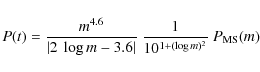
Method 3 was applied to a sample of 122 PN for which all necessary data was available (cf. Maciel et al. 2003). Again we selected disk planetary nebulae for which the best abundance data were available so as to keep the uncertainties to a minimum. The results are shown in Figs. 3 and 4 for Cases A and B, respectively. These results are similar to the age-metalllicity-radius method, in that most objects have ages lower than about 10 Gyr, and there is a sharp maximum in the probability distribution. However, its location depends on the estimated lifetimes as a function of the main sequence mass, being around 3-7 Gyr for Case A and 1-4 Gyr for Case B. From Case A to Case B the lifetimes of the more massive stars are decreased, so that the probability of finding stars at larger lifetimes decreases, and the whole peak moves to the left, as shown by Figs. 3 and 4.
![\begin{figure}
\par\includegraphics[angle=-90,width=9cm]{12499fg3.eps} \vspace*{4mm}
\end{figure}](/articles/aa/full_html/2010/04/aa12499-09/img33.png)
|
Figure 3: Age distribution of the central stars of planetary nebulae using a mass-N/O abundance relation (Case A). The estimated age uncertainty is shown in the upper right corner. |
| Open with DEXTER | |
![\begin{figure}
\par\includegraphics[angle=-90,width=9cm]{12499fg4.eps}
\vspace*{10mm}
\end{figure}](/articles/aa/full_html/2010/04/aa12499-09/img34.png)
|
Figure 4: The same as Fig. 3 for Case B. |
| Open with DEXTER | |
2.2b. Uncertainty analysis
An estimate of the uncertainties involved in Method 3 suggests that they are similar or
somewhat larger than in Methods 1 and 2. The basic relation is given by Eqs. (4) and (5), which
relate the central star masses and the N/O abundances. Although such a relation is
expected from theoretical models (see for example Renzini & Voli 1981; Marigo
2000, 2001; Perinotto et al. 2004), there is presently no
clearcut functional dependence between these quantities, which led Cazetta & Maciel
(2000) and Maciel (2000)
to propose a calibration based on the best parameters available. The
N/O ratio is determined relatively well, with uncertainties similar to
the O/H ratio or even better, namely, under 0.2 dex, as already
discussed. Adopting this value and also taking
the uncertainties in the coefficients of Eqs. (4) and (5) into
account, an upper limit of about 0.2 ![]() would be obtained for the mass uncertainty. However, a more realistic estimate
would be lower than this value, as suggested by the recent application of N/O masses to a
well-studied sample of CSPN by Maciel et al. (2008).
would be obtained for the mass uncertainty. However, a more realistic estimate
would be lower than this value, as suggested by the recent application of N/O masses to a
well-studied sample of CSPN by Maciel et al. (2008).
In that work, the derived masses were successfully compared with the
known mass distributions of CSPN and white dwarf stars, in order to
explain the relationship between the modified momentum of the CSPN
winds and the stellar luminosity. Some additional support to the N/O
masses comes from the re-analysis of Tinkler & Lamers (2002) of the central star masses determined by Kudritzki et al. (1997).
These results were based on a homogeneous set of parameters obtained
from Zanstra temperatures, dynamical ages, and evolutionary tracks. The
average masses obtained by Tinkler & Lamers (2002) for the same sample studied by Maciel et al. (2008)
and the N/O masses are in very good agreement. In view of these considerations, an average
uncertainty closer to
![]() would be more appropriate to Eqs. (4) and (5).
would be more appropriate to Eqs. (4) and (5).
Considering now the initial mass-final mass relation as given by Eq. (6), there are many
determinations of this relation in the literature (Vassiliadis & Wood 1993;
Marigo 2000, 2001; Marigo & Girardi 2007; Meng et al.
2008), which generally agree with each other within 0.1 to 0.2 ![]() ,
so that the
total uncertainties in the stellar masses are probably not affected much by this relation. As
a consequence, the average uncertainties in the indivdual CSPN ages correspond to a mass
uncertainty of at most 0.2
,
so that the
total uncertainties in the stellar masses are probably not affected much by this relation. As
a consequence, the average uncertainties in the indivdual CSPN ages correspond to a mass
uncertainty of at most 0.2 ![]() .
In fact, the main contribution to the age uncertainty
comes from to the age estimates as given by Eq. (7), and at this point the best procedure for
overcoming such a difficulty is to adopt some kind of parametrization, by considering Cases A
and B. Applying the mass uncertainty mentioned above, a formal age uncertainty would be about
3.1 and 4.7 Gyr for Cases A and B, respectively, considering a typical star of one solar mass at
the main sequence. These values can be considered as upper limits, as they were obtained using a
.
In fact, the main contribution to the age uncertainty
comes from to the age estimates as given by Eq. (7), and at this point the best procedure for
overcoming such a difficulty is to adopt some kind of parametrization, by considering Cases A
and B. Applying the mass uncertainty mentioned above, a formal age uncertainty would be about
3.1 and 4.7 Gyr for Cases A and B, respectively, considering a typical star of one solar mass at
the main sequence. These values can be considered as upper limits, as they were obtained using a
![]() mass uncertainty. Adopting the more reasonable value of about
mass uncertainty. Adopting the more reasonable value of about
![]() ,
the
average uncertainties would be 1.7 Gyr and 2.9 Gyr for Cases A and B, as shown by the error bars
in Figs. 3 and 4. Again, it should be stressed that we are interested in the age distribution,
rather than in individual ages, so that the general effect of the
uncertainties is expected to be less than indicated by the formal
uncertainties.
,
the
average uncertainties would be 1.7 Gyr and 2.9 Gyr for Cases A and B, as shown by the error bars
in Figs. 3 and 4. Again, it should be stressed that we are interested in the age distribution,
rather than in individual ages, so that the general effect of the
uncertainties is expected to be less than indicated by the formal
uncertainties.
2.2c. Binary CSPN
A final comment is appropriate on Method 3, concerning the possibility that a significant fraction of the PN may have originated from close binary stars. Current results are controversial, meaning that a very small number of binary PN are known, as discussed by De Marco (2009), while some investigations suggest that binaries constitute a much greater proportion of the galactic nebulae (see for example Miszalski et al. 2009; De Marco 2006, 2009; Moe & De Marco 2006). In view of these contradictory aspects, it is difficult to evaluate the effect of binarity on the present results. It would be expected that the age distribution would be displaced towards higher ages by only a small amount, as suggested by the good agreement of the results of our methods with the actual mass distribution of CSPN and white dwarf stars, as we will see in the next section.
3 The expected age distribution of the central stars of planetary nebulae
3.1 The white dwarf mass distribution
The expected age distribution of the CSPN can be estimated by analysing the much better known mass
distribution of the white dwarf stars. Since the average mass loss rates during the PN phase amount
to about
![]() to
to
![]() and the whole PN phase duration is about
and the whole PN phase duration is about
![]() to
to
![]() ,
the total mass lost during this phase is
,
the total mass lost during this phase is
![]() to
to
![]() ,
which is much less than the CSPN masses. Therefore, as a first
approximation, the mass distribution of the CSPN must be similar to
that of the white dwarfs, except for the very low-mass stars with
,
which is much less than the CSPN masses. Therefore, as a first
approximation, the mass distribution of the CSPN must be similar to
that of the white dwarfs, except for the very low-mass stars with
![]() .
Such stars are not expected from theoretical models, since main
sequence stars leading to white dwarfs with masses lower than about
.
Such stars are not expected from theoretical models, since main
sequence stars leading to white dwarfs with masses lower than about
![]() probably go directly to the white dwarf phase.
probably go directly to the white dwarf phase.
Recent work on the mass distribution of white dwarfs by Madej et al. (2004) and Kepler et al. (2007) have led to a distribution that is strongly peaked at about
![]() ,
as shown in Fig. 5 (cf. Madej et al. 2004).
This investigation was based on a large sample of about 1200 white
dwarfs, and it shows very few objects (about 5%) with masses higher
than about
,
as shown in Fig. 5 (cf. Madej et al. 2004).
This investigation was based on a large sample of about 1200 white
dwarfs, and it shows very few objects (about 5%) with masses higher
than about
![]() .
.
![\begin{figure}
\par\includegraphics[angle=-90,width=9cm]{12499fg5.eps}
\end{figure}](/articles/aa/full_html/2010/04/aa12499-09/img47.png)
|
Figure 5: Mass distribution of white dwarfs (Madej et al. 2004) and Gaussian fit. |
| Open with DEXTER | |
The white dwarf mass distribution can be well-fitted by a Gaussian probability density distribution
defined by

|
(8) |
where N(m) is the number of stars with mass m,
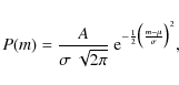
|
(9) |
where A = 0.90349,

|
(10) |
and
![\begin{figure}
\par\includegraphics[angle=-90,width=9cm]{12499fg6.eps}
\end{figure}](/articles/aa/full_html/2010/04/aa12499-09/img62.png)
|
Figure 6: Mass distribution of CSPN progenitor stars at the main sequence. |
| Open with DEXTER | |
Assuming that the star formation rate in the Galaxy has remained approximately constant along the
galactic lifetime, the age distribution of the CSPN can be estimated from the mass distribution of
their progenitor stars. To derive the age distribution of the observed CSPN, we adopt
Cases A and B considered previously. Considering that
![]() ,
we have for Case A
,
we have for Case A

|
(11) |
and for Case B
|
(12) |
where we have dropped the subscript MS from the mass. The obtained age distributions are shown in Fig. 7 for Cases A and B, respectively. Case A gives longer lifetimes for masses greater than one solar mass, which pushes the peak of the probability distribution to the right (2-3 Gyr), while for Case B these lifetimes are shorter, and the peak moves to the left (
![\begin{figure}
\par\includegraphics[angle=-90,width=9cm]{12499fg7.eps}
\end{figure}](/articles/aa/full_html/2010/04/aa12499-09/img66.png)
|
Figure 7: Age distribution of the progenitors of the central stars of planetary nebulae. Solid line: Case A, dashed line: Case B. |
| Open with DEXTER | |
For the sake of generality, we have also considered a quadratic
relation as in Eq. (6) with ![]() instead of a linear equation. In this case, we adopted
the constants a, b, and c from the recent work of Meng et al. (2008), taking the
metal abundance Z = 0.02. The central star mass is given by the minimum of
instead of a linear equation. In this case, we adopted
the constants a, b, and c from the recent work of Meng et al. (2008), taking the
metal abundance Z = 0.02. The central star mass is given by the minimum of
![]() and
and
![]() ,
where
a1 = 0.5716,
b1 = -0.04633,
c1 = 0.02878,
a2 = 1.1533,
b2 = -0.2422, and
c2 = 0.04091. In this case, the probability
,
where
a1 = 0.5716,
b1 = -0.04633,
c1 = 0.02878,
a2 = 1.1533,
b2 = -0.2422, and
c2 = 0.04091. In this case, the probability
![]() is given by
is given by
![]() .
As it turned out, the results of Fig. 7 are
not particularly sensitive to this assumption.
.
As it turned out, the results of Fig. 7 are
not particularly sensitive to this assumption.
3.2 The observed mass distribution of the central stars of planetary nebulae
The mass distributions of CSPN and white dwarfs have also been previously considered by Stasinska
et al. (1997) and Napiwotzki (2006). More recently, Gesicki & Zijlstra
(2007) analysed these distributions based on a dynamical method that allows mass
determinations within
![]() (cf. Gesicki et al. 2006).
The CSPN masses were
obtained for a sample of 101 objects from a relation between the
temperatures of the central stars and the dynamical age of the
surrounding nebulae. The ages were derived from a combination of recent
spectra, line ratios, and nebular sizes, using a photoionization model
to obtain the central star temperature. Theoretical tracks by Blöcker (1995) were used to derive the stellar masses. It turns out that both the CSPN and white dwarf distributions peak around
(cf. Gesicki et al. 2006).
The CSPN masses were
obtained for a sample of 101 objects from a relation between the
temperatures of the central stars and the dynamical age of the
surrounding nebulae. The ages were derived from a combination of recent
spectra, line ratios, and nebular sizes, using a photoionization model
to obtain the central star temperature. Theoretical tracks by Blöcker (1995) were used to derive the stellar masses. It turns out that both the CSPN and white dwarf distributions peak around
![]() as in Madej et al. (2004) and Stasinska et al. (1997),
although the white dwarf distribution shows a broader mass range. The
CSPN distribution shows essentially no objects with masses higher than
as in Madej et al. (2004) and Stasinska et al. (1997),
although the white dwarf distribution shows a broader mass range. The
CSPN distribution shows essentially no objects with masses higher than
![]() ,
while in the case of the DA white dwarfs, which are presumably the
offspring of H-rich CSPN, a few objects are observed with masses higher
than
,
while in the case of the DA white dwarfs, which are presumably the
offspring of H-rich CSPN, a few objects are observed with masses higher
than
![]() .
Although there may be some differences between the recently obtained
white dwarf mass distributions, as discussed by Gesicki & Zijlstra (2007), they all agree in that any sizable sample of CSPN is expected to have more objects with masses close to
.
Although there may be some differences between the recently obtained
white dwarf mass distributions, as discussed by Gesicki & Zijlstra (2007), they all agree in that any sizable sample of CSPN is expected to have more objects with masses close to
![]() .
These results are in good agreement with our own N/O masses, as discussed by Maciel et al. (2008).
.
These results are in good agreement with our own N/O masses, as discussed by Maciel et al. (2008).
Instead of adopting the white dwarf mass distribution, we may then use directly the mass
distribution of CSPN as recently derived by Gesicki and Zijlstra (2007). The mass
distribution is shown in Fig. 8, and can also be approximated as a Gaussian probability density distribution similar to Eq. (9), where we find
A = 0.89627,
![]() ,
and
,
and
![]() .
The corresponding probability distribution for CSPN is also shown in Fig. 8. Adopting again the same hypotheses as in Sect. 3.1, the CSPN age distributions are shown in Fig. 9
for Cases A and B, respectively. In this case, the peaks are located at
approximately 4-6 Gyr (Case A) and 2-4 Gyr (Case B).
.
The corresponding probability distribution for CSPN is also shown in Fig. 8. Adopting again the same hypotheses as in Sect. 3.1, the CSPN age distributions are shown in Fig. 9
for Cases A and B, respectively. In this case, the peaks are located at
approximately 4-6 Gyr (Case A) and 2-4 Gyr (Case B).
![\begin{figure}
\par\includegraphics[angle=-90,width=9cm]{12499fg8.eps}
\end{figure}](/articles/aa/full_html/2010/04/aa12499-09/img76.png)
|
Figure 8: Mass distribution of the central stars of planetary nebulae from Gesicki & Zijlstra (2007) and a Gaussian fit. |
| Open with DEXTER | |
![\begin{figure}
\par\includegraphics[angle=-90,width=9cm]{12499fg9.eps}
\end{figure}](/articles/aa/full_html/2010/04/aa12499-09/img77.png)
|
Figure 9: Age distribution of the CSPN progenitor stars from the observed mass distribution. Solid line: Case A, dashed line: Case B. |
| Open with DEXTER | |
4 Discussion
Some indication of the age distribution of CSPN may be obtained from the PN classification originally proposed by Peimbert (1976, 1990). According to this classification, the following approximate ages are attributed to the different PN types: type I (1 Gyr), type II (3 Gyr), type III (6 Gyr), and type IV (10 Gyr) (see for example Stasinska 2004, Table 7). Type IV are halo objects, which are rarer and presumably much older than the remaining types, which are located in the disk and bulge of the Galaxy. Since nebulae of types I-III constitute the vast majority of the known galactic PN, in this work we will not take the older, type IV nebulae into account.
Figure 7 shows the CSPN age distributions for Cases A and B using the mass distribution of white dwarfs (Madej et al. 2004), and Fig. 9 gives the corresponding distributions from the CSPN (Gesicki & Zijlstra 2007) mass distribution. The merged age distributions suggest a maximum around 2-6 Gyr for Case A and 1-4 Gyr for Case B. Again, the main conclusion that can be drawn is that a peaked distribution can be expected, but the location of the peak depends on the adopted assumptions. In principle, we would expect Case B to be more realistic than Case A (see the discussion of stellar lifetimes by Romano et al. 2005), so that the results of Sect. 3 would suggest a preferable range of 1-4 Gyr for the peak of the distribution. On the other hand, the results based on the empirical CSPN mass distribution are probably more accurate than those inferred from the white dwarf mass distribution, for the reasons mentioned in Sect. 3. Therefore, in view of these considerations, and taking the uncertainty analyses of Sects. 2.1c. and 2.2b. into account, we suggest that the peak of the age distribution is probably located around 2-4 Gyr, as shown in Fig. 9. We may then compare this distribution with the results of Sect. 2. Considering the uncertainties involved in the age determinations, which are estimated to be approximately in the range 1.0-2.0 Gyr, as discussed in Sect. 2, it can be concluded that all methods considered produce results reasonably in agreement with the expected age distribution. According to the discussion in Sect. 2, Methods 1 and 2 have similar results, as indicated by Figs. 1 and 2, but the age distribution of Method 2 is less strongly peaked than either of the distributions obtained in Sect. 3 (cf. Figs. 7 and 9). Since the uncertainties are similar, Method 1 is probably more accurate than Method 2.
At face value, the age distributions of Method 3 shown in Figs. 3 and 4 are very similar to the results of Fig. 9, especially if Case B is considered, as seems more appropriate. In other words, the best results are probably those by Method 3, Case B (Fig. 4), which show very good agreement with the results from the empirical mass distribution of CSPN, as shown in Fig. 9. Although the estimated uncertainty of Method 3 is larger, it is reassuring that the average distribution shows such remarkable agreement with the expected age distribution of CSPN. Therefore, our results obtained from completeley independent methods and sources of data are reasonably in agreement with each other, so that we can have an estimate of the age distribution of CSPN. Naturally, the details of the individual age determinations still need to be worked out.
AcknowledgementsWe are indebted to an anonymous referee, whose detailed comments helped improving the present paper. This work was partially supported by FAPESP and CNPq.
References
- Asplund, M. 2003, CNO in the universe, ed. C. Charbonnel, D. Schaerer, G. Meynet, ASP Conf. Ser., 304, 275 [Google Scholar]
- Asplund, M., Grevesse, N., Sauval, A. J., Allende-Prieto, C., & Kiselman, D. 2004, A&A, 417, 751 [NASA ADS] [CrossRef] [EDP Sciences] [Google Scholar]
- Asplund, M., Grevesse, N., & Sauval, A. J. 2006, Nucl. Phys. A, 777, 1 [NASA ADS] [CrossRef] [Google Scholar]
- Bahcall, J. N., & Piran, T. 1983, ApJ, 267, L77 [NASA ADS] [CrossRef] [Google Scholar]
- Bensby, T., Feltzing, S., & Lundström, I. 2004, A&A, 421, 969 [NASA ADS] [CrossRef] [EDP Sciences] [Google Scholar]
- Blöcker, T. 1995, A&A, 299, 755 [NASA ADS] [Google Scholar]
- Cahn, J. H., Kaler, J. B., & Stanghellini, L. 1992, A&AS, 94, 399 [NASA ADS] [Google Scholar]
- Cazetta, J. O., & Maciel, W. J. 2000, Rev. Mex. Astron. Astrophys., 36, 3 [Google Scholar]
- De Marco, O. 2006, IAU Symp., 234, ed. M. J. Barlow, & R. H. Méndez (CUP), 111 [Google Scholar]
- De Marco, O. 2009, PASP, 121, 316 [NASA ADS] [CrossRef] [Google Scholar]
- Edvardsson, B., Anderson, J., Gustafsson, B., et al. 1993, A&A, 275, 101 [NASA ADS] [Google Scholar]
- Feltzing, S., Holmberg, J., & Hurley, J. R. 2001, A&A, 377, 911 [NASA ADS] [CrossRef] [EDP Sciences] [Google Scholar]
- Gesicki, K., & Zijlstra, A. A. 2007, A&A, 467, L29 [NASA ADS] [CrossRef] [EDP Sciences] [Google Scholar]
- Gesicki, K., Zijlstra, A. A., Acker, A., et al. 2006, A&A, 451, 925 [NASA ADS] [CrossRef] [EDP Sciences] [Google Scholar]
- Gutenkunst, S., Bernard-Salas, J., Pottasch, S. R., Sloan, G. C., & Houck, J. R. 2008, ApJ, 680, 120 [Google Scholar]
- Hillebrand, L., Mamajek, E., Stauffer, J., et al. 2009, Cool stars, stellar systems and the Sun, 15th Cambridge Workshop, AIP Conf. Proc., 1094, 800 [Google Scholar]
- Idiart, T. P., Maciel, W. J., & Costa, R. D. D. 2007, A&A, 472, 101 [NASA ADS] [CrossRef] [EDP Sciences] [Google Scholar]
- Kepler, S. O., et al., 2007, MNRAS, 375, 1315 [NASA ADS] [CrossRef] [Google Scholar]
- Kudritzki, R.-P., Méndez, R. H., Puls, J., & McCarthy, J. K. 1997, IAU Symp., 180, ed. H. J. Habing, & H. J. G. L. M. Lamers (Kluwer), 64 [Google Scholar]
- Liu, X.-W. 2006, IAU Symp. 234, ed. M. J. Barlow, & R. H. Méndez (CUP), 219 [Google Scholar]
- Maciel, W. J. 2000, IAU Symp. 198, ed. L. da Silva, M. Spite, J. R. de Medeiros (ASP), 204 [Google Scholar]
- Maciel, W. J., & Costa, R. D. D. 2009, The Milky Way and the Local Group: Now and in the GAIA Era, Heidelberg Conference [Google Scholar]
- Maciel, W. J., Costa, R. D. D., & Uchida, M. M. M. 2003, A&A, 397, 667 [NASA ADS] [CrossRef] [EDP Sciences] [Google Scholar]
- Maciel, W. J., Lago, L. G., & Costa, R. D. D. 2005a, A&A, 433, 127 [NASA ADS] [CrossRef] [EDP Sciences] [Google Scholar]
- Maciel, W. J., Lago, L. G., & Costa, R. D. D. 2005b, in Planetary Nebulae as Astronomical Tools, ed. R. Szczerba, G. Stasinska, & S. K. Gorny, AIP Conf. Proc., 804, 246 [Google Scholar]
- Maciel, W. J., Lago, L. G., & Costa, R. D. D. 2006, A&A, 453, 587 [NASA ADS] [CrossRef] [EDP Sciences] [Google Scholar]
- Maciel, W. J., Keller, G. R., & Costa, R. D. D. 2008, Rev. Mex. Astron. Astrophys., 44, 221 [NASA ADS] [Google Scholar]
- Madej, J., Nalezyty, M., & Althaus, L. G. 2004, A&A, 419, L5 [NASA ADS] [CrossRef] [EDP Sciences] [Google Scholar]
- Marigo, P. 2000, in The evolution of the Milky Way, ed. F. Matteucci, F. Giovanelli (Kluwer), 481 [Google Scholar]
- Marigo, P. 2001, A&A, 370, 194 [NASA ADS] [CrossRef] [EDP Sciences] [Google Scholar]
- Marigo, P., & Girardi, L. 2007, A&A, 469, 239 [NASA ADS] [CrossRef] [EDP Sciences] [Google Scholar]
- Meng, X., Chen, X., & Han, Z. 2008, A&A, 487, 625 [NASA ADS] [CrossRef] [EDP Sciences] [Google Scholar]
- Miszalski, B., Acker, A., Moffat, A. F. J., Parker, Q. A., & Udalski, A. 2009, A&A, 496, 813 [NASA ADS] [CrossRef] [EDP Sciences] [Google Scholar]
- Moe, M., & De Marco, O. 2006, ApJ, 650, 916 [NASA ADS] [CrossRef] [Google Scholar]
- Napiwotzki, R. 2006, A&A, 451, L27 [NASA ADS] [CrossRef] [EDP Sciences] [Google Scholar]
- Nordström, B., Mayor, M., Andersen, J., et al. 2004, A&A, 418, 989 [NASA ADS] [CrossRef] [EDP Sciences] [Google Scholar]
- Peimbert, M. 1976, IAU Symp. 76, ed. Y. Terzian (Dordrecht: Reidel), 215 [Google Scholar]
- Peimbert, M. 1990, Rep. Prog. Phys., 53, 1559 [Google Scholar]
- Perinotto, M., Morbidelli, L., & Scatarzi, A. 2004, MNRAS, 349, 793 [NASA ADS] [CrossRef] [Google Scholar]
- Peña, M., Stasinska, G., & Gorny, S. K. 2005, in Planetary Nebulae as Astronomical Tools, ed. R. Szczerba, G. Stasinska, & S. K. Gorny, AIP Conf. Proc., 804, 243 [Google Scholar]
- Prantzos, N. 2008, IAU Symp. 254, ed. J. Andersen, J. Bland-Hawthorn, & B. Nordström (CUP), 381 [Google Scholar]
- Renzini, A., & Voli, M. 1981, A&A, 94, 193 [Google Scholar]
- Rocha-Pinto, H. J., Maciel, W. J., Scalo, J., & Flynn, C. 2000, A&A, 358, 850 [NASA ADS] [Google Scholar]
- Rocha-Pinto, H. J., Castilho, B. V., & Maciel, W. J. 2002, A&A, 384, 912 [NASA ADS] [CrossRef] [EDP Sciences] [Google Scholar]
- Rocha-Pinto, H. J., Rangel, R. H. O., Porto de Mello, G. F., Bragança, G. A., & Maciel, W. J. 2006, A&A, 453, L9 [NASA ADS] [CrossRef] [EDP Sciences] [Google Scholar]
- Romano, D., Chiappini, C., Matteucci, F., & Tosi, M. 2005, A&A, 430, 491 [NASA ADS] [CrossRef] [EDP Sciences] [Google Scholar]
- Soderblom, D. R. 2009, IAU Symp. 258, ed. E. Mamajek, D. R. Soderblom, & R. Wyse (Cambridge: Cambridge University Press), in press [Google Scholar]
- Stanghellini, L., Shaw, R. A., & Villaver, E. 2008, ApJ, 689, 194 [NASA ADS] [CrossRef] [EDP Sciences] [Google Scholar]
- Stasinska, G. 2004, in Cosmochemistry: The melting pot of the elements, ed. C. Esteban, R. J. García López, A. Herrero, & F. Sánchez (Cambridge: Cambridge University Press), 115 [Google Scholar]
- Stasinska, G. 2008, in Stellar Nucleosynthesis: 50 years after B2FH, ed. C. Charbonnel, & J.-P. Zahn, EAS Publ. Ser., 32, 173 [Google Scholar]
- Stasinska, G., Gorny, S. K., & Tylenda, R. 1997, A&A, 327, 736 [NASA ADS] [Google Scholar]
- Tinkler, C. M., & Lamers, H. J. G. L. M. 2002, A&A, 384, 987 [NASA ADS] [CrossRef] [EDP Sciences] [Google Scholar]
- Vassiliadis, E., & Wood, P. R. 1993, ApJ, 413, 641 [NASA ADS] [CrossRef] [Google Scholar]
- Zhang, C. Y. 1995, ApJS, 98, 659 [NASA ADS] [CrossRef] [Google Scholar]
All Figures
|
|
Figure 1: Age distribution of the central stars of planetary nebulae using an age-metallicity-galactocentric distance relation. The estimated age uncertainty is shown in the upper right corner. |
| Open with DEXTER | |
| In the text | |
|
|
Figure 2: Age distribution of the central stars of planetary nebulae using the age-metallicity relation of Rocha-Pinto et al. (2000). The estimated age uncertainty is shown in the upper right corner. |
| Open with DEXTER | |
| In the text | |
|
|
Figure 3: Age distribution of the central stars of planetary nebulae using a mass-N/O abundance relation (Case A). The estimated age uncertainty is shown in the upper right corner. |
| Open with DEXTER | |
| In the text | |
|
|
Figure 4: The same as Fig. 3 for Case B. |
| Open with DEXTER | |
| In the text | |
|
|
Figure 5: Mass distribution of white dwarfs (Madej et al. 2004) and Gaussian fit. |
| Open with DEXTER | |
| In the text | |
|
|
Figure 6: Mass distribution of CSPN progenitor stars at the main sequence. |
| Open with DEXTER | |
| In the text | |
|
|
Figure 7: Age distribution of the progenitors of the central stars of planetary nebulae. Solid line: Case A, dashed line: Case B. |
| Open with DEXTER | |
| In the text | |
|
|
Figure 8: Mass distribution of the central stars of planetary nebulae from Gesicki & Zijlstra (2007) and a Gaussian fit. |
| Open with DEXTER | |
| In the text | |
|
|
Figure 9: Age distribution of the CSPN progenitor stars from the observed mass distribution. Solid line: Case A, dashed line: Case B. |
| Open with DEXTER | |
| In the text | |
Copyright ESO 2010
Current usage metrics show cumulative count of Article Views (full-text article views including HTML views, PDF and ePub downloads, according to the available data) and Abstracts Views on Vision4Press platform.
Data correspond to usage on the plateform after 2015. The current usage metrics is available 48-96 hours after online publication and is updated daily on week days.
Initial download of the metrics may take a while.