| Issue |
A&A
Volume 512, March-April 2010
|
|
|---|---|---|
| Article Number | A69 | |
| Number of page(s) | 17 | |
| Section | Astronomical instrumentation | |
| DOI | https://doi.org/10.1051/0004-6361/200912107 | |
| Published online | 02 April 2010 | |
An analysis of outgassing pressure forces on the Rosetta orbiter using realistic 3D+t coma simulations
E. Mysen1 - A. V. Rodionov2 - J.-F. Crifo3
1 - Institute of Theoretical Astrophysics, University of Oslo,
PO Box 1029 Blindern, 0315 Oslo, Norway
2 -
Central Research Institute of Machine Building, Pionyerskaya St., 4,
Korolev, Moscow region 141070, Russia
3 -
CNRS, LATMOS, BP 3,
91371 Verrières-le-Buisson Cedex, France
Received 18 March 2009 / Accepted 7 December 2009
Abstract
A model for the interaction between a multicomponent Maxwellian
atmosphere and a
spacecraft is described. Multidimensional, time-dependent gasdynamical
simulations of the gas coma around
the recently reconstructed aspherical rotating nucleus of comet 67P/C-G
is used to analyze the outgassing pressure forces on the ESA spacecraft
Rosetta. The forces were in general found to be directed significantly
away from the cometocentric position vector of the spacecraft. It was
also found that in a maximum outgassing scenario at comet rendezvous,
the outgassing pressure force exceeds the gravitational attraction from
the nucleus in the cometocentric direction of the Sun. Furthermore, the
highly non-spherical pressure field was found to undergo very large
changes as the nucleus rotated. Still, it was possible to represent the
mean pressure field experienced by Rosetta by a fairly simple model,
which can be used for the determination of the comet mass and the
so-called oblateness coefficient c20
from the spacecraft Doppler signal. The oblateness coefficient
represents a type of asphericity of the gravity field. The
determination of the so-called triaxiality coefficient of the gravity
field c22 may require using the true pressure field instead of the mean pressure field.
Key words: celestial mechanics - hydrodynamics - space vehicles - comets: individual: 67P/Churyumov-Gerasimenko
1 Introduction
In 2014, the ESA probe Rosetta will reach the short-period comet 67P/Churyumov-Gerasimenko (hereafter called 67P). The spacecraft will approach the comet in the comet's own orbit, and the corresponding low relative velocity will make it possible to insert the probe into a bound orbit around its nucleus.
At the time of the approval of the mission, it
was believed that by placing the approach at a large heliocentric distance (
![]() AU)
one would deal with an inactive nucleus. Now it is widely believed
though that the formation of cometary comae (the nucleus ``activity'')
is due partly to solar-driven sublimation of water ice at
the nucleus surface, and partly to the diffusion of more volatile
molecules (for instance carbon monoxide) from subsurface regions.
Observations and physical simulations show that the former
process is limited to
AU)
one would deal with an inactive nucleus. Now it is widely believed
though that the formation of cometary comae (the nucleus ``activity'')
is due partly to solar-driven sublimation of water ice at
the nucleus surface, and partly to the diffusion of more volatile
molecules (for instance carbon monoxide) from subsurface regions.
Observations and physical simulations show that the former
process is limited to
![]() AU,
whereas the latter may extend far out into
the solar system (see the review of Prialnik et al. 2004).
Instrumental limitations generally preclude observations of the distant
activity (exceptions are e.g. comets Halley and Hale-Bopp, found active
up to 10 AU and 30 AU, respectively), hence it can often
happen that a nucleus which has substantial distant activity is
improperly designated as ``inactive''. Similar limitations also often
forbid the detection of molecules other than H2O even
at small rh in small comets. This is the case for 67P, of which only the
water activity has been observed - for
AU,
whereas the latter may extend far out into
the solar system (see the review of Prialnik et al. 2004).
Instrumental limitations generally preclude observations of the distant
activity (exceptions are e.g. comets Halley and Hale-Bopp, found active
up to 10 AU and 30 AU, respectively), hence it can often
happen that a nucleus which has substantial distant activity is
improperly designated as ``inactive''. Similar limitations also often
forbid the detection of molecules other than H2O even
at small rh in small comets. This is the case for 67P, of which only the
water activity has been observed - for
![]() AU. If all comets are
similar in origin, however, volatile molecule activity can also be expected at all distances
(see for instance Capria et al. 2004). Indeed, recent observations have revealed large dust grain
production at
AU. If all comets are
similar in origin, however, volatile molecule activity can also be expected at all distances
(see for instance Capria et al. 2004). Indeed, recent observations have revealed large dust grain
production at ![]() 3 AU from 67P (Marco Fulle and Jessica Agarwal, private communication, 2009) thus, in view
of the very large mass-to-area ratio of about 15 kg/m2 which is reached in a worst-case scenario,
it is possible that the Rosetta orbiter will
experience significant outgassing pressure forces at rendezvous.
3 AU from 67P (Marco Fulle and Jessica Agarwal, private communication, 2009) thus, in view
of the very large mass-to-area ratio of about 15 kg/m2 which is reached in a worst-case scenario,
it is possible that the Rosetta orbiter will
experience significant outgassing pressure forces at rendezvous.
A stated goal of the Rosetta Radio Science Investigations is the
determination of the nucleus' gravity field from Doppler data (Pätzold
et al. 2007). In other words, the gravity field of 67P can be
determined by the study of how the comet's gravity alters the
line-of-sight velocity of Rosetta in its orbit around the comet. The
cometocentric gravitational acceleration of an orbiting spacecraft can
be derived from the gravitational potential V, which for our purposes can be parameterized by the nucleus mass ![]() (treated in Mysen & Aksnes 2008) and the gravity coefficients c20 and c22,
to be defined later. In order to obtain these parameters, it is
essential to have a physical model that connects them to the observable
data. In the case of the Rosetta orbiter, this physical model must
include the outgassing pressure force from the rapidly expanding coma
or atmosphere around the comet's nucleus. Cometary dust poses a hazard
to the spacecraft, but does not contribute significantly to the
dynamics due to the low relative velocity between the dust particles
and the spacecraft (see Mysen & Aksnes 2006, and references
therein).
(treated in Mysen & Aksnes 2008) and the gravity coefficients c20 and c22,
to be defined later. In order to obtain these parameters, it is
essential to have a physical model that connects them to the observable
data. In the case of the Rosetta orbiter, this physical model must
include the outgassing pressure force from the rapidly expanding coma
or atmosphere around the comet's nucleus. Cometary dust poses a hazard
to the spacecraft, but does not contribute significantly to the
dynamics due to the low relative velocity between the dust particles
and the spacecraft (see Mysen & Aksnes 2006, and references
therein).
Below (1) we base our analysis on state-of-the-art computations of the near-nucleus coma for the first time and (2) we use parameters thoroughly compatible with the existing observations of 67P. On the other hand, to make the use of the computed pressure field easier (as far as possible) we investigate whether a simple deterministic model of acceptable precision (of the kind proposed by Scheeres et al. 2000) can exist for the pressure field.
1.1 Past celestial dynamics pressure force models
Several force models for the outgassing pressure effects on a cometary orbiter have been proposed previously. Models of this kind necessarily include (a) a gas outflow model to compute the gas parameters at any point from specific assumptions on the nucleus size, shape, rotation and gas production, and (b) algorithms to assess the force magnitude and direction from the local coma gas parameters. An analysis of the existing publications shows that in all cases these two components suffer from deficiencies. It is the purpose of the present paper to propose improved approaches for the 67P case.As a first example, in Scheeres et al. (2000) an expansion in orthogonal spherical harmonic
functions is fitted to the simulated outgassing pressure field
![]() of a
spherical nucleus,
probably derived from some kind of fluid dynamics computation
(unfortunately, the details are only referenced in unpublished work).
As with the force
of a
spherical nucleus,
probably derived from some kind of fluid dynamics computation
(unfortunately, the details are only referenced in unpublished work).
As with the force ![]() ,
it is taken equal (after misprint correction) to
,
it is taken equal (after misprint correction) to
![]() ,
where AS/C is the probe cross-section and
,
where AS/C is the probe cross-section and ![]() the cometocentric unit radial vector. That is, the pressure force is
assumed to act mainly away from the nucleus, and the force's temporal
variations as the nucleus rotates are not accounted for.
the cometocentric unit radial vector. That is, the pressure force is
assumed to act mainly away from the nucleus, and the force's temporal
variations as the nucleus rotates are not accounted for.
In the second example (Byram et al. 2007) the gas coma is modelled as a series of twenty discrete
narrow conical jets attached to a rotating
ellipsoidal nucleus, all having the same radial flow velocity V,
but differing openings and gas mass fluxes
![]() (kg/s)
assumed to vary with the (time-dependent) solar zenith angle at their base
(kg/s)
assumed to vary with the (time-dependent) solar zenith angle at their base ![]() .
In support of this assumption it is stated that such a coma structure has been ``identified'' in the 2004 flyby images
of the comet P/Wild 2. Let us observe here that these are images of the dust (not gas) coma,
and that no supporting dusty gasdynamical computation is mentioned in support of this
``identification''. The aerodynamic force is taken to be
.
In support of this assumption it is stated that such a coma structure has been ``identified'' in the 2004 flyby images
of the comet P/Wild 2. Let us observe here that these are images of the dust (not gas) coma,
and that no supporting dusty gasdynamical computation is mentioned in support of this
``identification''. The aerodynamic force is taken to be

|
(1) |
where ri and riN are the distance to the apex of the jet i of the spacecraft and of the nucleus surface respectively, ei(t) is the (time-dependent) unit vector from this apex to the probe, and
1.2 Lessons from past gasdynamical model results
More than a decade of 2D, 3D and 3D+t gasdynamical simulations of comae by various authors using various computational techniques (see the review of Crifo 2004a) have clearly revealed how gas outflowing in a vacuum from a geometrically irregular, rotating solid builds up a huge atmosphere around it. There are four essential characteristics.
In the first place, the surface topography of the object plays a strong role (as common sense evidences) upon the outflow, attaching specific flow structures to many topographic details (such as concavities). This is due in part to shadowing effects and in part to flow obstacle effects. The effect is that the rotation of the central object renders the gas coma flow pattern fully time-dependent (quasi-periodic). Furthermore, since gravitational asphericities are in general associated with such topographic details, the effect may introduce a correlation between pressure force variations and gravity variations. Let us stress that this topography control occurs if the gas is emitted from the whole object or from several discrete areas. Thus, Crifo et al. (2002) showed that comet Halley's dust coma fine structures are equally well reproduced whether one postulates a uniform or a non-uniform gas production. In Crifo (2004) the Wild 2 synthetic dust coma image is compared to a dusty gasdynamical computation of the near-nucleus coma around a random shaped nucleus, suggesting immediately that the Wild 2 claimed (without any supporting modelling) ``active areas'' are nothing but the signatures of Wild 2 non-smooth surface. This will be checked in the future. By smoothing their model nuclei, both Sheeres et al. (2000) and Byram et al. (2007) eliminate this essential topography control.
Secondly, it is a fundamental property of inhomogeneous vacuum outflows that they are structured by a pattern of shocks - the effect is well documented e.g. in multiple-thrusters rocket motors. This effect (also called jet-jet interaction) renders the relation between source pattern and outflow structure non-intuitive. Thus, if the discrete gas sources of Byram et al. (2007) really existed, the jet-jet interactions would create a very disordered gas coma instead of their physically impossible independent rigid gas cones. In particular, even if all jets had initially the same velocity, a considerable velocity dispersion would appear (subsonic and supersonic areas). Furthermore, as the jet fluxes vary with nucleus orientation, the resulting ``very disordered'' structure and the velocity dispersion will change dramatically. Thus, while the Byram et al. (2007) coma changes during the rotation (as requested), the changes are over-simplified compared to those of a real coma. At this point it is instructive to note that these authors cite a paper by Crifo et al. (1994) in support of their approach, which precisely evidences the jet-jet interaction, whereby the impossibility of their model is demonstrated.
Third, because the illumination of the surface varies during its rotation, so does its temperature field, hence, even if there existed a permanent corotating surface gas flux pattern linked to the topography, still the initial gas temperature and velocity would change considerably with the solar zenith angle: a constant velocity in all jets during the rotation is a physical impossibility.
Finally, in view of the enormous difference in inertia between molecules and grains, coma dust patterns are non-trivial tracers of the surface gas emission. Hence, claims to visually infer gas sources from dust coma images without any supporting dusty gasdynamic computations must be firmly discarded. This is true for comet Wild 2 beyond any possible doubt, as stated above. To be sure, an inhomogeneity of surface gas production is possible in principle, but this can only be confirmed by coupled dust/gas dynamical simulations that reproduce the images.
Below we do not assume a strong inhomogeneity of the nucleus for two reasons. First, as discussed above, most advocations in the literature of strongly localized gas emission due to a strong nucleus inhomogeneity are merely opinions, not conclusions from physical model fits of the observations. Let us observe here that the flyby images of comet Tempel 1 evidence different areas of production for different molecules (Feaga et al. 2007); still the total coma density does not exhibit dramatic changes with position on the day side. Secondly, a significant inhomogeneity of gas production does appear even when assuming a homogeneous nucleus, due to the effect of solar illumination. Thus our computed coma is representative of any possible gas coma. However, it is true that an extreme instance where the total gas production would be localized in a few separated areas might lead to locally stronger pressures than computed here.
1.3 The problem of the force model
It is well known that a solid placed in a gas flow undergoes a force with components parallel (drag) and transverse (lift) to the flow. As described above, earlier works took the latter to be negligible on an intuitive basis, but a quantitative proof of the validity of this assumption is still missing. Another problem, probably specific to the large size of the Rosetta orbiter, is that this size is not necessarily smaller than the gas mean free path. For 67P at perihelion, simple estimates show that this is certainly not the case close to the nucleus. As the gas-spacecraft relative velocity is supersonic, it follows that in such a case, the gas parameters at the spacecraft differ from those of the unperturbed flow (an attached or a detached shock wave may appear). Below we mostly address the lift vs. drag problem for which we rederive the pressure field equations from first principles. As with the question of whether or not the gas mean free path is much larger than the size of the spacecraft, we here only delineate that region of the coma (at 3 AU) where this is expected to be the case.
2 Interaction between coma and spacecraft
Let us consider a pure gas (i.e. containing identical molecules), and let us in addition
assume that the gas density is large enough for the molecule velocity distribution to
be well represented by a drifting Maxwellian, but small enough
that the mean free path of the molecules is significantly larger than the spacecraft, an assumption which will
be motivated and tested later. Adopting a cometocentric gas outflow
velocity V on the order of 0.65
![]() (see Fig. 9)
and a mass of the target comet of
(see Fig. 9)
and a mass of the target comet of
![]() (Davidsson & Gutierrez 2005), the
cometocentric velocity of the Rosetta orbiter at a close cometocentric distance
(Davidsson & Gutierrez 2005), the
cometocentric velocity of the Rosetta orbiter at a close cometocentric distance
![]() (
(
![]() being the mean radius of the nucleus according to Lamy et al. 2007)
is
being the mean radius of the nucleus according to Lamy et al. 2007)
is
![]() .
Therefore the distribution
of relative velocity
.
Therefore the distribution
of relative velocity ![]() between the orbiter and the gas is determined by
between the orbiter and the gas is determined by ![]() ,
and the Maxwellian velocity distribution (Valorge 1995)
,
and the Maxwellian velocity distribution (Valorge 1995)

|
(2) |
by setting

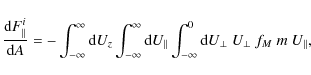
where the subscripts
To compute the pressure force on a spacecraft, it is convenient to represent it by a polyhedron and to sum the pressure forces exerted on each face of the polyhedron. Here we will further assume that this polyhedron is convex. That is to say, the whole half-space in front of each face is unobstructed by other faces of the spacecraft (thus also no face can receive molecules scattered from other faces). Then the pressure force due to any face is equal to the force exerted on one side of an isolated flat plate, computed with an appropriate area and orientation. Below, we will distinguish for convenience between ``front side plates'' and ``rear side plates''. That is, for a plate where both sides are exposed to gas pressure (as is the case in a Maxwellian gas), one is free to decide which side is ``front''. The other side then automatically becomes the ``rear'' side. It is important to note that once defined, this definition of ``front'' and ``rear'' remains fixed, independent of how the spacecraft is oriented with respect to the flow of the coma.

|
Figure 1:
A flat plate is seen from its side.
The plate moves with a velocity |
| Open with DEXTER | |
2.1 Pressure force on a front side flat plate
Let us consider the elementary area ![]() of the front side of a flat plate
moving with a velocity
of the front side of a flat plate
moving with a velocity ![]() relative to the atmosphere, with
relative to the atmosphere, with
![]() as the unit vector normal
to
as the unit vector normal
to ![]() .
Let
.
Let
![]() be a unit vector parallel to the plate, lying in the plane spanned
by
be a unit vector parallel to the plate, lying in the plane spanned
by ![]() and
and ![]() .
The force
.
The force
![]() experienced by
experienced by ![]() is due to the pressure
of the impacting molecules and to the recoil from the re-emitted particles. We do not consider here the case where
part of or all the impinging molecules would be condensed on the surface (for such a case, see e.g. Crifo 1995).
We will also assume that the plate is perfectly smooth, in the sense that the flux of the reemitted molecules
is symmetrical with respect to the incidence plane (
is due to the pressure
of the impacting molecules and to the recoil from the re-emitted particles. We do not consider here the case where
part of or all the impinging molecules would be condensed on the surface (for such a case, see e.g. Crifo 1995).
We will also assume that the plate is perfectly smooth, in the sense that the flux of the reemitted molecules
is symmetrical with respect to the incidence plane (
![]() ).
Then,
).
Then,
![]() has the form
has the form

where Tw is the plate temperature, and
|
(5) |
where the superscripts (i) and (r) denote the contributions from the incident molecules and from the re-emitted molecules respectively.
If we calculate the pressure exerted by the incoming gas molecules
following the Maxwellian velocity distribution, we obtain for the force
per unit area along ![]()

yielding
| |
= | 
|
|
| (7) |
Here

|
(8) |
and the pressure force from the incoming gas molecules is dependent on the flow Mach number M through the speed ratio s

where
resulting in
| |
= | 
|
|
| (11) |
There is some uncertainty (Harrison & Swinerd 1996) related to what happens to the gas molecules after they strike a spacecraft surface, but in any case, mass is conserved. Therefore, assuming that there is no condensation of molecules at the surface, the expression for the number of gas molecules striking the surface per unit time will be useful:
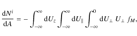
which gives
| |
= | ||
| (13) |
The contribution from the molecules leaving the surface,

|
(14) |
in which

|
(15) |
where

|
(16) |
is the thermal momentum of a gas molecule leaving the plate with temperature Tw. The definition
|
(17) |
completes the parametrization where the contribution from both the incoming molecules as well as from those leaving the surface have been accounted for. Note that
Since the two directions of greatest interest here for the pressure force really are
![]() and
and
![]() ,
we will use the force per unit area representation
,
we will use the force per unit area representation
derivable from Eq. (4) with the use of the relation

As the pressure force coefficients will obey
the attack angle need only be defined in the range

![$\displaystyle +\sqrt{\pi}~s\cos\vartheta{}~\left[~1+{\rm erf}(s\cos\vartheta)\right] \bigg\}.$](/articles/aa/full_html/2010/04/aa12107-09/img114.png)
For the force component normal to the flat plate we get
where
with
and

These expressions correspond to those of Schaaf & Chambré (1958) as given in Moore & Sowter (1991) if projected along the
At this point we may note that the mass dependence of the force due to the inflowing molecules is
contained in ![]() and s, which means that if the incoming gas is a mixture of molecules,
it will be in general sensitive to changes
of the molecular composition with position in the coma.
and s, which means that if the incoming gas is a mixture of molecules,
it will be in general sensitive to changes
of the molecular composition with position in the coma.
A significant simplification occurs in the so-called hypersonic limit
![]() .
In this case,
.
In this case,
![]() ,
whereby it can be shown that Eqs. (21)
and (23) are reduced to
,
whereby it can be shown that Eqs. (21)
and (23) are reduced to

and

where
|
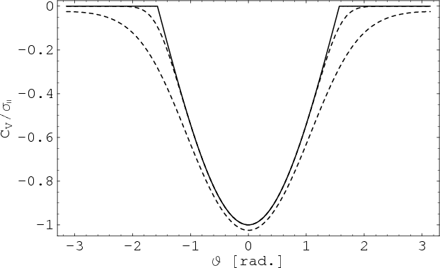
Figure 2:
The pressure force coefficient CV of Eq. (21) is given for different values of s, dashed lines. From bottom to top we have s=1, s=3, and
|
| Open with DEXTER | |

|
Figure 3:
From bottom to top, |
| Open with DEXTER | |
If the hypersonic approximation is met, four important implications appear. First, the
front side part of
the total force, Ff, is a function of the total mass density, whereby Eq. (18) can be used with ![]() as the total mass density; thus, Ff is insensitive to the molecular composition.
If this is not the case, the contributions of each kind of the molecules must be summed, using
its fractional mass density and speed ratio (not anymore related to M - the mixture Mach number -
by the Eq. (9)). Secondly, Ff
is also independent from the coma temperature, which therefore does not
need to be accurately assessed: it is only
necessary to make sure that it is low enough. Third, it is also
independent from the
spacecraft surface temperature (which is anyway probably monitored
in-flight). Fourth and most importantly, it is easy to see that Ff is in this
case the same as the one obtained if the molecules were all at rest with respect to one another.
Thus, the velocity dispersion playing no role, any velocity distribution - not necessarily a
Maxwellian - yields the same
result: the gas need not be in fluid regime. We return to this fundamental result below.
as the total mass density; thus, Ff is insensitive to the molecular composition.
If this is not the case, the contributions of each kind of the molecules must be summed, using
its fractional mass density and speed ratio (not anymore related to M - the mixture Mach number -
by the Eq. (9)). Secondly, Ff
is also independent from the coma temperature, which therefore does not
need to be accurately assessed: it is only
necessary to make sure that it is low enough. Third, it is also
independent from the
spacecraft surface temperature (which is anyway probably monitored
in-flight). Fourth and most importantly, it is easy to see that Ff is in this
case the same as the one obtained if the molecules were all at rest with respect to one another.
Thus, the velocity dispersion playing no role, any velocity distribution - not necessarily a
Maxwellian - yields the same
result: the gas need not be in fluid regime. We return to this fundamental result below.
2.2 Pressure force on a rear side flat plate
A rear side plate has its surface normal vector in the opposite direction to that of a ``front side'' plate parallel to it, independently from the orientation of the spacecraft with respect to the coma flow.
As our previously derived formulas for
![]() are applicable
for all attack angles
are applicable
for all attack angles ![]() ,
the force
,
the force
![]() due to the rear side is equal in magnitude
and opposite in direction to that computed above for an attack angle
due to the rear side is equal in magnitude
and opposite in direction to that computed above for an attack angle
![]() :
:

where
It is clear that in the hypersonic limit the simplifications found for the front side of the plate,
![]() ,
also apply to
,
also apply to
![]() .
.
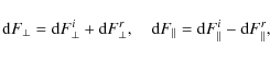
2.3 Total force from both sides of a flat plate
The ``front side'' and ``rear side'' elements of a spacecraft do not
necessarily have to be equivalent in temperature, nor does there have
to be a corresponding rear plate parallel or of the same size to every
front plate. For the present application however, our spacecraft shape
model is constructed so it can be subdivided into pairs of front side
and back side plates parallel to one another and with the same area. In
this case, it is convenient to treat it as
a collection of isolated plates (with both sides exposed to the gas).
The total force acting on an isolated flat plate,
![]() ,
is the sum of
,
is the sum of
![]() and
and
![]() given by Eqs. (4) and (28) respectively:
given by Eqs. (4) and (28) respectively:
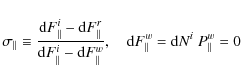
Defining the pressure field coefficients
![\begin{displaymath}
\frac{\sum{}{\rm d}\vec{F}}{{\rm d}A}=\varrho{}~V^2~\left[~\...
...right)~\vec{u}_{V}+\left(\sum{}C_{N}\right)~\vec{n}_f~\right],
\end{displaymath}](/articles/aa/full_html/2010/04/aa12107-09/img147.png)
it can easily be reasoned from Eqs. (19) and (29) that
and
For s > 3 we have the ``weak'' hypersonic expressions
which is

|
(34) |
|
(35) |
and

where the last term in Eq. (36) has been retained because of the uncertainty in the value of the ratio Tf/T.
For the present application to Rosetta, we will assume that the thermal design of the
spacecraft ensures approximate surface isothermicity, whereby
![]() ,
hence
,
hence

an expression that in accordance with the physical situation changes sign if
has been retained (``weak hypersonicity'') as Tf/T ratio's value is uncertain.
Based on Eqs. (30), (33) and (37)
we propose as a first attempt to interpret the radiometric data from
Rosetta that three estimation parameters for the description of the
interaction between spacecraft and coma can be

|
(39) |
Hopefully, applications will show that they are fairly constant. Otherwise the parameters above can be allowed to change over time to a certain extent. In Moore & Sowter (1991), where the last term of Eq. (37)

|
(40) |
Interestingly, this dependency of the normal accommodation coefficient will reintroduce a
As with Ff and Fb
the total force is independent of the coma temperature in the
hypersonic limit, and hence from the flow regime of the gas. However,
for Rosetta it may be that this condition is only partly met as
discussed precedingly, leaving in Eq. (37) the term dependent on
![]() ,
i.e.,
on the mass of the gas molecule. In this case we need to know
,
i.e.,
on the mass of the gas molecule. In this case we need to know
![]() for each different chemical species to calculate this component of the force.
In navigation and radio science, where scientific quantities are found by inverting
radiometric data from the spacecraft (Pätzold et al. 2007), only the properties of the chemical species which
contributes the most can be found. That is, if we can find a proper parametrization of
for each different chemical species to calculate this component of the force.
In navigation and radio science, where scientific quantities are found by inverting
radiometric data from the spacecraft (Pätzold et al. 2007), only the properties of the chemical species which
contributes the most can be found. That is, if we can find a proper parametrization of
![]() ,
we do not
necessarily have to operate with one such set of parameters for each chemical species. Of course, this simplification
does not hold if the probe enters a region during the tracking interval where the dominant contributor to the
pressure shifts from one species to another.
,
we do not
necessarily have to operate with one such set of parameters for each chemical species. Of course, this simplification
does not hold if the probe enters a region during the tracking interval where the dominant contributor to the
pressure shifts from one species to another.
In this paper, where the molecules CO and
![]() are considered and the
CO pressure usually dominates, we will make the approximation
are considered and the
CO pressure usually dominates, we will make the approximation

|
(41) |
As a result, we only need a proper description of the sum
Although our coefficients in Eq. (30)
are to a great extent determined by the defined parametrization, we
will nevertheless conclude that there is little a priori evidence for
the hypothesis of a pressure force on a cometary orbiter that acts
mainly in the direction away from the comet nucleus in general, as
assumed in Weeks (1995), Scheeres et al. (2000) and Byram
et al. (2007). That is, ![]() is zero for all attack angles
is zero for all attack angles
![]() only if there is full accommodation in all directions and the
spacecraft temperature is zero (unless, of course, the possibilities
only if there is full accommodation in all directions and the
spacecraft temperature is zero (unless, of course, the possibilities
![]() also are considered). This represents the most important property of
the presented simple model: it does not exclude forms of interaction
between the gas molecules and the spacecraft.
also are considered). This represents the most important property of
the presented simple model: it does not exclude forms of interaction
between the gas molecules and the spacecraft.
2.4 Rosetta's effective pressure force area
Let us define
![]() as the angle between the relative velocity vector
as the angle between the relative velocity vector ![]() and the unit vectors normal to the solar cell arrays with a total area
and the unit vectors normal to the solar cell arrays with a total area
![]() .
Also, let one surface of the bus with an area of
.
Also, let one surface of the bus with an area of
![]() point in the same direction as the solar cell arrays. Finally, assume that the bus area in the
point in the same direction as the solar cell arrays. Finally, assume that the bus area in the ![]() direction is
direction is
![]() when
when
![]() ,
i.e., when the solar cell arrays are not exposed to the pressure field. With the use of Eqs. (33) and (37)
we are now in a position to plot the effective outgassing pressure
force area of Rosetta in different directions. The directions used will
be the drag direction
,
i.e., when the solar cell arrays are not exposed to the pressure field. With the use of Eqs. (33) and (37)
we are now in a position to plot the effective outgassing pressure
force area of Rosetta in different directions. The directions used will
be the drag direction
![]() and the orthogonal lift direction
and the orthogonal lift direction ![]() (Fig. 1), related to a vector
(Fig. 1), related to a vector ![]() normal to a spacecraft surface through
normal to a spacecraft surface through
| (42) |
The contribution to the drag force from both the back side and front side of a spacecraft area
![\begin{displaymath}
\frac{\sum{}{\rm d}\vec{F}_D}{{\rm d}A_f} = \varrho{}V^2 \ve...
...(\vartheta_f)+~\cos\vartheta_f~\sum{}C_N(\vartheta_f)~\right].
\end{displaymath}](/articles/aa/full_html/2010/04/aa12107-09/img185.png)
Likewise, for the lift component
![\begin{displaymath}
\frac{\sum{}{\rm d}\vec{F}_L}{{\rm d}A_f} = \varrho{}V^2 \vec{u}_L~\left[~\sin\vartheta_f~\sum{}C_N(\vartheta_f)~\right].
\end{displaymath}](/articles/aa/full_html/2010/04/aa12107-09/img186.png)
Included as Fig. 4 is the effective area of Rosetta in the drag direction, based on Eq. (43). A typical value of

|
Figure 4:
The figure illustrates effective areas of Rosetta in the drag
direction: total (solid), without bus (dotted), or with the spacecraft
temperature set to
|
| Open with DEXTER | |

|
Figure 5:
The lift to drag ratio is shown above as a function of the attack angle |
| Open with DEXTER | |
3 Comet 67P model
The only reliable way to predict the behaviors of the important functions
![]() and V
of the previous section is to base the predictions on state-of-the art
computations of the 3D+t gas coma, making sure that all adopted
parameters are fully compatible with the present information
available on the 67P nucleus, summarized in
Lamy et al. (2007). To be sure, considerable uncertainty persists on the properties of this nucleus.
In particular, the CO production rate cannot be measured because
its upper-limit lies below the detection limit of existing ground-based instruments, and the nucleus shape
and perhaps rotation parameter are provisory.
One can see the evolution in the best-fit nucleus parameters by comparing
the present shape and coma properties (Figs. 7-9) with those given in
Crifo et al. (2004b), which were based on 2002 data (let
us remind that 67P has a period of about 6.5 years, hence new data are acquired every six to seven years).
While there is an unavoidable uncertainty in the present parameters we can warrant that our assumptions are compatible
with all existing
observations by basing our parameter choice on Lamy et al. (2007),
as opposed to assumptions which are in direct conflict with the
observations, as those of a spherical or ellipsoidal nucleus shape. By
using a 3D + t gasdynamical approach, we can guarantee
the robustness of the physical model, as opposed to using algorithms
which rely on untenable concepts, as a corotating rigid gas coma
pattern.
and V
of the previous section is to base the predictions on state-of-the art
computations of the 3D+t gas coma, making sure that all adopted
parameters are fully compatible with the present information
available on the 67P nucleus, summarized in
Lamy et al. (2007). To be sure, considerable uncertainty persists on the properties of this nucleus.
In particular, the CO production rate cannot be measured because
its upper-limit lies below the detection limit of existing ground-based instruments, and the nucleus shape
and perhaps rotation parameter are provisory.
One can see the evolution in the best-fit nucleus parameters by comparing
the present shape and coma properties (Figs. 7-9) with those given in
Crifo et al. (2004b), which were based on 2002 data (let
us remind that 67P has a period of about 6.5 years, hence new data are acquired every six to seven years).
While there is an unavoidable uncertainty in the present parameters we can warrant that our assumptions are compatible
with all existing
observations by basing our parameter choice on Lamy et al. (2007),
as opposed to assumptions which are in direct conflict with the
observations, as those of a spherical or ellipsoidal nucleus shape. By
using a 3D + t gasdynamical approach, we can guarantee
the robustness of the physical model, as opposed to using algorithms
which rely on untenable concepts, as a corotating rigid gas coma
pattern.
The main model parameters are summarized in Table 1. We call them ``maximum model'' because they correspond to the upper limits of the total water and CO production rates. Evidently, the real conditions could as well be those of minimum production rates, which are an order of magnitude smaller - our scenario is in this sense a worst-case scenario from the point of view of pressure effect on the orbiter. However, as discussed below, the surface distribution of these fluxes also influences the pressure and at this point in time it is not known whether our present assumptions are worst-case assumptions or not.
Table 1: Comet 67P model parameters.
3.1 Nucleus model
Using HST images of the comet, Lamy et al. (2007)
have been able to extract an approximate size, shape, and rotation mode of this nucleus. Figure 6
shows that, as all imaged cometary nuclei, the nucleus of 67P appears to be small (km size) and very irregular in shape.
We have adopted the shape of Lamy et al. (2007), and - consistently - their rotation model.
The nucleus radii are distributed around
![]() km.
The rotation is uniaxial and periodic with a period P=12.55 h.
The constant angle between the cometocentric direction
of the Sun and the axis of rotation is
km.
The rotation is uniaxial and periodic with a period P=12.55 h.
The constant angle between the cometocentric direction
of the Sun and the axis of rotation is
![]() .
Uniaxial rotation
has been inferred from the presently existing lightcurves by Lamy et al. (2007), but
a more realistic mode should not be entirely excluded.
.
Uniaxial rotation
has been inferred from the presently existing lightcurves by Lamy et al. (2007), but
a more realistic mode should not be entirely excluded.
| Figure 6: Present best-fit shape of the comet 67P nucleus. The largest diameter is about 5 km. The uncertainty is probably on the order of the magnitude of the topographic features. The corresponding best-fit monoaxial rotation is about the z-axis. The model will be periodically improved as new observational data are accumulated. After Lamy et al. (2007). |
|
| Open with DEXTER | |
The surface flux Z(CO) at any point with the solar
zenith angle ![]() is given by:
is given by:
![\begin{displaymath}Z({\rm CO}) = Q_{{\rm CO}}\left(\frac{A_0}{{\cal A}_{\rm ext}...
...(1 -A_0) ~{\rm max}[\cos{z_\odot},0.]}{{\cal A}_\odot}\right), \end{displaymath}](/articles/aa/full_html/2010/04/aa12107-09/img208.png)
|
(45) |
where
As stated precedingly, other assumptions with respect to the surface distribution of the ice and of the CO emission could have been made, because at the present time there is no observational constraint on it. For instance, both could have been assumed localized in small areas of the nucleus, leading to a much more contrasted gas coma structure. It would certainly be interesting to investigate in the future the implications for the pressure force field.
3.2 Molecular outflow model
The vacuum outflow of the molecules emitted by the nucleus is computed using the gasdynamical approach described in Rodionov et al. (2002), except that the method of solutions here is more powerful than the one described there, as one true time-dependent solutions is acquired (in lieu of a succession of steady state solutions). Thus, the time dependent tridimensional Euler Equations governing the gas outflow are solved by the shock-capturing Godunov method, using periodic boundary conditions for the integration over time. The time mesh is 1/72 of a rotation period, hence the solution consists of a set of 72 3D files. A brief description of this new family of solutions is given in Rodionov and Crifo (2006). The adequacy of Eulerian Equations for the present parameter choice and the presently considered cometocentric distances will be discussed below.4 Properties of the computed 3D+t gas coma
The time-dependent, periodic but non-co-rotating structure of the coma can be seen on Fig. 7, which shows snapshots of the total gas density in the rotation equatorial plane at nine equispaced times during one rotation period. One notes a clear day-to-night asymmetry, due in part to our assumed (modest) solar dependence of the CO flux, and in part to the solar-driven water production. Also evident on the figure is the correlation between density structures and nucleus topography, and the resulting time-dependence of the gas density at any point.![\begin{figure}
\par\includegraphics[scale=0.25,angle=-90]{12107f71.eps}\hspace*{...
...\hspace*{4mm}
\includegraphics[scale=0.25,angle=-90]{12107f79.eps}
\end{figure}](/articles/aa/full_html/2010/04/aa12107-09/img216.png)
|
Figure 7: Variation of the total mass density in the equatorial plane during the rotation. From left to right and from top to bottom: isocontours of Log10 (mass density, kg/m3) in the equatorial plane are shown every 1/9 of the rotation period (i.e., every 1.4 h.) The projected Sun direction is to the right. Notice the clockwise rotation of the nucleus cross section. On this and the two next figures, references and dates appear at the bottom left of each panel for safety of identification: the reader must overlook them. The dust contribution has not been included. |
| Open with DEXTER | |
To have a better feeling about the 3D structure of the coma and about its compositional variability, Fig. 8 shows the H2O and CO density distributions in the equatorial plane and in one meridional plane at rotation phase 0. It is clear that there is a very strong day-to-night change in the chemical composition due to the different physical origin of the molecules. Notice that the two patterns depend on one another, since under the conditions of interest here, the two species are closely coupled together by collisions and form a single fluid. As a consequence, if only water or only CO was produced, their coma patterns would differ from the present ones, because the distribution of surface gas flux would be different.
![\begin{figure}
\par\includegraphics[width=17cm,clip]{12107f08.eps}
\end{figure}](/articles/aa/full_html/2010/04/aa12107-09/img217.png)
|
Figure 8: Log10 of the H2O ( upper panels) and CO ( lower panels) density in two orthogonal planes at rotation phase 0. The projected Sun direction is to the right on the X-axis ( right panels) or at 200 to the X-axis ( left panels). The total density shown on Fig. 7 ( upper left panel) is the sum of the two present right panel densities. |
| Open with DEXTER | |
Figure 9 shows the distribution of the flow velocity and the flow Mach number in the same planes. There is not much day-to-night asymmetry in the Mach number, a general property of inviscid flows, but there is a very large difference in the flow velocity, due to the strong day-to-night surface temperature asymmetry. This temperature asymmetry is controlled in our model by the parameter Fs. Our present value for this parameter is probably a minimum, yielding a probable maximum day-to-night temperature asymmetry.
![\begin{figure}
\par\includegraphics[width=16.5cm,clip]{12107f09.eps}
\vspace*{-2mm}
\end{figure}](/articles/aa/full_html/2010/04/aa12107-09/img218.png)
|
Figure 9: Velocity ( upper panels) and Mach number ( lower panels) in two orthogonal planes at rotation phase 0. The projected Sun direction is to the right on the X-axis ( right panels) or at 200 to the X-axis ( left panels). |
| Open with DEXTER | |
Finally, the direction of the gas flow is also of interest. For instance, in Crifo et al. (1995) it was
shown that the gas flow can be almost along the nucleus surface close to the nucleus i.e.,
highly non-radial. For the present coma simulations, we find that the angle between the direction
of flow and the cometocentric radius vector is on average less than
![]() at
at
![]() .
At distances r=10 and
.
At distances r=10 and
![]() the angle is on average less than
the angle is on average less than
![]() and
and
![]() ,
respectively.
,
respectively.
In conclusion, we hope that these results (in all respects similar to those of previous simulations, see Crifo et al. 2004a) will convince the reader that there is no co-rotating feature of any kind in a realistic gas coma, nor any rotationally invariant parameter, in particular not the velocity or the temperature.
4.1 Validity of the present 3D+T Eulerian solution
A gas is said to be in fluid regime, transition regime, or free-molecular regime,
according to whether its velocity distribution is a Maxwellian, a first-order-distorted
Maxwellian, or a non-Maxwellian function (see e.g., Rodionov et al. 2002). If the hypersonic approximation holds,
this distinction is immaterial to compute the pressure force from coma gas parameters. But this approximation
does not hold in the immediate vicinity of the nucleus surface (see below),
in which case the presently derived force formulas are valid only in fluid regime. On the
other hand, the gas flow is governed by Euler equations only in fluid regime, hence the
presently computed gas parameters are, strictly speaking, valid only in this case.
It can be shown that the gas fluid regime can be inferred from the comparison between
the characteristic flow scale ![]() in the solution and the computed gas collisional mean free path (m.f.p.)
in the solution and the computed gas collisional mean free path (m.f.p.) ![]() .
Still, the precise boundaries between the different regimes vary with the problem considered,
and can only be found from specific Direct Monte-Carlo Simulations of the flow (DSMC).
A program of systematic investigations of this kind for cometary comae is in
progress (see Zakharov et al. 2008, and references therein).
The results obtained hitherto show that Euler equations provide correct density
and velocity in the present conditions at least for
.
Still, the precise boundaries between the different regimes vary with the problem considered,
and can only be found from specific Direct Monte-Carlo Simulations of the flow (DSMC).
A program of systematic investigations of this kind for cometary comae is in
progress (see Zakharov et al. 2008, and references therein).
The results obtained hitherto show that Euler equations provide correct density
and velocity in the present conditions at least for
![]() .
.
The definition and computation of ![]() in a gas mixture are complicated and will not be dealt with here.
Instead, we compute a pseudo water free path, as if all the gas were pure water, and a pseudo
CO free path, as if it were pure CO.
For the calculation of the m.f.p. of the molecules, we use the so-called ``variable hard sphere'' (``VHS'') model
(Rodionov et al. 2002). Here another difficulty appears: the evaluation of the m.f.p. at very low
temperatures. In this case, the binary collisions should be treated using quantum mechanics instead
of the VHS approximation. Since these
conditions are never met at the laboratory, such computations are not available. Thus,
to avoid the (unphysical) divergence of the VHS approximation at very low temperatures,
we introduce an ad hoc lower-limit temperature
in a gas mixture are complicated and will not be dealt with here.
Instead, we compute a pseudo water free path, as if all the gas were pure water, and a pseudo
CO free path, as if it were pure CO.
For the calculation of the m.f.p. of the molecules, we use the so-called ``variable hard sphere'' (``VHS'') model
(Rodionov et al. 2002). Here another difficulty appears: the evaluation of the m.f.p. at very low
temperatures. In this case, the binary collisions should be treated using quantum mechanics instead
of the VHS approximation. Since these
conditions are never met at the laboratory, such computations are not available. Thus,
to avoid the (unphysical) divergence of the VHS approximation at very low temperatures,
we introduce an ad hoc lower-limit temperature
![]() .
To estimate the inaccuracy of this, we
have played with this lower-limit.
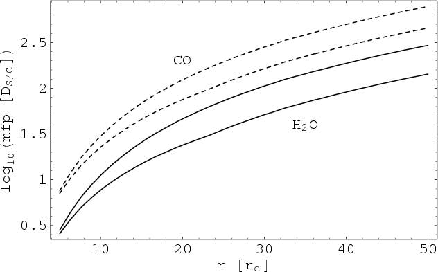
Figure 10 shows the computed m.f.p. on the subsolar axis at rotation phase
.
To estimate the inaccuracy of this, we
have played with this lower-limit.
Figure 10 shows the computed m.f.p. on the subsolar axis at rotation phase ![]() for two values of
for two values of
![]() .
We see that the maximum uncertainty is of a factor of 5.
.
We see that the maximum uncertainty is of a factor of 5.
|
Figure 10:
``Pseudo'' mean free paths for water (solid lines) and CO (dashed lines) are shown, expressed
in multiples of the characteristic orbiter size
|
| Open with DEXTER | |
5 Properties of the computed pressure field
5.1 Validity of the free-molecular spacecraft-gas interaction model
An essential assumption made in the preceding evaluation of the pressure force is that the spacecraft is submitted to a molecular flux given by the unperturbed coma gas flow velocity distribution. It can be shown that this requires thatHere, the worst case occurs with the smallest values of ![]() .
This would lead to
a restriction of our treatment to cometocentric distances larger than about
.
This would lead to
a restriction of our treatment to cometocentric distances larger than about
![]() .
That is, below
this altitude and given the supersonic relative spacecraft-gas motion, the gas-spacecraft interaction
occurs via the formation of a shock wave (attached or detached) in front of the spacecraft. The
latter is submitted to the pressure force of the shocked gas, hence its computation first requires
that of the shock structure.
.
That is, below
this altitude and given the supersonic relative spacecraft-gas motion, the gas-spacecraft interaction
occurs via the formation of a shock wave (attached or detached) in front of the spacecraft. The
latter is submitted to the pressure force of the shocked gas, hence its computation first requires
that of the shock structure.
5.2 Range of validity of the hypersonic approximation
For the present conditions where CO is dominant, ![]() is close to the
vibrationally relaxed CO value 1.4, hence
s = 0.84 M from Eq. (9), and
the condition
is close to the
vibrationally relaxed CO value 1.4, hence
s = 0.84 M from Eq. (9), and
the condition ![]() is equivalent to
is equivalent to ![]() .
Figure 9 indicates that this condition is always met
beyond 10 km (
.
Figure 9 indicates that this condition is always met
beyond 10 km (
![]() )
and never met at r < 5 km (
)
and never met at r < 5 km (
![]() ). Let us note that these distances
do not depend much upon the gas density, but depend strongly upon the nucleus shape and size.
). Let us note that these distances
do not depend much upon the gas density, but depend strongly upon the nucleus shape and size.
5.3 Spatial structure of the pressure field
Now we return to the important prefactor
![]() of Eq. (30). First one should
note that for the unphysical case of a spherical nucleus with homogeneous sublimation properties across
its surface, the prefactor is not dependent on the probe's longitude
of Eq. (30). First one should
note that for the unphysical case of a spherical nucleus with homogeneous sublimation properties across
its surface, the prefactor is not dependent on the probe's longitude ![]() in the cometocentric solar plane-of-sky (plane through the comet center, normal to the direction of the Sun).
If this property also holds for the adopted nucleus of irregular shape, then the contours on which the prefactor
is constant should be nearly horizontal in
in the cometocentric solar plane-of-sky (plane through the comet center, normal to the direction of the Sun).
If this property also holds for the adopted nucleus of irregular shape, then the contours on which the prefactor
is constant should be nearly horizontal in ![]() -
-![]() space, where
space, where ![]() is the angle between
the cometocentric direction of the spacecraft and the cometocentric direction of the Sun. We also want to
test if the pressure field drops as the inverse square of the distance r from some center of the comet.
If so, the function
is the angle between
the cometocentric direction of the spacecraft and the cometocentric direction of the Sun. We also want to
test if the pressure field drops as the inverse square of the distance r from some center of the comet.
If so, the function

should be fairly independent of r. The prefactor
In Fig. 11 the isocontours of ![]() are plotted in
are plotted in ![]() -
-![]() space for the initial
rotational phase of the nucleus, where
space for the initial
rotational phase of the nucleus, where ![]() is measured in the solar plane-of-sky, relative to the plane
which contains both the rotation axis and the cometocentric direction vector of the Sun. The different types
of curves represent different cometocentric distances of the spacecraft: r=10 (dashed), 25 (solid)
and
is measured in the solar plane-of-sky, relative to the plane
which contains both the rotation axis and the cometocentric direction vector of the Sun. The different types
of curves represent different cometocentric distances of the spacecraft: r=10 (dashed), 25 (solid)
and
![]() (densely dotted).
(densely dotted).

|
Figure 11:
The contours in |
| Open with DEXTER | |
From the figure we can infer three important properties of the pressure field. First of all, near
![]() the strength of the acceleration is
the strength of the acceleration is ![]()
![]() ,
which is comparable to the gravitational acceleration generated by the comet
,
which is comparable to the gravitational acceleration generated by the comet
|
(47) |
with a nominal nucleus mass of
Third, the contour types (solid, dashed, densely dotted) representing
different cometocentric distances overlap fairly well. In other words,
the outgassing pressure field drops roughly as the inverse square
distance from some center of the nucleus. From the figure one can see
that this property begins to degrade as r decreases, but studies show that important structures are still preserved as close to the nucleus as
![]() .
This means that we can approximate the pressure field, or more precisely
.
This means that we can approximate the pressure field, or more precisely
![]() ,
by Fourier expansions in
,
by Fourier expansions in ![]() and
and ![]() ,
if not too close to the comet's nucleus (
,
if not too close to the comet's nucleus (
![]() ). However, Fig. 11 demonstrates that such Fourier expansions will be of a relatively high order due to the large degree of variability of
). However, Fig. 11 demonstrates that such Fourier expansions will be of a relatively high order due to the large degree of variability of ![]() .
Also, the coefficients of the expansions will clearly exhibit large temporal variations as the nucleus rotates.
.
Also, the coefficients of the expansions will clearly exhibit large temporal variations as the nucleus rotates.
5.4 Variability
This is shown explicitly in Fig. 12 where isocontours of
![]() are mapped over a rotation period.
are mapped over a rotation period.

|
Figure 12:
The isocontours of the amplitude
|
| Open with DEXTER | |

|
Figure 13:
The variation of |
| Open with DEXTER | |
However, if the outgassing pressure perturbation of the spacecraft's Keplerian motion is sufficiently weakened by a minimized exposure of the probe's arrays, it follows from first-order perturbation theory that the mean motion of the orbit, and therefore also the Doppler observable, can be characterized by a time-averaged pressure field. This way, a systematic drift of the Doppler observable related to the non-periodic evolution of the spacecraft's cometocentric orbit can be accounted for over a limited time-scale. It should be stressed though that the Doppler signal related to the short-periodic (similar to rotation period of nucleus) variations of the orbit, induced by the outgassing pressure, are not accounted for in a mean field approximation. So the variations which are not accounted for can mask the Doppler signal related to the second degree and order gravity field of the nucleus. Still, to determine the nucleus oblateness (second degree, zero order gravity field), nucleus mass and position of the spacecraft relative to the nucleus, it is a proper description of the mean pressure field which is important, but only if it can be viewed as a weak perturbation.
5.5 Mean field
We will return to these topics later on in this paper, but before doing
so, some properties of the mean outgassing pressure field
![]() (strictly speaking not the pressure field, but the spacecraft's response to the pressure field) based on Eq. (46)
will be quantified. The isocontours of the time-averaged field with
equal weight on the 72 available rotational phases of the comet
nucleus are shown in Fig. 14. The different types of curves represent the cometocentric distances r=10 (dashed), 25 (solid), and
(strictly speaking not the pressure field, but the spacecraft's response to the pressure field) based on Eq. (46)
will be quantified. The isocontours of the time-averaged field with
equal weight on the 72 available rotational phases of the comet
nucleus are shown in Fig. 14. The different types of curves represent the cometocentric distances r=10 (dashed), 25 (solid), and
![]() (densely dotted). From plots like Fig. 11 we already know that
(densely dotted). From plots like Fig. 11 we already know that
![]() will be fairly independent of distance r, but Fig. 14 shows that this property is slightly improved.
will be fairly independent of distance r, but Fig. 14 shows that this property is slightly improved.

|
Figure 14:
The curves on which the time averaged pressure field
|
| Open with DEXTER | |
As one would perhaps expect, this mean field is more well-behaved than the instantaneous ones of Fig. 11. In order to quantify this property, we have fitted
![]() to expansions in spherical harmonic functions (Kaula 2000) of the order N
to expansions in spherical harmonic functions (Kaula 2000) of the order N

by the least-squares method. Above,

|
(49) |
is a normalization factor so that the values of

defined on a

will also be of interest.
Accordingly, we see that if we define
![]() due to the approximate symmetry of Fig. 14, a truncation at N=3 of Eq. (48) represents a good balance between keeping N low on one side and
due to the approximate symmetry of Fig. 14, a truncation at N=3 of Eq. (48) represents a good balance between keeping N low on one side and ![]() and
and
![]() small on the other,
Table 2.
small on the other,
Table 2.
Table 2:
Fit adequacy parameter
![]() (and
(and
![]() )
for an N=3 expansion Eq. (48) fitted to
)
for an N=3 expansion Eq. (48) fitted to
![]() ).
).
Table 3:
Coefficients
![]() of an expansion in spherical harmonics fitted to
of an expansion in spherical harmonics fitted to
![]() of Eq. (46).
of Eq. (46).
Of course, whether or not the approximation
![]() is valid for a real nucleus is highly uncertain. For instance, the
outgassing across the nucleus surface may be highly dependent on the
different types of nucleus ices and the location of the nucleus
sublimation fronts, and the mean field may therefore have other
directions of preference than that of the Sun and the nucleus rotation
axis.
is valid for a real nucleus is highly uncertain. For instance, the
outgassing across the nucleus surface may be highly dependent on the
different types of nucleus ices and the location of the nucleus
sublimation fronts, and the mean field may therefore have other
directions of preference than that of the Sun and the nucleus rotation
axis.
In order to obtain the same quality of the fit for the instantaneous field of
Fig. 11 as of Table 2, the order of the expansion in spherical harmonics must be carried out up to and including order N=10.
This means that by adopting the mean field approach and thereby
neglecting the outgassing induced short-period variations of the
Doppler signal the number of parameters is reduced from more than
121 ( N=10) to
![]() .
.
5.6 The expansion velocity
From Eq. (37) we see that the drift velocity V
of the outgassing pressure field is important if the incident gas
molecules are thermalized by the spacecraft walls. From plots of
the V in ![]() -
-![]() space for different rotational phases one can see that the structures
of the field are non-trivial, but this time the field's variability in
the angles is significantly reduced. This is clearly illustrated in
Fig. 15 where
space for different rotational phases one can see that the structures
of the field are non-trivial, but this time the field's variability in
the angles is significantly reduced. This is clearly illustrated in
Fig. 15 where
![]() over the 72 rotational phases (one rotation period) are plotted at the distance
over the 72 rotational phases (one rotation period) are plotted at the distance
![]() and should be compared to a global mean of
and should be compared to a global mean of
![]() .
.

|
Figure 15:
The isocontours of the velocity amplitude over a rotation period are plotted above. Here the curves with the values
|
| Open with DEXTER | |
Also, the simulations show that V is fairly independent of r beyond some distance. To quantify this property, we have again fitted simplified expansions like the one of
Eq. (48) to the mean velocity field
![]() ,
calculated from the 72 available phases. Using the criteria Eqs. (50) and (51), and the simple expression
,
calculated from the 72 available phases. Using the criteria Eqs. (50) and (51), and the simple expression
![\begin{displaymath}
\overline{V}\approx{}[~635+142~\cos\theta~]~{\rm m}~{\rm s}^{-1},
\end{displaymath}](/articles/aa/full_html/2010/04/aa12107-09/img285.png)
we obtain the acceptable results of Table 4.
Table 4:
Fit parameter
![]() (and
(and
![]() )
for the expression Eq. (52), calculated as a least-squares approximation to
)
for the expression Eq. (52), calculated as a least-squares approximation to
![]() ).
).
6 Applications
6.1 Mean field model
The purpose of a mean field model like Table 2 is that it can be used to reduce the difference between observed and computed data during a comet rendezvous mission. If the differences, also called residuals, are similar to the observation noise, we can say that we have an adequate description of reality.
As for Rosetta, one essential data type for the radio science
objectives, like the determination of the comet nucleus' gravity field,
are Doppler data with an observation noise of
![]() for long integration times (Pätzold et al. 2007). Below we shall use the cometocentric velocity component
for long integration times (Pätzold et al. 2007). Below we shall use the cometocentric velocity component ![]() of the spacecraft in the direction of the Sun as the Doppler
observable, an acceptable approximation since the cometocentric
direction of the Earth approximately coincides with that of the Sun at
the early stages of the Rosetta mission (Mysen & Aksnes 2008). The
unit vector
of the spacecraft in the direction of the Sun as the Doppler
observable, an acceptable approximation since the cometocentric
direction of the Earth approximately coincides with that of the Sun at
the early stages of the Rosetta mission (Mysen & Aksnes 2008). The
unit vector ![]() ,
which describes the velocity direction of the spacecraft relative to the atmosphere is set to
,
which describes the velocity direction of the spacecraft relative to the atmosphere is set to
![]() .
.
In Fig. 16 the difference
![]() between ``real'' Doppler data, generated using the full coma simulations, and the mean field model Table 2, is shown as the solid line. Three important initial orbit elements are the cometocentric semi-major axis
between ``real'' Doppler data, generated using the full coma simulations, and the mean field model Table 2, is shown as the solid line. Three important initial orbit elements are the cometocentric semi-major axis
![]() (initial orbit period of 560 h), the eccentricity e0=0.2 and the orbit's inclination with respect to the cometocentric solar plane-of-sky I0=0.5.
The choice of a small inclination value is motivated by stability
reasons. So if the orbit is to remain bound for the duration of the
studied time interval of
(initial orbit period of 560 h), the eccentricity e0=0.2 and the orbit's inclination with respect to the cometocentric solar plane-of-sky I0=0.5.
The choice of a small inclination value is motivated by stability
reasons. So if the orbit is to remain bound for the duration of the
studied time interval of
![]() ,
then the surface of Rosetta exposed to outgassing has to be minimized, see Figs. 4 and 5.
Still, the spacecraft's cometocentric orbit elements are seen to
undergo significant changes over the time span shown in the plot.
Radiation pressure from the Sun is very important, but is nevertheless
not included since we choose to focus solely on the properties of the
pressure forces due to outgassing from the comet nucleus.
,
then the surface of Rosetta exposed to outgassing has to be minimized, see Figs. 4 and 5.
Still, the spacecraft's cometocentric orbit elements are seen to
undergo significant changes over the time span shown in the plot.
Radiation pressure from the Sun is very important, but is nevertheless
not included since we choose to focus solely on the properties of the
pressure forces due to outgassing from the comet nucleus.
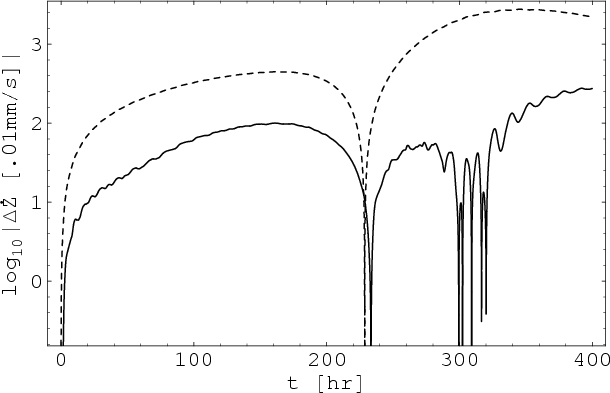
|
Figure 16: The differences between ``real'' Doppler data from a cometary orbiter, generated using the full coma simulations, and model calculations are shown. For the dashed curve, the applied model is pure Kepler motion. The solid line is produced using the mean field of Table 2 as model. The dips in the lines are due to crossings between the ``real'' Doppler data and those simulated by the different models (Kepler, mean field). |
| Open with DEXTER | |
Although the mean field model reduces the residuals in comparison to a
model which only includes Kepler motion as represented by the dashed
line in Fig. 16,
the resulting residuals are far from similar to one, as should be
required for a proper description of reality of this maximum CO
production scenario. When the
![]() coefficients of the mean field model are fitted to real Rosetta data in
2014, the residuals will become smaller than those of Fig. 16, provided that the prerequisites for the coma simulations and reality are the same. However, the solve for coefficients
coefficients of the mean field model are fitted to real Rosetta data in
2014, the residuals will become smaller than those of Fig. 16, provided that the prerequisites for the coma simulations and reality are the same. However, the solve for coefficients
![]() will then not represent the global field as those of Table 2, but the local pressure forces in parts of the coma which the probe has traversed.
will then not represent the global field as those of Table 2, but the local pressure forces in parts of the coma which the probe has traversed.
The mean field approach is improved as the probe's distance to the comet increases.
6.2 Determination of gravity field
As previously mentioned, a stated goal of the Rosetta Radio Science
Investigations is the determination of the nucleus' gravity field from
Doppler data (Pätzold et al. 2007). The cometocentric
gravitational acceleration
![]() of an orbiting spacecraft can be obtained by taking the gradient of the gravitational potential
of an orbiting spacecraft can be obtained by taking the gradient of the gravitational potential
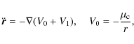
where
![\begin{displaymath}
V_1=\frac{\mu_{\rm c}}{r}~\left(\frac{r_{\rm c}}{r}\right)^2...
...P_{20}(\sin\beta)+c_{22}P_{22}(\sin\beta)\cos2\lambda~\right].
\end{displaymath}](/articles/aa/full_html/2010/04/aa12107-09/img297.png)
Here, P2m are Legendre functions, and
6.2.1 Nucleus oblateness
The Doppler signals related to the two latter parameters are mainly experienced through variations
in the probe's cometocentric velocity component in the direction of the observer (Mysen & Aksnes 2008),
![]() .
To investigate whether or not these gravity induced variations are drowned
in the corresponding variations induced by outgassing pressure, we have mapped the difference
.
To investigate whether or not these gravity induced variations are drowned
in the corresponding variations induced by outgassing pressure, we have mapped the difference

|
(55) |
where the first component is generated using Kepler acceleration and the full outgassing pressure model (solid curve of Fig. 17), or Kepler acceleration and the oblateness parameter c20=0.088 (arbitrary choice) of Eq. (54) (dashed curve of Fig. 17). From the simulations we found that the the outgassing pressure prefactor

|
Figure 17:
Doppler signals related to the outgassing pressure (solid) and the nucleus' c20 gravity field (dashed) are shown for an initial orbit semi-major axis of
|
| Open with DEXTER | |

|
Figure 18:
The oscillations of the Doppler signals related to the short-periodic
variations of the outgassing pressure field (solid) and the c22
gravity field (dashed) are shown as the spacecraft travels through the
night side of the coma, with an initial orbit semi-major axis
|
| Open with DEXTER | |
If we make the conservative assumption that we have no a priori
knowledge of the properties of the coma, i.e., that realistic coma
simulations are not available, we can see that the signal related to c20 begins to become discernible at the cometocentric distance
![]() of Fig. 17. Above this height, the component is drowned in the outgassing signal since the acceleration due to this gravity term drops as
of Fig. 17. Above this height, the component is drowned in the outgassing signal since the acceleration due to this gravity term drops as ![]() r-4, while the outgassing induced acceleration diminishes as
r-4, while the outgassing induced acceleration diminishes as ![]() r-2. That is, the amplitude of the periodic variations induced by a perturbing acceleration
r-2. That is, the amplitude of the periodic variations induced by a perturbing acceleration
![]() ,
with a frequency equal to the orbit frequency
,
with a frequency equal to the orbit frequency
![]() ,
can be approximated by the expression
,
can be approximated by the expression

where f is the true anomaly of the spacecraft in its orbit, and

|
(57) |
where
6.2.2 Nucleus triaxiality
As for the
![]() (arbitrary choice) gravity coefficient related to the nucleus' triaxiality, we have studied the velocity differences
(arbitrary choice) gravity coefficient related to the nucleus' triaxiality, we have studied the velocity differences

|
(58) |
to see if one can discern the c22 induced variations. We compared the difference in the Doppler signal between a full outgassing model and the mean outgassing model (solid curve of Fig. 18) to the result when the full model is extended to include the c22 component (dashed curve of Fig. 18). Again, the pressure field prefactor
From a similar approach as that of Eq. (56), we derive the amplitude of the oscillations of Fig. 18 as

|
(59) |
where
where
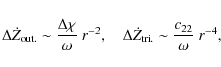
It is important to note that the outgassing induced variations of the
Doppler signal, with a period similar to the rotation period of the
nucleus, and the estimated amplitude given by Eq. (60) cannot be removed from the data by the mean field approach of Eq. (48). According to Eq. (60),
the amplitude of these outgassing induced Doppler signal variations are
several orders of magnitude larger than the Doppler observation noise
in the day side of the coma at cometocentric distance
![]() .
Consequently the mean field model alone is not an adequate description
of reality in general during the Rosetta mission for the presented
maximum CO production scenario. However, as already shown in
Fig. 18,
at the same distance and in the night side of the coma, the outgassing
induced variations of the Doppler signal are comparable to the Doppler
noise, if the CO pressure field is down-scaled one order of
magnitude in comparison to the maximum production scenario.
.
Consequently the mean field model alone is not an adequate description
of reality in general during the Rosetta mission for the presented
maximum CO production scenario. However, as already shown in
Fig. 18,
at the same distance and in the night side of the coma, the outgassing
induced variations of the Doppler signal are comparable to the Doppler
noise, if the CO pressure field is down-scaled one order of
magnitude in comparison to the maximum production scenario.
7 Discussion
In support of navigation and radio science during ESA's Rosetta mission, we have reviewed a simple model for the interaction between a spacecraft and a Maxwellian atmosphere and applied it to the Rosetta spacecraft with some simplifying assumptions with respect to its outer shape, molecular scattering properties, and temperature.
A state-of-the-art 3D+t gasdynamical simulation of the coma around the irregularly shaped nucleus of 67P was used to analyze the interaction. The simulation parameters are selected to yield upper-limit 3 AU total production rates of water - by solar-driven sublimation - and of CO (which dominates at this heliocentric distance). The production of CO was assumed to be moderately uneven over the surface, giving birth to a moderately contrasted pressure field, in comparison with what would have been obtained if the production had been assumed concentrated in a localized area of the nucleus. The spatial resolution of the model was three degrees in longitude and latitude, and the time resolution was 1/72 of the rotation period.
The present results have only been established for probe distances between 5 and 50 mean comet radii.
First of all, it was found that the probe distance to the nucleus must be larger than 5-10 mean comet radii if the mean free path of the molecules in the cometocentric direction of the Sun is to be much larger than the size of the spacecraft. Below this distance, one may need to include the spacecraft as part of the coma simulation to obtain reliable results.
It was also found that the pressure force may be dependent on the coma temperature in the night-side of the coma, and that beyond about 5-10 mean comet radii outwards, the gas flow direction was mainly directed away from the nucleus.
We found that the pressure force on Rosetta is amplified by a non-zero spacecraft temperature and that the force does not act mainly away from the comet nucleus in general. Three parameters were suggested to describe the interaction, assuming that one type of molecule is the main contributor to the pressure.
For probe orbit sizes above 5-10 mean comet radii, the pressure field was seen to drop as the inverse square of the distance to the comet nucleus. This separability of the pressure field dependency in probe direction and probe distance simplifies the search for representative pressure field models. However, the force field is significantly distorted due to the non-spherical shape of the comet nucleus. As a result, deterministic models which aim to represent the properties of the instantaneous coma will contain too many parameters and will therefore not be practical.
The average pressure field over a nucleus rotation period, on the other hand, was seen to be well represented by a relatively small number of parameters. However, for the ``nearly maximum'' gas production scenario studied, it was established that this mean field model alone was not able to describe reality to sufficient precision during the Rosetta mission.
In the general direction of the Sun, the maximum drag force on Rosetta was seen to be larger than the gravitational attraction from the nucleus at all probe distances.
As for the determination of the gravity field coefficients related to the nucleus oblateness and triaxiality through Doppler data, it was seen that it was easier to discern the latter from the ``noise'' induced by outgassing pressure forces on Rosetta. The reason for this is that the Doppler signature of the nucleus triaxiality is resolved over a shorter time interval compared to that of the nucleus oblateness. As a result, the nucleus triaxiality can be determined in a limited region of the coma where the variability of the outgassing pressure field, or ``noise'', is small. The Doppler signal related to the nucleus oblateness is, on the other hand, only resolved on a time scale similar to that of the spacecraft's orbit period. During this time scale, the probe will have experienced the global, and not only local, properties of the coma. If the nucleus rotation is not uniaxial as assumed above, the gravity field related to the nucleus oblateness could also be discernible on a time scale similar to the nucleus rotation period (Mysen et al. 2006).
As similar state-of-the-art coma simulations based on Rosetta observations will be available in 2014-2015, it should to a large extent be possible to remove the signal related to outgassing pressure forces from Doppler data. As a result, it should be easier to determine the gravity field coefficients of the nucleus.
It should be noted that in case the rotation of the target nucleus is not found to be uniaxial, the nucleus rotation will nevertheless be approximately periodic (also called quasi-periodic) on a limited time scale. Coma simulations can then be executed covering nucleus rotation phases over this approximate rotation period.
AcknowledgementsThis work was possible due to supports from the Research Council of Norway, project 184686, and, in France, from the CNES ``Rosetta Croisière'' funding.
References
- Byram, S. M., Scheeres, D. J., & Combi, M. R. 2007, J. Guid. Cont. Dyn., 30, 5, 1445 [Google Scholar]
- Capria, M. T., Coradini, A., De Sanctis, M. C., & Fulle, M. 2004, in The New ROSETTA Targets, ed. L. Colangeli, E. M. Epifani, & P. Palumbo (Dordrecht: Kluwer), ASSL, 311, 177 [Google Scholar]
- Crifo, J. F. 1995, A&A, 300, 597 [NASA ADS] [Google Scholar]
- Crifo, J. F. 2006, Adv. Space Res., 38, 1911 [NASA ADS] [CrossRef] [Google Scholar]
- Crifo, J. F., Rodionov, A. V., Szegö, K., & Fulle, M. 2002, Earth, Moon and Planets, 90, 227 [Google Scholar]
- Crifo, J. F., Fulle, M., Kömle, N. I., & Szegö, K. 2004a, in Comets II, ed. M. C. Festou, H. U. Keller, & H. A. Weaver (Tucson: The University of Arizona Press), 471 [Google Scholar]
- Crifo, J. F., Lukyanov, G. A., Zakharov, V. V., & Rodionov, A. V. 2004b, in The New ROSETTA Targets, ed. L. Colangeli, E. M. Epifani, & P. Palumbo (Dordrecht: Kluwer), ASSL, 311, 119 [Google Scholar]
- Davidsson, B. J. R., & Gutiérrez, P. J. 2005, Icarus, 176, 453 [NASA ADS] [CrossRef] [Google Scholar]
- Feaga, L. M., A'Hearn, M. F., Sunshine, J. M., Groussin, O., & Farnham, T. L. 2007, Icarus, 190, 345 [NASA ADS] [CrossRef] [Google Scholar]
- Harrison, I. K., & Swinerd, G. G. 1996, Planet. Space Sci., 44, 2, 171 [CrossRef] [Google Scholar]
- Kaula, W. M. 2000, Theory of Satellite Geodesy (New York: Dover Publications) [Google Scholar]
- Lamy, P. L., Toth, I., Davidsson, B. J. R., et al. 2007, Space Sci. Rev., 128, 23 [NASA ADS] [CrossRef] [Google Scholar]
- Moe, K., & Moe, M. M. 2005, Planet. Space Sci., 53, 793 [NASA ADS] [CrossRef] [Google Scholar]
- Moore, P., & Sowter, A. 1991, Planet. Space Sci., 39, 10, 1405 [Google Scholar]
- Mysen, E., & Aksnes, K. 2006, A&A, 455, 1143 [NASA ADS] [CrossRef] [EDP Sciences] [Google Scholar]
- Mysen, E., & Aksnes, K. 2008, A&A, 490, 447 [NASA ADS] [CrossRef] [EDP Sciences] [Google Scholar]
- Mysen, E., Olsen, Ø, & Aksnes, K. 2006, Planet. Space Sci., 54, 750 [NASA ADS] [CrossRef] [Google Scholar]
- Pätzold, M., Häusler, B., Aksnes, K., et al. 2007, Space Sci. Rev., 128, 599 [NASA ADS] [CrossRef] [Google Scholar]
- Prialnik, D.,Benkhoff, J., & Podolak, M., in Comets II, ed. M. C. Festou, H. U. Keller, & H. A. Weaver (Tucson: The University of Arizona Press), 359 [Google Scholar]
- Rodionov, A. V., & Crifo, J. F. 2006, Adv. Space Res., 38, 1923 [NASA ADS] [CrossRef] [Google Scholar]
- Rodionov, A. V., Crifo, J. F., Szegö, K., Lagerros, J., & Fulle, M. 2002, Planet. Space Sci., 50, 983 [NASA ADS] [CrossRef] [Google Scholar]
- Scheeres, D. J., Bhargava, S., & Enzian, A. 2000, A Navigation Model of the Continuous Outgassing Field Around a Comet, TMO Progress Report 42 [Google Scholar]
- Valorge, C. 1995, in Spaceflight Dynamics Part I, ed. J.-P. Carrou, CNES, 217 [Google Scholar]
- Weeks, C. J. 1995, J. Astronaut. Sci., 43, 3, 327 [Google Scholar]
- Zakharov, V. V., Rodionov, A. V., Lukyanov, G. A., & Crifo, J.-F. 2008, Icarus 194, 327 [CrossRef] [Google Scholar]
All Tables
Table 1: Comet 67P model parameters.
Table 2:
Fit adequacy parameter
![]() (and
(and
![]() )
for an N=3 expansion Eq. (48) fitted to
)
for an N=3 expansion Eq. (48) fitted to
![]() ).
).
Table 3:
Coefficients
![]() of an expansion in spherical harmonics fitted to
of an expansion in spherical harmonics fitted to
![]() of Eq. (46).
of Eq. (46).
Table 4:
Fit parameter
![]() (and
(and
![]() )
for the expression Eq. (52), calculated as a least-squares approximation to
)
for the expression Eq. (52), calculated as a least-squares approximation to
![]() ).
).
All Figures
|
|
Figure 1:
A flat plate is seen from its side.
The plate moves with a velocity |
| Open with DEXTER | |
| In the text | |
|
|
Figure 2:
The pressure force coefficient CV of Eq. (21) is given for different values of s, dashed lines. From bottom to top we have s=1, s=3, and
|
| Open with DEXTER | |
| In the text | |
|
|
Figure 3:
From bottom to top, |
| Open with DEXTER | |
| In the text | |
|
|
Figure 4:
The figure illustrates effective areas of Rosetta in the drag
direction: total (solid), without bus (dotted), or with the spacecraft
temperature set to
|
| Open with DEXTER | |
| In the text | |
|
|
Figure 5:
The lift to drag ratio is shown above as a function of the attack angle |
| Open with DEXTER | |
| In the text | |
| |
Figure 6: Present best-fit shape of the comet 67P nucleus. The largest diameter is about 5 km. The uncertainty is probably on the order of the magnitude of the topographic features. The corresponding best-fit monoaxial rotation is about the z-axis. The model will be periodically improved as new observational data are accumulated. After Lamy et al. (2007). |
| Open with DEXTER | |
| In the text | |
|
|
Figure 7: Variation of the total mass density in the equatorial plane during the rotation. From left to right and from top to bottom: isocontours of Log10 (mass density, kg/m3) in the equatorial plane are shown every 1/9 of the rotation period (i.e., every 1.4 h.) The projected Sun direction is to the right. Notice the clockwise rotation of the nucleus cross section. On this and the two next figures, references and dates appear at the bottom left of each panel for safety of identification: the reader must overlook them. The dust contribution has not been included. |
| Open with DEXTER | |
| In the text | |
|
|
Figure 8: Log10 of the H2O ( upper panels) and CO ( lower panels) density in two orthogonal planes at rotation phase 0. The projected Sun direction is to the right on the X-axis ( right panels) or at 200 to the X-axis ( left panels). The total density shown on Fig. 7 ( upper left panel) is the sum of the two present right panel densities. |
| Open with DEXTER | |
| In the text | |
|
|
Figure 9: Velocity ( upper panels) and Mach number ( lower panels) in two orthogonal planes at rotation phase 0. The projected Sun direction is to the right on the X-axis ( right panels) or at 200 to the X-axis ( left panels). |
| Open with DEXTER | |
| In the text | |
|
|
Figure 10:
``Pseudo'' mean free paths for water (solid lines) and CO (dashed lines) are shown, expressed
in multiples of the characteristic orbiter size
|
| Open with DEXTER | |
| In the text | |
|
|
Figure 11:
The contours in |
| Open with DEXTER | |
| In the text | |
|
|
Figure 12:
The isocontours of the amplitude
|
| Open with DEXTER | |
| In the text | |
|
|
Figure 13:
The variation of |
| Open with DEXTER | |
| In the text | |
|
|
Figure 14:
The curves on which the time averaged pressure field
|
| Open with DEXTER | |
| In the text | |
|
|
Figure 15:
The isocontours of the velocity amplitude over a rotation period are plotted above. Here the curves with the values
|
| Open with DEXTER | |
| In the text | |
|
|
Figure 16: The differences between ``real'' Doppler data from a cometary orbiter, generated using the full coma simulations, and model calculations are shown. For the dashed curve, the applied model is pure Kepler motion. The solid line is produced using the mean field of Table 2 as model. The dips in the lines are due to crossings between the ``real'' Doppler data and those simulated by the different models (Kepler, mean field). |
| Open with DEXTER | |
| In the text | |
|
|
Figure 17:
Doppler signals related to the outgassing pressure (solid) and the nucleus' c20 gravity field (dashed) are shown for an initial orbit semi-major axis of
|
| Open with DEXTER | |
| In the text | |
|
|
Figure 18:
The oscillations of the Doppler signals related to the short-periodic
variations of the outgassing pressure field (solid) and the c22
gravity field (dashed) are shown as the spacecraft travels through the
night side of the coma, with an initial orbit semi-major axis
|
| Open with DEXTER | |
| In the text | |
Copyright ESO 2010
Current usage metrics show cumulative count of Article Views (full-text article views including HTML views, PDF and ePub downloads, according to the available data) and Abstracts Views on Vision4Press platform.
Data correspond to usage on the plateform after 2015. The current usage metrics is available 48-96 hours after online publication and is updated daily on week days.
Initial download of the metrics may take a while.