Photometric survey of the very small near-Earth asteroids with the SALT telescope - III. Lightcurves and periods for 12 objects and negative detections

T. Kwiatkowski; M. Polinska; N. Loaring; D. A. H. Buckley; D. O'Donoghue; A. Kniazev; E. Romero Colmenero

doi:10.1051/0004-6361/200913468

Home

All issues

Volume 511 (February 2010)

A&A, 511 (2010) A49

Full HTML

Free Access

Issue		A&A Volume 511, February 2010


Article Number		A49
Number of page(s)		10
Section		Planets and planetary systems
DOI		https://doi.org/10.1051/0004-6361/200913468
Published online		09 March 2010

A&A 511, A49 (2010)

Photometric survey of the very small near-Earth asteroids with the SALT telescope^,

III. Lightcurves and periods for 12 objects and negative detections

T. Kwiatkowski¹ - M. Polinska¹ - N. Loaring² - D. A. H. Buckley² - D. O'Donoghue² - A. Kniazev² - E. Romero Colmenero²

1 - Astronomical Observatory, Adam Mickiewicz University, S $\l$ oneczna 36, 60-286 Poznan, Poland
2 - South African Astronomical Observatory, Observatory Road, Observatory 7925, South Africa

Received 14 October 2009 / Accepted 24 November 2009

Abstract
Aims. Very small asteroids (VSAs) are thought to be the building blocks of larger asteroids and, as such, are interesting to study. Many of these monolithic or deeply fractured objects display rapid rotations with periods as short as several minutes. Observations of such asteroids can reveal their spin limits, which can be related to the tensile strength of their interiors. The evolution of the spins of these objects is primarily shaped by the YORP effect, the theory of which needs comparison with observations.
Methods. With the 10 m SALT telescope, we observed VSAs belonging to near-Earth asteroids. The obtained lightcurves were used to derive synodical periods of rotation, amplitudes, and elongations of these bodies.
Results. Results for 14 rapidly rotating asteroids were reported in the first paper in this series. Here we show lightcurves of 2 fast rotators, 9 objects with periods $\geq$ 1 h, and a possible non-principal axis rotator. We also list negative detections that most probably indicate asteroids with long periods and/or low amplitudes. Combining our results with the data from the literature, we obtain a set of 79 near-Earth VSAs with a median period of 0.25 h (15 min). By adjusting the spin limits predicted by theory to those observations, we find tentative evidence that the tensile strengths of VSAs, after scaling them to the same size, are of the same order as the minimum tensile strengths of stony meteoroids that undergo fragmentation under the atmospheric load.

Key words: techniques: photometric - minor planets, asteroids: general

1 Introduction

This is the third paper in the series reporting the results of the extensive photometric survey of very small near-Earth asteroids, performed with the 10 m Southern African Large Telescope (SALT). By very small asteroids (VSAs) we are referring to objects with absolute magnitudes H>21.5 mag, which translates to effective diameters smaller than D=0.15 km (with the assumed geometric albedo $p_{{\rm V}}=0.20$ - see Warner et al. 2009 for justification of this value). Due to their faintness, most of them are observed as near-Earth asteroids (hereafter NEAs), but there are also several VSAs from the Main Belt, whose reliable periods have been derived.

The instruments and the methods of data reduction were described in Kwiatkowski et al. (2009), which presents observations of an unusual asteroid 2006 RH₁₂₀. A systematic presentation of the early results of the survey was presented in Kwiatkowski et al. (2010) (hereafter Paper I) where we published the lightcurves of a sample of the fastest rotating asteroids (periods shorter than 1 h). We described the selection criteria and presented the rotation periods, amplitudes and elongations for 14 objects.

In the second paper (Paper II, Kwiatkowski 2010), we discussed future close approaches of the observed fast-rotators (adding the objects already studied before), as well as the possibility of detecting the YORP effect from their rotation periods. We also constrained the pole position of 2006 XY, whose spin axis obliquity was found to be smaller than $50\hbox{$^\circ$ }$ .

In the present paper we report another 12 objects observed during our survey: 2 asteroids with periods shorter than 1 h, 9 objects with periods of 1-4.5 h, as well as a possible non-principal axis rotator. We also mention negative detections of asteroids, for which no brightness changes were observed above our level of detection. At the end we combine our results with the existing database of rotation periods of VSAs and compare them with spin limits predicted by theory.

Table 1: Aspect data and the observing log.

2 Lightcurves of 12 asteroids

In this section we present observations and derive periods and elongations of 12 asteroids from our survey. The synodic periods of most of them are found to be longer than 1 h, which made it difficult to observe all rotation phases with SALT. As explained in Paper I, SALT can usually observe targets twice a night, during the East and West tracks, each of which last about one hour. Due to this limitation, in the analysis we assume a typical two maxima, two minima lightcurve, which means there is ambiguity in the derived periods. Although unlikely, the true periods could be two times shorter or longer than the obtained results. Such uncertainties are typical in the case of many VSAs, and their periods can still be used for statistical analyzes. The aspect data and observing log for each asteroid are given in Table 1.

2.1 2007 CX₅₀

This Apollo asteroid was discovered by the Catalina Sky Survey on 15 Feb. 2007 and announced in Minor Planet Electronic Circular (hereafter MPEC) 2007-C71. We observed it with SALT on 17 Feb. under photometric conditions and on 19 Feb., under clear conditions. Unfortunately, on 19 Feb. the image quality (IQ) was poor, and to measure the images we had to use $12\hbox{$^{\prime\prime}$ }$ apertures (the aperture diameter used on 17 Feb. frames was only $6\hbox{$^{\prime\prime}$ }$ ). Additionally, we had to discard data from the beginning and the end of the track due to their increased noise.

The asteroid brightness was measured with with respect to one comparison star with five other check stars being used to monitor the instrumental effects (a similar procedure was used in the case of other objects reported in this paper). The scatter of the check stars was at the level of $\pm 0.05$ mag with occasional systematic shifts also present. Obviously, these effects can also be traced in the lightcurve of 2007 CX₅₀(Fig. 1). For example, at rotation phases of 0.1 and 0.25 the asteroid brightness drops by 0.1 mag which is an instrumental effect as it disturbs the continuity of the curve.

During the 17 Mar. observations the telescope had to be re-pointed in the middle of the track, which resulted in a new set of comparison stars being used. Unfortunately, none of them were the same as those used previously and so we could not obtain the exact magnitude shift between the two parts of the data. This situation also arose for other asteroids presented in this paper. The magnitude shifts in such cases were either derived during a least-square fit of the Fourier series or estimated by manually shifting parts of the data based on the overlapping parts of the fragmentary curves.

The lightcurve of 2007 CX₅₀ appears to have a period P > 1 h so we were unable to cover all phases of its rotation and had to assume a typical two maxima, two minima lightcurve to estimate the period. During the observations on 17 Feb. we recorded part of one shallow maximum (Max₁), and most of the other maximum (Max₂, Fig. 1). The maxima are separated by $\Delta t_{1} \approx 0.029$ d which is equivalent to about 0.5 P or, more conservatively, $0.4 P < \Delta t_{1} < 0.6 P$ . From this we obtain $P= 1.45 \pm 0.3$ h, where the quoted uncertainty is the maximal error rather than the standard deviation.

There is part of the lightcurve from the 19 Feb., which covers the whole maximum (Max₃). It is similar in shape to the maximum Max₂ from the 17th. We can identify the two as the same feature, separated by $\Delta t_{2}=1.993$ d. Unfortunately, the accuracy of our first approximation of P is insufficient to connect Max₃ and Max₂ without ambiguity. Using Eq. (3) in Paper I, or rather its modified version for the lightcurves with distinguishable maxima, we can see that to be able to fold both the 17th and the 19th maxima, we should first derive the period with an accuracy better than $0.5~ P^2 \Delta t_{2}^{-1}$ or 0.02 h. On the other hand, we can use the 19 Feb. data to reconstruct part of the lightcurve. Since Max₃corresponds to Max₂, we can fold them obtaining a wider coverage of this feature. Further we can shift the obtained lightcurve fragments so that the common parts of Max₁ and the combined Max₂ and Max₃ are superimposed (without Max₃ this would have been impossible). The result, presented in Fig. 1 is used to estimate the peak-to-peak amplitude of 2007 CX₅₀ as $A \geq 0.8$ mag. This in turn suggests an asteroid elongation of $a/b \geq 1.6$ .

$\begin{figure} \par\resizebox{9cm}{!}{\includegraphics[clip]{13468f01.eps}} \end{figure}$	Figure 1: Composite lightcurve of 2007 CX₅₀ obtained with a period P=1.45 h. The part of the Fourier fit beyond the 0.65 phase is unconstrained by the data and serves only as an example. The zero phase in this and the subsequent plots is corrected for light-time.
Open with DEXTER

2.2 2007 EO

Discovered on 9 Mar. 2007 by the Siding Spring Survey (MPEC 2007-E41), this Amor asteroid was observed with SALT on four nights: 12 (both East and West tracks), 15, 20, and 31 Mar. 2007. All of the nights were photometric except the 12 Mar., where there were scattered clouds in the sky. On 31 Mar. observations were taken in bright time, which resulted in increased noise in the asteroid's brightness. The images were measured with apertures of $5\hbox{$^{\prime\prime}$ }, 5\hbox{$^{\prime\prime}$ }, 10\hbox{$^{\prime\prime}$ }$ and $4\hbox{$^{\prime\prime}$ }$ respectively. The data obtained on 31 Mar., covering part of the brightness maximum, was not used in our analysis because it was noisy, too distant in time, and was obtained at a different observing/illumination geometry. The rest of the data are presented in Fig. 3.

$\begin{figure} \par\resizebox{9cm}{!}{\includegraphics[clip]{13468f02.eps}} \end{figure}$	Figure 2: $\chi ^2$ plot for 2007 EO.
Open with DEXTER

$\begin{figure} \par\resizebox{9cm}{!}{\includegraphics[clip]{13468f03.eps}} \end{figure}$	Figure 3: Composite lightcurves obtained for 2007 EO with two periods: P₁'=2.76 h and P₂'=2.25 h, both of which are acceptable.
Open with DEXTER

Already the first partial lightcurve, observed on 12 Mar. during the East track suggests 2007 EO rotates with a period longer than 1 h. As it was not possible to cover one full rotation of the asteroid, a unique determination of its period is impossible. We can derive its most probable value, however, assuming a two maxima, two minima lightcurve. In this case the length of the 12 Mar. lightcurve from the East track, which is $\Delta t_{1}=0.025$ d, can be regarded as 0.2-0.3 times the full rotation. From this we obtain a first approximation of the period: $P=2.5 \pm 0.6$ h, where the uncertainty is the maximum error. Assuming the end of the lightcurve observed on 12 Mar. during the West track is the maximum brightness we compute a difference in time between it and the beginning of the East track data from the same night: $\Delta t_{2}= 0.287$ d. If both maxima are the same feature, then they should be separated by N P, where N is an integer number of asteroid rotations. If not, then the time difference should be (N+0.5)P. Since we already constrained the period P, $\Delta t_{2}$ can only be 2.5 P, 3 P, or 3.5 P which, in turn, translates to P₁=2.8, P₂=2.3, or P₃=2.0 h. These are only approximate values since we did not actually cover both maxima in full.

In the next step we tried to use all data (except the 31 Mar. lightcurve) in a simultaneous Fourier fit. Since there is not much overlap between the partial lightcurves, and all of them are shifted in magnitude with respect to one another, the method used in the analysis of the previous asteroids did not work. We obtained many local solutions of comparable $\chi ^2$ values when using the 4th, 6th as well as the 2nd order Fourier series. Most of them produced unrealistic composite lightcurves. To stabilize the problem we assumed both maxima should be on the same level. With the relative shifts between the fitted lightcurves fixed, we obtained the local minima presented in Fig. 2, which shows the $\chi ^2$ value versus the rotation frequency. We used the frequency instead of the period as it better illustrates possible aliases.

There are four clusters of minima in this plot: the leftmost group represents frequencies which are associated with lightcurves having the most signal in the fourth harmonic. They have four maxima and four minima per rotation. The second group of solutions (when looking from left to right), refers to two maxima, two minima lightcurves, and the last two groups are associated with lightcurves with the most signal in the first Fourier harmonic.

As we initially limited the analysis to the two maxima, two minima lightcurves, we searched the local solutions in the second group from Fig. 2. There we found only two cases in which the composite lightcurve looked reasonable. Both solutions f₁ and f₂ are presented in Fig. 3 and refer to periods of $P_{1}'=2.76 \pm 0.01$ h and $P_{2}'=2.25 \pm 0.01$ h respectively. As can be seen they are very close to the two solutions obtained previously when using only the 12 Mar. data. The third possible solution P₃, which translates to a frequency of $f=0.5~ {\rm h}^{-1}$ , can be discarded based on Fig. 2. The composite lightcurves obtained with both P₁' and P₂' are presented in Fig. 3. They are not unique solutions because of the arbitrary assumption of the equal level of the maxima, and should be treated as possible solutions. Under a much weaker assumption of two maxima and two minima per rotation we conclude that the period of 2007 EO is $P=2.4 \pm 0.4$ (where 0.4 is the maximum error). The lightcurve maximum amplitude is $A\geq 1.2$ mag which translates to an asteroid elongation of $a/b \geq 1.7$ .

2.3 2007 GU₁

2007 GU₁ was discovered on 11 Apr. 2007 by the Catalina Sky Survey (MPEC 2007-G28). It was observed with SALT on 12 Apr. 2007, under photometric conditions, and on 13 Apr. through thin cloud. The CCD frames were measured with $10\hbox{$^{\prime\prime}$ }$ and $6\hbox{$^{\prime\prime}$ }$ diameter apertures respectively. As in the case of 2007 CX₅₀, the period was too long to fit into a single track so we were not able to cover the whole rotation of the asteroid. With the assumption of a typical two maxima, two minima lightcurve, however, we can estimate the period. On the 12 Apr. lightcurve (Fig. 4) we can see a brightness drop from a maximum to a minimum during about $\Delta t_{1}=0.0452$ d which corresponds to a rotation phase change of 0.2-0.3 in a typical lightcurve. The whole synodic period would then be 3.6 < P < 5.5 h.

On 13 Apr. we recorded a narrow minimum in brightness which is different from the shallow 12 Apr. minimum, observed at $\Delta t_{2}= 0.952$ d earlier. This means both features are N+0.5 rotations apart, where N is an integer number. The already derived first approximation for P limits N to three values: 4, 5, and 6, which, unfortunately, does not help us to narrow down the interval for the period. As a final result we obtain $P=4.5 \pm 1$ h. The lightcurve amplitude of $A \geq 0.8$ mag translates into the elongation of $a/b \geq 1.6$ .

$\begin{figure} \par\resizebox{9cm}{!}{\includegraphics[clip]{13468f04.eps}} \end{figure}$	Figure 4: Composite lightcurve of 2007 GU1 obtained with a period P=4.1 h. It is given only to show the available data. The true lightcurve can have quite different shape than the fitted Fourier series.
Open with DEXTER

2.4 2007 HL₄

On 19 Apr. 2007 an Amor asteroid was discovered by the Mt. Lemmon Survey in Arizona. The discovery was reported in MPEC 2007-H24 and the asteroid was designated 2007 HL₄. Due to the extended engineering period at SALT we could only observe it almost a month later, on 12 May. The images were obtained under photometric conditions and were measured with $5\hbox{$.\!\!^{\prime\prime}$ }5$ apertures. The 4th order Fourier fit to the data gave a rotation period of $P=1.48 \pm 0.02$ h (Fig. 5). The lightcurve amplitude of 0.55 mag suggests an asteroid elongation of $a/b \geq 1.5$ .

$\begin{figure} \par\resizebox{9cm}{!}{\includegraphics[clip]{13468f05.eps}} \end{figure}$	Figure 5: Composite lightcurve of 2007 HL4. Period $P=1.48 \pm 0.02$ h.
Open with DEXTER

$\begin{figure} \par\resizebox{9cm}{!}{\includegraphics[clip]{13468f06.eps}} \par\end{figure}$	Figure 6: Composite lightcurve of 2007 RE2 obtained with a period P=0.995 h. It is not a unique solution and is given only to show the available data. The accepted period of 2007 RE₂ is $1 \pm 0.2$ h.
Open with DEXTER

2.5 2007 RE₂

2007 RE₂ was discovered on 5 Sep. 2007 by the Catalina Sky Survey (MPEC 2007-R22). As soon as its orbit was determined, we observed it with SALT. On 6 Sep. 2007 conditions were photometric and we observed 2007 RE₂ during both the East and the West tracks. Unfortunately, the data from the latter were of low quality and were not used in an analysis. The images from the East track were measured with a $10\hbox{$^{\prime\prime}$ }$ aperture and yielded part of the asteroid lightcurve with two minima and one maximum present (Fig. 6). Using the same procedure as previously we estimated the synodic period of 2007 RE₂ to be $P=1.0 \pm 0.2$ h.

We repeated observations of 2007 RE₂ on 16 Sep. Its solar phase angle $\alpha$ had increased from $32\hbox{$^\circ$ }$ (on the 5th Sep.) to $50\hbox{$^\circ$ }$ . The night was photometric and the images were measured with $8\hbox{$^{\prime\prime}$ }$ apertures. Due to interference from stray light many images had to be discarded and the quality of the remaining ones was poor. Furthermore, the long time span between both observing nights makes it impossible to use the two lightcurves to better constrain the asteroid period. The 16 Sep. data, however, contain two brightness maxima and confirm the already derived period of 2007 RE₂. They were moved arbitrarily both in time and magnitude to fit the 6 Sep. lightcurve and present a reasonable match. The visible discrepancy in the minima could be caused by the increased phase angle.

The lightcurve amplitude A=0.5 mag, observed on 6 Sep. at $\alpha=32\hbox{$^\circ$ }$ translates to an elongation of $a/b \geq 1.3$ .

2.6 2007 UC₂

Discovered by the Catalina Sky Survey on 18 Oct. 2007, this Amor asteroid was observed with SALT on 8 Nov. 2007 under photometric conditions. The images were reduced with $5\hbox{$^{\prime\prime}$ }$ apertures and revealed a double-peaked lightcurve with a period of $P=0.527 \pm 0.016$ h (Fig. 7). The peak-to-peak amplitude of A=0.4 mag translates to an elongation of $a/b \geq 1.2$ .

$\begin{figure} \par\resizebox{9cm}{!}{\includegraphics[clip]{13468f07.eps}} \end{figure}$	Figure 7: Composite lightcurve of 2007 UC₂ obtained with the period P=0.527 h.
Open with DEXTER

2.7 2007 RY₉

This Amor asteroid was discovered on 11 Sep. 2007 by Catalina Sky Survey (MPEC 2007-R52) and observed with SALT on 20 Sep. 2007 under clear conditions. The images were measured with $8\hbox{$^{\prime\prime}$ }$ apertures and revealed a double peaked lightcurve (Fig. 8). Due to the short time-span and the noise we cannot unambiguously determine the rotation period. Assuming typical two maxima, two minima light variations however, it is possible to derive the most probable synodic period using the time-span $\Delta t = 0.6 \pm 0.1$ h between the consecutive brightness maxima. From this we obtain $P= 1.2 \pm 0.2$ h where the uncertainty is the estimated maximal error. The lightcurve amplitude of A=0.6 mag translates to an elongation of $a/b \geq 1.3$ .

$\begin{figure} \par\resizebox{9cm}{!}{\includegraphics[clip]{13468f08.eps}} \end{figure}$	Figure 8: Composite lightcurve of 2007 RY₉ obtained with the period P=1.2 h.
Open with DEXTER

$\begin{figure} \par\resizebox{9cm}{!}{\includegraphics[clip]{13468f09.eps}} \end{figure}$	Figure 9: Lightcurve of 2007 TS₂₄.
Open with DEXTER

2.8 2007 TS₂₄

2007 TS₂₄ is an asteroid with peculiar light variations. Discovered on 11 Oct 2007 by the Catalina Sky Survey (MPEC 2007-T84), it was observed with SALT on 13 Oct. during a photometric night. The images were reduced with $5\hbox{$^{\prime\prime}$ }$ apertures.

The lightcurve (Fig. 9) consists of two parts which were obtained with different comparison stars. The relative shift in magnitude was determined from the stars visible on the images used to obtain both the first and the second part of the lightcurve. The lightcurve amplitude has a peak-to-peak amplitude of 1.3 mag, which is very unusual at the phase angle of $\alpha=5\hbox{$^\circ$ }$ as it suggests an elongation of $a/b \geq 2.8$ . Before we try to interpret it, let us look at other asteroids that display lightcurves of extreme amplitudes.

A well established model of the near-Earth asteroid (1620) Geographos shows a cigar-shaped body with an elongation of $a/b \approx 2.5$ (Hudson & Ostro 1999). Another very elongated NEA (4179) Toutatis, consists of two parts which can be either connected by a narrow bridge or form a contact binary with an elongation of $a/b \approx 2.5$ (Hudson & Ostro 1995). Similar objects can also be found among smaller NEAs. Whiteley et al. (2002b) list elongations for several VSAs with two extreme cases: 1995 HM and 2000 EB₁₄, having a/b of $\geq$ 3.1 and $\geq$ 2.9, respectively. However, to correct the observed amplitudes to zero phase angle they used m=0.02 (as can be easily inferred from their data) which in our opinion is too small (see Paper I for explanations). If we recompute their results with m=0.03 then the above mentioned elongations for 1995 HM and 2000 EB₁₄ become $\geq$ 2.6 and $\geq$ 2.4 respectively.

The lightcurve of 2007 TS₂₄ consists of the central, quasi-sinusoidal part, bracketed by two V-type minima. Such minima are typical for binary asteroids (Mann et al. 2007), and judging from the lightcurve alone, 2007 TS₂₄ could be an asynchronous binary with two elongated components, producing their own light variations, and eclipsing each other. In this case the orbital period $P_{{\rm orb}}$ would be twice as long as the time span between the minima, which is $\Delta t=0.52$ h.

Unfortunately, this scenario is unlikely when we consider the dynamics of such a system. In the simplest case of two equal spheres with radii Ron a circular orbit with a radius a, the ratio a/R should obviously be greater than 1. From Kepler's third law we know that in such a case $a/R \sim P_{{\rm orb}}^{2/3} \rho^{1/3}$ and with a fixed $P_{{\rm orb}}$ this ratio is constrained by the density range. For $P_{{\rm orb}}=1.04$ h we find that such a simplified binary system can only exist if $\rho > 5100~ {\rm kg}~{\rm m}^{-3}$ . For two elongated bodies of comparable size the density would have to be even greater.

Another explanation of the strange lightcurve of 2007 TS₂₄ assumes it is an elongated body of very complicated, non-convex shape, rotating with a period of $P \approx 1$ h. As the amount of data is limited, we cannot exclude non-principal axis rotation. In fact, it would make sense due to the complicated shape of the lightcurve. At this moment, however, we conclude that 2007 TS₂₄ most probably rotates with a synodic period of $P=1 \pm 0.3$ h. As before, the uncertainty in the period was estimated under the assumption that the time span between both minima $\Delta t$ is equal to a rotation phase change of 0.4-0.6.

$\begin{figure} \par\resizebox{9cm}{!}{\includegraphics[clip]{13468f10.eps}} \end{figure}$	Figure 10: Example composite lightcurve of 2007 UG6 obtained with P=1.85 h, while the formal solution for the period is $P=1.82 \pm 0.07$ h.
Open with DEXTER

$\begin{figure} \par\resizebox{9cm}{!}{\includegraphics[clip]{13468f11.eps}} \end{figure}$	Figure 11: Lightcurves of 2007 XN₁₆ showing signs of non-principal axis rotation.
Open with DEXTER

2.9 2007 UG₆

This Amor asteroid was discovered by the Catalina Sky Survey on 21 Oct. 2007 (MPEC 2007-U52). We observed it on 2 Nov. 2007 under photometric conditions. The data were collected during both the East and West tracks, and the images were measured with $5\hbox{$^{\prime\prime}$ }$ apertures.

The three partial lightcurves obtained are presented in Fig. 10. The first part from the West track covers both the maximum and minimum - from this, assuming a two maxima, two minima lightcurve, we can estimate the period as $P=1.7 \pm 0.3$ h. Fortunately all three lightcurves are close in time which helps in folding them together without the ambiguity in N. The constraints on P mean that the East track lightcurve can be connected to the beginning of the first part of the West track data. The actual shift in magnitude is not known but it has little effect on the derived period, which is $P=1.82 \pm 0.07$ h. (the quoted uncertainty is a maximal error and not a standard deviation).

An example composite lightcurve of 2007 UG₆, with a particularly convincing shape, is presented in Fig. 10. It was obtained using a period of P=1.85 h and has an amplitude of A=0.8 mag, which suggests $a/b \geq 1.6$ . While we think that a smaller amplitude is unlikely we cannot rule out the possibility of a larger amplitude. This, however, does not influence our estimation of a/b.

2.10 2007 XN₁₆

2007 XN₁₆ was discovered by LINEAR on 10 Dec. 2007 (MPEC 2007-X52) and observed with SALT on three nights: 14 Dec. (under clear conditions), 18 Dec. (during photometric conditions), and 19 Dec. (with the sky partially clouded). The data were measured with apertures of $5\hbox{$^{\prime\prime}$ }$ , $6\hbox{$^{\prime\prime}$ }$ and $6\hbox{$^{\prime\prime}$ }$ , respectively and revealed complicated lightcurves (Fig. 11). As both the 14 Dec. and 19 Dec. data cover brightness minima, we tried to fit them to the minima seen in the 18 Dec. data. This, however, was impossible with a single period which means that 2007 XN₁₆is a non-principal axis rotator or that there is an error in one of the two short lightcurves. As a result, we used only the 18 Dec. data and obtained an approximate solution for the period $P=1.7 \pm 0.2$ h. An example of the composite lightcurve, which we find convincing, is presented in Fig. 12. Its amplitude of A=1.4 mag translates into an elongation $a/b \geq 1.9$ .

2.11 2008 CP₁₁₆

This Amor asteroid was discovered by LINEAR on 11 Feb. 2008 (MPEC 2008-C87). It was observed with SALT on two nights: 28 and 29 Feb. 2008. The weather was photometric and the images were reduced with $5\hbox{$^{\prime\prime}$ }$ diameter apertures. The asteroid lightcurves on both nights, albeit noisy, showed short period variations but their peak-to-peak amplitudes were only 0.15 mag. In Paper I we followed a restrictive rule to discard data with brightness changes lower than 0.2 mag due to the SALT's imperfect image quality and the lack of a flat-fielding correction. We decided to include this asteroid in the present paper, however, because the same frequency is visible on three independent lightcurves: two from 28 Feb. and one from 29 Feb.

$\begin{figure} \par\resizebox{9cm}{!}{\includegraphics[clip]{13468f12.eps}} \end{figure}$	Figure 12: Composite lightcurve of 2007 XN₁₆ obtained with a period of P=1.835 h.
Open with DEXTER

A Fourier analysis of the 28 Feb. data yields a period of $P_{1}=0.342 \pm 0.006$ h and the 29 Feb. lightcurve reveals a period of $P_{2}=0.327 \pm 0.003$ h. Both are consistent within the quoted uncertainties. The time span between both observations is too long to combine the lightcurves in a simultaneous fit. In this case we accept the weighted mean of P₁ and P₂, which is $P=0.330 \pm 0.003$ h.

The composite lightcurve of 2008 CP₁₁₆, obtained with the 29 Feb. data (which are more numerous and of better quality, than the 28 Feb. data) is presented in Fig. 13. The amplitude of 0.15 mag suggests an elongation of $a/b \geq 1.1$ .

$\begin{figure} \par\resizebox{9cm}{!}{\includegraphics[clip]{13468f13.eps}} \par\end{figure}$	Figure 13: Composite lightcurve of 2008 CP₁₁₆ obtained with the period P=0.327 h using the 29 Feb. data. The accepted solution (derived from both 28 and 29 Feb.) for this asteroid is P=0.330 h.
Open with DEXTER

$\begin{figure} \par\resizebox{9cm}{!}{\includegraphics[clip]{13468f14.eps}} \end{figure}$	Figure 14: Peculiar lightcurves of 2007 RQ₁₂. Both the upper and the lower panels are drawn to the same scale. The second part of the East track data (marked by squares) is arbitrarily shifted in magnitude.
Open with DEXTER

2.12 2007 RQ₁₂

2007 RQ₁₂ was discovered by the Siding Spring Survey on 11 Sep 2007 (MPEC 2007-R65). We observed it with SALT on 16 Sep. 2007 under photometric conditions during both the East and the West tracks. The CCD frames were measured with $7\hbox{$^{\prime\prime}$ }$ and $10\hbox{$^{\prime\prime}$ }$ apertures, depending on the image quality. During both runs the asteroid was passing bright stars. Additionally, there was also a loss of focus during one observation. As a result there are gaps in the obtained lightcurves (Fig. 14).

The lightcurves look very unusual and even though they cover more than one hour, there is no repeatable pattern in either of them. The check stars comparable in brightness to the asteroid did not reveal any systematic shifts larger than 0.1 mag. Also, similar patterns displayed in both the East and the West track lightcurves (like the large amplitude part coexisting with the small amplitude part) confirms that our result is real.

Even though asteroid lightcurves of large amplitudes with four maxima and four minima per period are very rare, we cannot neglect such a possibility. If we assume there are undetected, systematic errors in the East track lightcurve, then it could represent part of the West track data (after folding them and adjusting their ends). For this to be possible, however, the East track data should be shifted by $\Delta t \approx 0.2528$ d and the period should be longer than the time span covered by the West track data (as the beginning of the lightcurve does not fit its end). This last condition means P > 0.698 h. The number of asteroid rotations resulting from this is $N\leq 8$ , from which the shortest possible period is $P \approx 0.76$ h.

Another, more probable, explanation of the peculiar lightcurves of 2007 RQ₁₂ is non-principal axis (NPA) rotation. Fourier analysis of the West track data reveals five significant frequencies, which we list in the order from the strongest to the weakest: f₂=2.19, f₁=1.63, f₃=2.94, f₄=4.38, $f_{5}=8.72~ {\rm h}^{-1}$ . The East track lightcurve covers a shorter time span hence the frequencies are less pronounced. Still, the two strongest of them: f₂'=2.14 $f_{4}'=4.22~ {\rm h}^{-1}$ have similar values to their counterparts obtained from the second part of the night.

As can be seen, $f_{5} \approx 2~ f_{4} \approx 4~ f_{2}$ are aliases and are associated with the visible lightcurve extrema. A typical two maxima, two minima pattern can be traced in f₄, which is related to a period of P=0.228 h (13.7 min). A similar period is present in the East track lightcurve. It is marked in both lightcurves by vertical arrows, pointing to the brightness maxima separated by P.

To compare the NPA asteroids with the principal axis rotators they are often registered in the database under the period resulting from the two maxima and two minima pattern in their lightcurves. They are treated this way, for example, in the LCDB database (which is discussed in Sect. 3). Because of this, we will assign to 2007 RQ₁₂ the period of 0.23 h and conclude that it is most probably a NPA rotating asteroid.

A maximum amplitude of 1.9 mag is observed in the East track lightcurve and suggests an asteroid elongation of $a/b \geq 2.4$ .

Table 2: Summary of the results.

3 Summary of the results

The results obtained from the presented lightcurves are shown in Table 2. It contains the derived synodic period of rotation P, its estimated systematic uncertainty $\Delta {P}$ (maximum error), the lightcurve peak-to-peak amplitude A, the minimal elongation a/b, and the effective diameter D.

The amplitudes for all asteroids but one are greater then or equal to 0.4 mag, which is probably caused by our detection threshold resulting from the instrumental shortcomings (the lack of flat-fields and stray light). These issues are described in Paper I.

In Table 3 we list negative detections - the asteroids for which no light variations have been observed. It shows the time span $\Delta t$ , covered by our time-series photometry, the exposure time Exp, the observed range of brightness variations as well as the effective diameter D.

In such cases there is always the problem of smoothing a possible lightcurve amplitude by signal integration. According to Pravec & Harris (2000, Eq. (5)), the amplitude $A_{{\rm 2}}$ of the dominant second order Fourier harmonic in asteroid lightcurves is decreased by 0.5 if the integration time $t_{{\rm exp}}$ is one third of the rotation period P. As $t_{{\rm exp}}$ approaches 0.5 P, $A_{{\rm 2}}$ diminishes. The exposure times in Table 3 show that the finite integration times of 10-30 s could prevent us from detecting large amplitude objects with periods shorter than 1 min. The example of 2000 WH₁₀, for which a rotation period of 80 s has been measured (Whiteley et al. 2002a) shows that such short periods even for $D\approx 100$ m asteroids are possible.

There are also other, more probable, explanations of our negative detections: the rotation periods are long, the observing geometries are almost pole-on, or the asteroid shapes are close to spheroidal. Observational verification of these possibilities would require long observing runs and photometric accuracy at the level of 1%.

Unfortunately, besides the asteroids listed in Tables 2 and 3, we still have a number of objects which were observed in unfavorable conditions and are difficult to interpret. This does not mean bad weather conditions but various effects arising from poor IQ, lack of guidance, and insufficient baffling at SALT. Because of this we are unable to obtain an unbiased estimate of the number of fast vs. slow rotators in our sample of objects.

Table 3: Negative detections.

As our survey resulted in many new determinations of periods, it is natural to combine them with data from the literature to perform a basic statistical analysis. The Light Curve Data Base (LCDB), described in Warner et al. (2009), was last updated on 21 Apr. 2009. It contains periods for 49 VSAs from the population of NEAs (excluding 2006 RH₁₂₀) and 5 VSAs from the Main Belt (all of them with quality code $U\geq 2$ ).

Recently new periods were reported for four very small NEAs by Birtwhistle (2009), who presented lightcurves of 2009 FH, 2009 HM₈₂, 2009 KW₂, and 2009 KL₈. Adding them to the LCDB yields a total of 58 VSAs. During our survey with SALT we obtained periods for one unusual NEA, 2006 RH₁₂₀ (Kwiatkowski et al. 2009), 13 fast-rotating NEAs (Paper I), and another 12 objects from the near-Earth asteroid population (this paper). We also revised the period of 2006 XY, which is already included in the LCDB, and which we discussed in Paper I. Altogether our set of rotation periods for VSAs (with $U\geq 2$ ) presently contains 84 objects, 79 of which are NEAs.

Figure 15 presents a histogram of the spin rates f of 78 very small near-Earth asteroids (2008 HJ, which displays an extremely short period of 45 s, is not shown in the plot). The median diameter of the whole sample of 79 objects is 0.05 km. Due to the wide range of frequencies many bins are empty and others contain only one object which makes it difficult to interpret this part of the plot. The median spin rate of the whole sample is $4.0~ {\rm h}^{-1}$ , which translates to a rotation period of 0.25 h (15 min). The inset plot presents in more detail the left side of the histogram, where most objects are clustered. There is an excess of slow rotators ( $f \leq 2~ {\rm h}^{-1}$ ) and a concentration of objects close to the median value. To check if the latter depends on asteroid size we split the sample into two subgroups along the median diameter of 0.05 km. In the obtained histograms the median period concentration remained the same. At the moment there is insufficient data to assess the significance of this result and we assume that it is purely an observational bias.

Pravec et al. (2008) obtained a similar histogram for NEAs greater than D=0.2 km in which he also observed an excess of slow rotators. However, the objects in his sample display much slower rotations and Fig. 3 in Pravec et al. (2008) covers spin rates $f < 0.5~{\rm h}^{-1}$ . Because of this it is difficult to compare the two samples.

$\begin{figure} \par\resizebox{9cm}{!}{\includegraphics[clip]{13468f15.eps}} \end{figure}$	Figure 15: Histogram of spin rates of VSAs. In order to shorten the abscissa, we have omitted 2008 HJ, which has the spin rate of $f=84.4~ {\rm h}^{-1}$ . The inset plot displays in more detail the left part of the original histogram, where most objects are located.
Open with DEXTER

To better show the properties of the observed asteroids we present them in a plot of rotation period versus effective diameter (Fig. 16). It includes not only VSAs, but also also larger objects - both NEAs and Main Belt Asteroids (hereafter MBAs) - taken from the LCDB. What is clearly visible in this plot is that all objects with diameters greater than 1 km have periods longer than 2.2 h, while many VSAs display much faster rotation with periods as short as several minutes or even less. This is possible because these small bodies are held together by tensile strength rather than gravity. There is a limit to their spins, however, set by centrifugal forces. Holsapple (2007) derived an approximate formula which gives an upper bound to the spin limit of the asteroid in the strength regime. He also noted that the lower bound should be about 1.3 times below the upper bound, and the actual spin limit should be located in between. For statistical purposes this approximation is satisfactory.

We rewrite Eq. (5.9) from Holsapple (2007) to compute the rotation period P (in hours) rather than the angular velocity $\omega$ :

$\begin{displaymath} P= \frac{7.3\times 10^{-4}}{C} \left(\frac{\rho}{\kappa} \right)^{1/2} D^{5/4}. \end{displaymath}$

(1)

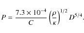
Here C, defined by Eq. (5.10) in Holsapple (2007), is a unitless parameter depending on the asteroid shape (approximated by a triaxial ellipsoid) and the angle of friction, $\rho$ is the asteroid bulk density, $\kappa$ is the tensile strength coefficient, and D is the effective diameter in meters.

Is is assumed (Holsapple 2007) that the tensile strength k of asteroids is size-dependent. The actual relation between k and D is related to the distribution of cracks throughout the body. Housen & Holsapple (1999) showed, that for a wide range of samples, $k=\kappa r^{-1/2}$ , where r=D/2. To estimate the value of $\kappa$ , one would have to apply static pressure to a sample of asteroid material. This has been done for various meteorite samples and terrestrial rocks, but the results may not be applicable to actual objects observed in space. Recently, the disintegration of 2008 TC₃ in the atmosphere presented a unique opportunity to estimate the dynamic loading at which fragmentation occurred (Jenniskens et al. 2009). It was assumed that this pressure is equal to the tensile strength of the body, although Nemtchinov & Popova (1997) suggest it should actually be 2.7 times greater.

$\begin{figure} \par\resizebox{9cm}{!}{\includegraphics[clip]{13468f16.eps}} \end{figure}$	Figure 16: Plot of the asteroid rotation periods P versus their effective diameters D. The sloped lines are maximum spin limits, drawn for the strength coefficients $\kappa= 10^{5}~{\rm N}~{\rm m}^{-3/2}$ , $\kappa= 10^{6}~{\rm N}~{\rm m}^{-3/2}$ , and densities $\rho=2500~{\rm kg}~{\rm m}^{-3}$ , $\rho=5000~{\rm kg}~{\rm m}^{-3}$ .
Open with DEXTER

Similar estimates were made for a number of fireballs. Selected results, for the largest of them, are presented in Table 4. As bolide fragmentation is often a multi-stage process, we compute two values for the strength coefficient: the minimal $\kappa$ for the first breake-up and the average $\kappa$ for the main body disruption. For simplicity we assume the atmospheric load at the time of fragmentation is the same as the tensile strength of the body k and consider it to contain fully cracked material. The Carancas meteorite, considered to be a monolithic body with few cracks, is an exception here as it survived atmospheric entry without fragmentation. For comparison we also quote the results obtained by Housen & Holsapple (1999) for granite specimens.

Table 4: Tensile strengths of selected stony fireballs.

Based on the values of $\kappa$ from Table 4, we assume for the asteroid material a minimum value $\kappa \sim 10^5~{\rm N}~{\rm m}^{-3/2}$ for the tensile strength coefficient.

To compute the spin limits for our sample of VSAs we assume, for an average asteroid, a moderately elongated shape of prolate ellipsoid (with b/a=0.7, c/a=0.7), a typical angle of friction of $\phi=40\hbox{$^\circ$ }$ (Richardson et al. 2005), a density of $\rho=2500~{\rm kg}~{\rm m}^{-3}$ , and the strength coefficient $\kappa= 10^{5}~{\rm N}~{\rm m}^{-3/2}$ ( $10^{7}~{\rm dynes}~ {\rm cm}^{-3/2}$ ). The line obtained with these parameters is shown in Fig. 16. While its slope depends on the exponent of D, the actual position is most sensitive to $\kappa$ and $\rho$ . To show this we replotted the line for two other combinations of $\kappa$ and $\rho$ .

A comparison of the limit spins in Fig. 16 with the observed rotation periods shows that the line obtained with $\kappa= 10^{5}~{\rm N}~{\rm m}^{-3/2}$ and a typical asteroid density is a reasonable match to the present data with only one object displaced significantly to the right of it (2000 WH₁₀). It is thus possible, that this line indeed marks the approximate border at which most asteroids undergo fragmentation due to the centrifugal forces. However, its significance needs to be confirmed with more data, which are not easy to collect. We note that a similar border was first proposed by Holsapple (2007), but he did not present justification for his choice of the tensile strength coefficient $\kappa=2.25\times 10^{5}~{\rm N}~ {\rm m}^{-3/2}$ .

In Fig. 16 there is a gap between the spin limit line and the majority of asteroids which seem to form another border of slightly greater slope and smaller $\kappa$ . This could be the effect of observational biases, uncertainties in the effective diameters, differences in the asteroid taxonomy types and/or the approximate nature of the theory predicting the tensile strength of these bodies. However, there is still one more possibility which we want to consider.

Figure 16 presents a snapshot of the continuous evolution of rotation periods of asteroids, mainly due to the YORP effect. In Paper II we discussed briefly the influence of YORP on the rotation of VSAs and mentioned near-Earth asteroids, for which this effect was observed. Among VSAs there is only one object - (54509) 2000 PH₅ - for which the YORP effect has been detected. Lowry et al. (2007) performed a simulation that numerically propagated the orbits of 2000 PH₅ and its 999 close clones into the future and followed the evolution of their spin states. They found that after about 5 Myr 75% of particles survived, and that their median rotation period was about 90 s. After 15 Myr 50% of clones survived with a median period of about 40 s.

In Fig. 16 we mark the spin evolution of 2000 PH₅ with a vertical arrow, which begins at its current spin of P=0.2029 h and ends at P=0.01 h, where the asteroid has a 50% probability of moving to after 15 Myr. After 5 Myr, 2000 PH₅ should cross the continuous line marking the spin limit, where its period will be about P=0.025 h.

While we do not have similar evolutionary tracks computed for other VSAs, the example of 2000 PH₅ shows us that the time taken to increase the rotation rate towards the spin limit can be comparable to the dynamical life-time of a typical near-Earth asteroid (which, according to Gladman et al. 2000, has a median value of about 10 Myr). What is more, the intensity of the YORP effect is inversely proportional to the diameter squared, so that objects larger than 2000 PH₅ will, on average, need more time to reach the spin limit line. Many of them may never do it before they are removed from the population of NEAs. This effect could explain the gap (which increases with diameter) in Fig. 16 between the spin limit line and the majority of VSAs.

Of course, the time taken to reach the spin limit line depends also on the initial period with which the asteroid enters the population of NEAs. While the intensity of the YORP effect in the Main Belt is about an order of magnitude smaller than in theEarth's neighborhood, the dynamical life-time is much longer. This leaves a lot of time for some of the Main-Belt VSAs, after their creation during collisions of larger bodies, to increase their spins prior to transferring to a near-Earth orbit. This effect of increasing the rotation rate due to the YORP effect is visible, for example, in histograms obtained for small MBAs of different diameters by Warner et al. (2009). Recently Masiero et al. (2009) observed many small MBAs and also found a deviation from the Maxwellian distribution both for the slow and fast rotating objects. These studies, however, included asteroids of diameters generally greater than 1 km. In the case of VSAs, this deviation from the collision-shaped Maxwellian distribution can be much larger and the number of fast rotation asteroids greater. Clearly, these issues await a more thorough investigation.

4 Conclusions and future work

This is the final paper in a series of three, summarizing results of a survey of very small, near-Earth asteroids using the SALT telescope. In total, we have obtained new periods for 26 very small asteroids on near-Earth orbits, which increases the number of known spins by about 50%. One of the asteroids was found to be a possible non-principal axis (NPA) rotator, which adds to the 3 previously known NPA rotation asteroids.

The analysis of spin limits shows that the tensile strength of VSAs, after scaling them to the same size, is of the same order as the minimum tensile strength estimated for stony meteoroids undergoing fragmentation in the atmosphere. This result is tentative and needs confirmation with more data. There is a lack of larger VSAs close to the spin limit which may be caused by selection effects or other reasons. To investigate this issue we have started a new survey of small NEAs with SALT, paying more attention to the asteroids in the 20 < H < 21.5 mag region. The data are already collected and we are now in the process of analyzing them. Results will be published in a following paper.

Acknowledgements

TK is grateful to A. Kryszczynska, and E. Bruss-Kwiatkowska for their help in reduction of some of data. An anonymous referee made helpful comments which improved the paper. MP was supported by the Polish MNiSW grant N N203 387937. All of the observations reported in this paper were obtained with the Southern African Large Telescope (SALT).

References

Birtwhistle, P. 2009, Minor Planet Bulletin, 36, 186 [NASA ADS] [Google Scholar]
Borovicka, J., & Spurný, P. 2008, A&A, 485, L1 [NASA ADS] [CrossRef] [EDP Sciences] [Google Scholar]
Gladman, B., Michel, P., & Froeschlé, C. 2000, Icarus, 146, 176 [NASA ADS] [CrossRef] [Google Scholar]
Holsapple, K. A. 2007, Icarus, 187, 500 [NASA ADS] [CrossRef] [Google Scholar]
Housen, K. R., & Holsapple, K. A. 1999, Icarus, 142, 21 [NASA ADS] [CrossRef] [Google Scholar]
Hudson, R. S., & Ostro, S. J. 1995, Science, 270, 84 [NASA ADS] [CrossRef] [Google Scholar]
Hudson, R. S., & Ostro, S. J. 1999, Icarus, 140, 369 [NASA ADS] [CrossRef] [Google Scholar]
Jenniskens, P., Shaddad, M. H., Numan, D., et al. 2009, Nature, 458, 485 [NASA ADS] [CrossRef] [PubMed] [Google Scholar]
Kwiatkowski, T. 2010, A&A, 509, A95 [NASA ADS] [CrossRef] [EDP Sciences] [Google Scholar]
Kwiatkowski, T., Kryszczynska, A., Polinska, M., et al. 2009, A&A, 495, 967 [NASA ADS] [CrossRef] [EDP Sciences] [Google Scholar]
Kwiatkowski, T., Buckley, D. A. H., O'Donoghue, D., et al. 2010, A&A, 509, A94 [NASA ADS] [CrossRef] [EDP Sciences] [Google Scholar]
Lowry, S. C., Fitzsimmons, A., Pravec, P., et al. 2007, Science, 316, 272 [NASA ADS] [CrossRef] [PubMed] [Google Scholar]
Mann, R. K., Jewitt, D., & Lacerda, P. 2007, AJ, 134, 1133 [NASA ADS] [CrossRef] [Google Scholar]
Masiero, J., Jedicke, R., Durech, J., et al. 2009, Icarus, 145 [NASA ADS] [CrossRef] [Google Scholar]
Nemtchinov, I. V., & Popova, O. P. 1997, Solar System Research, 31, 408 [NASA ADS] [Google Scholar]
Pravec, P., & Harris, A. W. 2000, Icarus, 148, 12 [NASA ADS] [CrossRef] [Google Scholar]
Pravec, P., Harris, A. W., Vokrouhlicky, D., et al. 2008, Icarus, 197, 497 [NASA ADS] [CrossRef] [Google Scholar]
Richardson, D. C., Elankumaran, P., & Sanderson, R. E. 2005, Icarus, 173, 349 [NASA ADS] [CrossRef] [Google Scholar]
Warner, B. D., Harris, A. W., & Pravec, P. 2009, Icarus, 202, 134 [NASA ADS] [CrossRef] [Google Scholar]
Whiteley, R. J., Hergenrother, C. W., & Tholen, D. J. 2002a, in Proceedings of Asteroids, Comets, Meteors 2002, ed. B. Warmbein (Noordwijk, Netherlands), ESA SP-500, 473 [Google Scholar]
Whiteley, R. J., Tholen, D. J., & Hergenrother, C. W. 2002b, Icarus, 157, 139 [NASA ADS] [CrossRef] [Google Scholar]

Footnotes

... telescope: Based on observations made with the Southern African Large Telescope (SALT).
...: Photometric data are only available in electronic form at the CDS via anonymous ftp to cdsarc.u-strasbg.fr (130.79.128.5) or via http://cdsweb.u-strasbg.fr/cgi-bin/qcat?J/A+A/511/A49
... Base: http://www.minorplanetobserver.com/astlc/LightcurveParameters.htm

All Tables

Table 1: Aspect data and the observing log.

Table 2: Summary of the results.

Table 3: Negative detections.

Table 4: Tensile strengths of selected stony fireballs.

All Figures

$\begin{figure} \par\resizebox{9cm}{!}{\includegraphics[clip]{13468f01.eps}} \end{figure}$	Figure 1: Composite lightcurve of 2007 CX₅₀ obtained with a period P=1.45 h. The part of the Fourier fit beyond the 0.65 phase is unconstrained by the data and serves only as an example. The zero phase in this and the subsequent plots is corrected for light-time.
Open with DEXTER
In the text

$\begin{figure} \par\resizebox{9cm}{!}{\includegraphics[clip]{13468f02.eps}} \end{figure}$	Figure 2: $\chi ^2$ plot for 2007 EO.
Open with DEXTER
In the text

$\begin{figure} \par\resizebox{9cm}{!}{\includegraphics[clip]{13468f03.eps}} \end{figure}$	Figure 3: Composite lightcurves obtained for 2007 EO with two periods: P₁'=2.76 h and P₂'=2.25 h, both of which are acceptable.
Open with DEXTER
In the text

$\begin{figure} \par\resizebox{9cm}{!}{\includegraphics[clip]{13468f04.eps}} \end{figure}$	Figure 4: Composite lightcurve of 2007 GU1 obtained with a period P=4.1 h. It is given only to show the available data. The true lightcurve can have quite different shape than the fitted Fourier series.
Open with DEXTER
In the text

$\begin{figure} \par\resizebox{9cm}{!}{\includegraphics[clip]{13468f05.eps}} \end{figure}$	Figure 5: Composite lightcurve of 2007 HL4. Period $P=1.48 \pm 0.02$ h.
Open with DEXTER
In the text

$\begin{figure} \par\resizebox{9cm}{!}{\includegraphics[clip]{13468f06.eps}} \par\end{figure}$	Figure 6: Composite lightcurve of 2007 RE2 obtained with a period P=0.995 h. It is not a unique solution and is given only to show the available data. The accepted period of 2007 RE₂ is $1 \pm 0.2$ h.
Open with DEXTER
In the text

$\begin{figure} \par\resizebox{9cm}{!}{\includegraphics[clip]{13468f07.eps}} \end{figure}$	Figure 7: Composite lightcurve of 2007 UC₂ obtained with the period P=0.527 h.
Open with DEXTER
In the text

$\begin{figure} \par\resizebox{9cm}{!}{\includegraphics[clip]{13468f08.eps}} \end{figure}$	Figure 8: Composite lightcurve of 2007 RY₉ obtained with the period P=1.2 h.
Open with DEXTER
In the text

$\begin{figure} \par\resizebox{9cm}{!}{\includegraphics[clip]{13468f09.eps}} \end{figure}$	Figure 9: Lightcurve of 2007 TS₂₄.
Open with DEXTER
In the text

$\begin{figure} \par\resizebox{9cm}{!}{\includegraphics[clip]{13468f10.eps}} \end{figure}$	Figure 10: Example composite lightcurve of 2007 UG6 obtained with P=1.85 h, while the formal solution for the period is $P=1.82 \pm 0.07$ h.
Open with DEXTER
In the text

$\begin{figure} \par\resizebox{9cm}{!}{\includegraphics[clip]{13468f11.eps}} \end{figure}$	Figure 11: Lightcurves of 2007 XN₁₆ showing signs of non-principal axis rotation.
Open with DEXTER
In the text

$\begin{figure} \par\resizebox{9cm}{!}{\includegraphics[clip]{13468f12.eps}} \end{figure}$	Figure 12: Composite lightcurve of 2007 XN₁₆ obtained with a period of P=1.835 h.
Open with DEXTER
In the text

$\begin{figure} \par\resizebox{9cm}{!}{\includegraphics[clip]{13468f13.eps}} \par\end{figure}$	Figure 13: Composite lightcurve of 2008 CP₁₁₆ obtained with the period P=0.327 h using the 29 Feb. data. The accepted solution (derived from both 28 and 29 Feb.) for this asteroid is P=0.330 h.
Open with DEXTER
In the text

$\begin{figure} \par\resizebox{9cm}{!}{\includegraphics[clip]{13468f14.eps}} \end{figure}$	Figure 14: Peculiar lightcurves of 2007 RQ₁₂. Both the upper and the lower panels are drawn to the same scale. The second part of the East track data (marked by squares) is arbitrarily shifted in magnitude.
Open with DEXTER
In the text

$\begin{figure} \par\resizebox{9cm}{!}{\includegraphics[clip]{13468f15.eps}} \end{figure}$	Figure 15: Histogram of spin rates of VSAs. In order to shorten the abscissa, we have omitted 2008 HJ, which has the spin rate of $f=84.4~ {\rm h}^{-1}$ . The inset plot displays in more detail the left part of the original histogram, where most objects are located.
Open with DEXTER
In the text

$\begin{figure} \par\resizebox{9cm}{!}{\includegraphics[clip]{13468f16.eps}} \end{figure}$	Figure 16: Plot of the asteroid rotation periods P versus their effective diameters D. The sloped lines are maximum spin limits, drawn for the strength coefficients $\kappa= 10^{5}~{\rm N}~{\rm m}^{-3/2}$ , $\kappa= 10^{6}~{\rm N}~{\rm m}^{-3/2}$ , and densities $\rho=2500~{\rm kg}~{\rm m}^{-3}$ , $\rho=5000~{\rm kg}~{\rm m}^{-3}$ .
Open with DEXTER
In the text

Current usage metrics show cumulative count of Article Views (full-text article views including HTML views, PDF and ePub downloads, according to the available data) and Abstracts Views on Vision4Press platform.

Data correspond to usage on the plateform after 2015. The current usage metrics is available 48-96 hours after online publication and is updated daily on week days.

Initial download of the metrics may take a while.

[1] Birtwhistle, P. 2009, Minor Planet Bulletin, 36, 186 [NASA ADS] [Google Scholar]

[2] Borovicka, J., & Spurný, P. 2008, A&A, 485, L1 [NASA ADS] [CrossRef] [EDP Sciences] [Google Scholar]

[3] Gladman, B., Michel, P., & Froeschlé, C. 2000, Icarus, 146, 176 [NASA ADS] [CrossRef] [Google Scholar]

[4] Holsapple, K. A. 2007, Icarus, 187, 500 [NASA ADS] [CrossRef] [Google Scholar]

[5] Housen, K. R., & Holsapple, K. A. 1999, Icarus, 142, 21 [NASA ADS] [CrossRef] [Google Scholar]

[6] Hudson, R. S., & Ostro, S. J. 1995, Science, 270, 84 [NASA ADS] [CrossRef] [Google Scholar]

[7] Hudson, R. S., & Ostro, S. J. 1999, Icarus, 140, 369 [NASA ADS] [CrossRef] [Google Scholar]

[8] Jenniskens, P., Shaddad, M. H., Numan, D., et al. 2009, Nature, 458, 485 [NASA ADS] [CrossRef] [PubMed] [Google Scholar]

[9] Kwiatkowski, T. 2010, A&A, 509, A95 [NASA ADS] [CrossRef] [EDP Sciences] [Google Scholar]

[10] Kwiatkowski, T., Kryszczynska, A., Polinska, M., et al. 2009, A&A, 495, 967 [NASA ADS] [CrossRef] [EDP Sciences] [Google Scholar]

[11] Kwiatkowski, T., Buckley, D. A. H., O'Donoghue, D., et al. 2010, A&A, 509, A94 [NASA ADS] [CrossRef] [EDP Sciences] [Google Scholar]

[12] Lowry, S. C., Fitzsimmons, A., Pravec, P., et al. 2007, Science, 316, 272 [NASA ADS] [CrossRef] [PubMed] [Google Scholar]

[13] Mann, R. K., Jewitt, D., & Lacerda, P. 2007, AJ, 134, 1133 [NASA ADS] [CrossRef] [Google Scholar]

[14] Masiero, J., Jedicke, R., Durech, J., et al. 2009, Icarus, 145 [NASA ADS] [CrossRef] [Google Scholar]

[15] Nemtchinov, I. V., & Popova, O. P. 1997, Solar System Research, 31, 408 [NASA ADS] [Google Scholar]

[16] Pravec, P., & Harris, A. W. 2000, Icarus, 148, 12 [NASA ADS] [CrossRef] [Google Scholar]

[17] Pravec, P., Harris, A. W., Vokrouhlicky, D., et al. 2008, Icarus, 197, 497 [NASA ADS] [CrossRef] [Google Scholar]

[18] Richardson, D. C., Elankumaran, P., & Sanderson, R. E. 2005, Icarus, 173, 349 [NASA ADS] [CrossRef] [Google Scholar]

[19] Warner, B. D., Harris, A. W., & Pravec, P. 2009, Icarus, 202, 134 [NASA ADS] [CrossRef] [Google Scholar]

[20] Whiteley, R. J., Hergenrother, C. W., & Tholen, D. J. 2002a, in Proceedings of Asteroids, Comets, Meteors 2002, ed. B. Warmbein (Noordwijk, Netherlands), ESA SP-500, 473 [Google Scholar]

[21] Whiteley, R. J., Tholen, D. J., & Hergenrother, C. W. 2002b, Icarus, 157, 139 [NASA ADS] [CrossRef] [Google Scholar]

Photometric survey of the very small near-Earth asteroids with the SALT telescope,

III. Lightcurves and periods for 12 objects and negative detections

1 Introduction

2 Lightcurves of 12 asteroids

2.1 2007 CX50

2.2 2007 EO

2.3 2007 GU1

2.4 2007 HL4

2.5 2007 RE2

2.6 2007 UC2

2.7 2007 RY9

2.8 2007 TS24

2.9 2007 UG6

2.10 2007 XN16

2.11 2008 CP116

2.12 2007 RQ12